Dissertations 2018
Evaluation of traffic speed control devices and its
applications
Shefang Wang
Iowa State University
Follow this and additional works at:https://lib.dr.iastate.edu/etd Part of theCivil Engineering Commons
This Dissertation is brought to you for free and open access by the Iowa State University Capstones, Theses and Dissertations at Iowa State University Digital Repository. It has been accepted for inclusion in Graduate Theses and Dissertations by an authorized administrator of Iowa State University Digital Repository. For more information, please [email protected].
Recommended Citation
Wang, Shefang, "Evaluation of traffic speed control devices and its applications" (2018).Graduate Theses and Dissertations. 16689.
Evaluation of traffic speed control devices and its applications
by
Shefang Wang
A dissertation submitted to the graduate faculty in partial fulfillment of the requirements for the degree of
DOCTOR OF PHILOSOPHY
Major: Civil Engineering (Transportation Engineering)
Program of Study Committee: Anuj Sharma, Major Professor
Jing Dong Peter Savolainen Alicia Carriquiry Soumik Sarkar
The student author, whose presentation of the scholarship herein was approved by the program of study committee, is solely responsible for the content of this dissertation. The
Graduate College will ensure this dissertation is globally accessible and will not permit alterations after a degree is conferred.
Iowa State University Ames, Iowa
2018
TABLE OF CONTENTS Page LIST OF FIGURES ... iv LIST OF TABLES ... vi NOMENCLATURE ... vii ABSTRACT ... ix CHAPTER 1. INTRODUCTION ... 1
1.1 Static Traffic Speed Control Device — Speed Limit Sign ... 1
1.1.1 Safety Study of Speed-Limit Reduction ... 2
1.1.2 Empirical Study of Speed-Limit Reduction ... 3
1.2 Dynamic Traffic Speed Control Devices — Changeable Message Sign ... 4
1.2.1 Variable Speed Limit ... 4
1.2.2 Variable Speed Limit in Work Zone ... 5
1.2.3 Variable Speed Limit in Inclement Weather ... 6
1.3 Summary ... 7
1.4 Dissertation Structure ... 7
CHAPTER 2. PROBLEM STATEMENT ... 9
2.1 Dynamic Message Sign in Work Zone ... 10
2.2 Variable Advisory Speed Limit Sign in Severe Weather ... 14
2.3 Problem Statement ... 15
2.3.1 Data Smoothing ... 15
2.3.2 Labels for Changeable Messages ... 17
2.4 Summary ... 19
CHAPTER 3. APPLICATIONS ... 20
3.1 Introduction to Application Pipeline ... 20
3.1.1 Data Processing Module ... 20
3.1.2 Historical Data Analysis Module ... 21
3.2.1 DMS in I-74 Bridge Repair Work Zone ... 23
3.2.2 Variable Advisory Speed Limit in Snow Events ... 25
3.2.2.1 Real-time implementation & validation example #1 ... 27
3.2.2.2 Real-time implementation & validation example #2 ... 30
3.2.3 Text Alert in Iowa Work Zones ... 32
3.3 Extension Applications of the Current Research ... 35
3.3.1 Traffic Management Center Data Feed API ... 35
3.3.2 Work Zone Performance Evaluation ... 36
3.4 Summary ... 38
CHAPTER 4. OLDER DRIVERS NATURALISTIC DRIVING STUDY ... 40
4.1 Introduction ... 40
4.2 Data Sources ... 42
4.2.1 Instrumented Vehicle Sensors... 43
4.2.2 Nebraska Geographic Information System Database ... 45
4.2.3 Driver’s Information ... 45 4.3 Data Pre-Processing ... 47 4.4 Descriptive Statistics ... 51 4.4.1 Driver’s Information ... 51 4.4.2 Modeling Dataset ... 54 4.5 Statistical Method ... 59 4.6 Modeling Results... 60
4.6.1 Mixed-effect Linear Regression ... 60
4.6.2 Mixed-effect Multinomial Logistic Regression ... 64
4.7 Discussion ... 67 4.8 Summary ... 69 CHAPTER 5. CONCLUSIONS ... 70 5.1 Research Highlight ... 70 5.2 Future Research ... 71 REFERENCES ... 73
LIST OF FIGURES
Page
Figure 2.1 DMS Study Area (Google Maps, 2017) ... 11
Figure 2.2 Existing DMS Performance ... 12
Figure 2.3 DMS Displayed Messages, Sensor Speed, and Occupancy ... 13
Figure 2.4 Performance of Existing Control Logic ... 15
Figure 2.5 Data Smoothing ... 17
Figure 3.1 Application Pipeline ... 21
Figure 3.2 Labels and Decision Boundaries for DMS in Work Zone ... 23
Figure 3.3 Existing Logic and Proposed DMS Control Logic... 24
Figure 3.4 Existing Logic and Proposed Control Logic ... 26
Figure 3.5 Event #1 Speed Profile and Roadway Surface Condition ... 28
Figure 3.6 Event #1 TransSuite TIS Software Report ... 28
Figure 3.7 Event #1 Roadway Surface Conditions ... 29
Figure 3.8 Event #2 Speed Profile and Roadway Surface Condition ... 30
Figure 3.9 Event #2 Camera View of Roadway Conditions ... 31
Figure 3.10 Event # 2 TransSuite TIS Software Report ... 31
Figure 3.11 Camera View of the Traffic Event on December 27, 2017 ... 32
Figure 3.12 Example of Text Alert Application ... 33
Figure 3.13 Example of Text Alert Application with Multiple Sensors ... 34
Figure 3.14 Operations Dashboard with Work Zone Alert Feed ... 36
Figure 3.15 2017 Iowa Work Zone Map ... 37
Figure 4.1 Image for Accelerometer Data Collected by IMU ... 43
Figure 4.2 Driving Routes Visualization of UNMC Old Driver Study ... 44
Figure 4.3 GIS Polyline Shapefile of Nebraska ... 45
Figure 4.4 Undesired Trips Example — Making Right Turn at an Intersection ... 48
Figure 4.5 Undesired Trips Example — Traffic Accident ... 49
Figure 4.6 Data Filtering Examples ... 50
Figure 4.7 Data Pre-Processing Flow Chart ... 51
Figure 4.8 Parallel Coordinate Plot of Driver Information ... 53
Figure 4.9 Pair Wised Scatter Plot of Driver Information ... 54
LIST OF TABLES
Page
Table 3.1 Performance Comparisons between Proposed and Existing Logic ... 26
Table 4.1 Summary of Statistics for Drivers ... 52
Table 4.2 Summary of Statistics for Categorical Variables ... 58
Table 4.3 Summary of Statistics for Continuous Variables ... 59
Table 4.4 Mixed Effect Linear Regression ... 61
Table 4.5 Mixed Effect Multinomial Logistic Regression — Slowing ... 64
NOMENCLATURE
AADT Annual Average Daily Traffic API Application Programming Interface ATMS Advanced Traffic Management System
AWF Advance Warning Flasher
CMS Changeable Message Signs
DMS Dynamic Message Sign
DOM Document Object Model
DOT Department of Transportation GIS Geographic Information System
GPS Global Positioning System
HSSI High Speed Signalized Intersection IMU Inertial Measurement Unit
InTrans Institute for Transportation at Iowa State University NDS Naturalistic Driving Study
OBD On-Board Diagnostics
REACTOR Lab Real-time Analytics of Transportation Data lab SHRP 2 Second Strategic Highway Research Program
TMC Traffic Management Center
UFOV Useful Filed of View
UNMC University of Nebraska Medical Center
VTTI Virginia Tech Transportation Institute
XML Extensible Markup Language
ABSTRACT
Traffic speed control devices have an important role in transportation systems. Static devices, such as speed limit signs, can advocate safe and efficient traffic movements by displaying appropriate speed limits. Changeable message signs have many applications in adjusting the dynamic nature of a transportation system. These applications include but are not limited to variable speed limits based on ambient traffic conditions, work zone
management, and warnings about severe weather conditions.
This dissertation evaluated the performance of multiple traffic speed control devices, including static speed limit signs and dynamic changeable message signs. By identifying existing problems, such as data smoothing, traffic characteristics clustering, and event classification, the author proposed some practical engineering solutions for better
performance. One of the highlighted applications is a text alert system that actively monitors 50 Iowa work zones, which are equipped with more than 350 roadway sensors, and sends multimedia alert texts to district traffic engineers. The application of a variable advisory speed limit system that reports severe winter weather conditions was also
implemented/validated and currently runs in “ghost” mode (without displaying any visible messages to the public) until it is approved.
After conducting a series of analyses in the transportation macroscopic world (data collected by roadway traffic sensors), the current dissertation research expanded into the microscopic driver speed behavior analysis (data collected by instrumented vehicle sensors). A naturalistic driving study focusing on older drivers collected a large amount of detailed individual driving data from multiple sources with high resolutions, including timestamped
speed, acceleration, deceleration, and geo locations. This abundant dataset enabled the author to examine an individual’s driving behavior with respect to different speed limits and other factors.
CHAPTER 1. INTRODUCTION
Traffic speed control devices have an important role in modern transportation systems. Static devices such as speed limit signs inform drivers about the appropriate speed limit along a certain roadway segment. Devices such as changeable message signs, which are extensively employed, can better adapt to the dynamic nature of a transportation system. In this chapter, a literature review is conducted to address static and dynamic traffic speed control devices.
1.1 Static Traffic Speed Control Device — Speed Limit Sign
A roadway network is extensively equipped with speed limit signs, which are located at the points where the posted speed limit changes. When establishing a speed limit within a speed zone, an engineering study should be conducted, and the posted speed limit should be within 5 mph of the 85th percentile free-flow traffic speed. Speed limits are used to enhance road safety, which can be achieved by either a limiting function or a coordinating function (TRB Committee for Guidance on Setting and Enforcing Speed Limits, 1998). A limiting function establishes a maximum speed limit along roads, which can reduce the likelihood and severity of a crash. A coordinating function reduces the speed variance along roads, which produces a more uniform traffic flow.
With regard to speed limit reductions, many studies have demonstrated that lower speeds and speed variances can reduce the severity and frequency of crashes (Liu & Popoff, 1997)(Aarts & van Schagen, 2006)(Elvik et al., 2004)(Hamzeie et al., 2017). Several strategies, such as variable speed limit control (van den Hoogen & Smulders, 1994), dynamic speed display signs
(Ullman & Rose, 2005), speed transition zones (Cruzado & Donnell, 2010a), rational speed limits (Son et al., 2009), and dynamic curve warning systems (Monsere et al., 2005), have been assessed for their effectiveness in reducing the speeds and speed variability of approaching vehicles. These studies confirm that arbitrary changes in speed limits have a limited impact on drivers’ speed choices and may even lower drivers’ compliance with the posted speed limits. Lower driver compliance can potentially increase the speed variance, which creates unsafe conditions. Another important trend that was observed in the previously mentioned studies is that the actual reduction in driver speed is often lower than the actual reduction in speed limit. The extent of this reduction in driver speed can vary depending on the reason for the application.
1.1.1 Safety Study of Speed-Limit Reduction
In a recent study of 56 high-speed approaches at high-speed signalized intersections (HSSIs) in Nebraska, Wu et al. (2013) reported that the effect of a 5 mph speed limit reduction in conjunction with advance warning flashers (AWFs) was ambiguous because it reduced the frequency of crashes on some intersection approaches but increased the frequency of crashes on others. Conversely, a 10 mph reduction in speed limit with AWF unambiguously decreased both the accident frequency and the injury severity of crashes. In the presence of potentially
heterogeneous driver responses to decreased speed limits, this study speculated that reductions in variability and actual speeds due to a 5 mph reduction in speed limit was not always sufficient for unambiguously decreasing the frequency and severity of crashes. However, reductions in variability and actual speed were sufficient for unambiguously decreasing the frequency and severity of crashes when the speed limit reduction was 10 mph. This crash study stresses the
need for an empirical study investigating the impact of different ranges of speed limit reductions on drivers’ speed choices at an HSSI.
1.1.2 Empirical Study of Speed-Limit Reduction
Wang et al. (2017) extended the research on HSSIs (Wu et al., 2013) and conducted an empirical study to investigate the scenario in which the speed limit is reduced near the stop line at intersections by a permanent posted speed limit sign. Different speed limit reduction scenarios were assessed by analyzing the empirical speed distribution of vehicles as they approached an HSSI equipped with AWFs. The study sites consisted of six approaches: two approaches without any speed limit reductions, two approaches with a 5 mph reduction (from 60 mph to 55 mph), and two approaches with a 10 mph reduction (from 65 mph to 55 mph). For each high-speed intersection approach, vehicle speed trajectory data were collected at two locations. The first location was near a speed limit sign and ranged from approximately 1,000 to 2,000 ft from the intersection stop line. The second location was a downstream data collection point approximately 500 ft from the intersection.
After data cleaning and validation, 12,401 free-flow vehicle trajectories were obtained. The constant speed limit group had 4,289 observations; the 5 mph speed limit group had 5,503 observations; and 2,609 trajectories were observed in the 10 mph reduction group. Six speed models were separately constructed for each signalized intersection approach. Within each model, seven quantiles were reported using quantile regression: 10th, 15th, 25th, 50th, 75th, 85th, and 90th. In this empirical speed limit study, the drivers’ observed average speeds hovered in the range of 1.1–2.5 mph higher than the regulatory speed limit, which is possibly a comfortable speed range, near a signalized intersection. For sites without any speed limit reductions and a 5
mph reduction, a speed-limit compliance rate of 30–40% was observed at the near-stop-line location. For sites with a 10 mph reduction, a speed limit compliance rate of 40–50% was observed at the near-stop-line location. In addition, this study provides another example that the ambient condition, rather than speed enforcement, has an important role in drivers’ speed
choices. If driver behavior were significantly affected by the regulatory speed limit, then the rate of compliance rate with the speed limit would tend to be a constant number.
1.2 Dynamic Traffic Speed Control Devices — Changeable Message Sign
Changeable message signs (CMSs), also known as “dynamic message signs” or “variable message signs”, have been installed on U.S. roadways since the 1960s. These signs aim to reduce traffic delay, accident risk, or special roadway conditions; postpone or prevent congestion; and harmonize traffic flows during peak periods (Bertini et al., 2006)(Mounce et al., 2006). A dynamic message may be triggered by an operator in a traffic management center by sensor inputs installed in the roadway network or prescheduled message plans. By dynamically adapting to complex traffic conditions, these systems can improve lane utilization and provide a calmer driving experience due to the measured reductions in crash frequency and severity (Allaby et al., 2007).
1.2.1 Variable Speed Limit
Highway agencies spend millions of dollars in an effort to ensure safe and efficient travel. Regardless of maintenance investment and activities, other factors, particularly driver behavior during non-recurring events (inclement weather or traffic incidents), can significantly impact safety. A variable speed limit (VSL) system, which is triggered by atmospheric, surface,
and/or traffic conditions is a commonly deployed safety countermeasure for warning drivers about imminent risks and suggesting an appropriate speed for existing conditions.
Bertini et al. (2006) collected lane-based one-minute loop data on a German autobahn and extracted information about the speed, count, and density between sensors for their VSL logic. Their analysis illustrated a strong correlation between the displayed speed limit and the real traffic dynamics and indicated that a reduced speed limit prior to a bottleneck could manage dense traffic. Abdel-Aty et al. (2006) investigated the safety effects of VSLs based on
PARAMICS micro-simulation. In their study, the target area was a 36-mile corridor of Interstate-4 around the Orlando metropolitan area, and the collected data included average vehicle counts, speed, and occupancy collected via loops. Based on the crash likelihood observed in real time, the authors provided several recommendations for VSL implementation: gradually changing the speed limit over time and abruptly in space, reducing the upstream speed limit while increasing the downstream speed limit, and so on. Instead of collecting data from point detector, Kattan et al. (2015) presented a VSL control algorithm based on the space mean speeds collected from probe vehicles. Their VSL logic was tested using the PARAMICS micro-simulation model and demonstrated improved traffic safety conditions.
1.2.2 Variable Speed Limit in Work Zone
Many researchers have explored the effect and logic of VSLs in work zones. Lin et al. (2004) explored the effectiveness of VSL signs on highway work zone operations. They proposed two online VSL algorithms to minimize the queues in advance of a work zone and maximize the throughput in a work zone area. Different CORSIM simulation models were run based on several lane closure configurations with control intervals set to 1 min, 5 min, 10 min,
and other intervals. Kang et al. (2004) conducted a similar study using CORSIM-RTE. Their online VSL algorithm aimed to maximize the total throughput based on the upstream volume, driver compliance rate, and congestion status. The product yielded a lower speed variance and delay, and higher throughput and speed along the work zone. In another VSL work zone
application (Allaby et al., 2007), the control logic varied every minute in 5-mph intervals, using 90-second measurements of lane-by-lane speed and volume. Researchers calculated the
maximum speed difference within the work zone during peak hours as a measure of
effectiveness. The findings showed a 25–35% reduction in the maximum speed differences in the work-zone area during the 6:00 to 8:00 a.m. morning peak traffic period and a 7% increase in the total throughput volume.
1.2.3 Variable Speed Limit in Inclement Weather
In addition to the dynamic nature of work zones, inclement weather is another essential factor that contributes to the complexity of a transportation system. Drivers’ behavior during non-recurring weather events can significantly impact roadway safety.
Katz et al. (2012) provided several guidelines for the use of VSL systems in wet weather, including displaying changes for a minimum of one minute and establishing a minimum speed limit of 30 mph. The authors also reported several VSL projects related to weather and their control strategies, based on pavement conditions, weather conditions, and visibility. (Katz et al., 2012) (Goodwin, 2003). For example, the Alabama Department of Transportation (DOT) operates a seven-mile-long corridor with 24 VSL signs along I-10 in Mobile. Based on the visibility distance, the speed limits are changed from 35 mph to 65 mph in increments of 10 mph. The Washington State DOT has implemented several VSL systems in both urban area and
mountainous areas. In urban areas, the speed limit is changed based on speed and occupancy sensors, whereas the speed limits in mountainous areas are manually established based on weather information. Similar to Alabama, the VSLs in Washington change the speed limits from 35 mph to 65 mph in 10-mph increments, and the control strategy is based on the visibility distance, weather information (rain, heavy rain, fog, and snow), and different pavement conditions (dry, wet, and icy). In central Florida, Hassan et al. (2012) conducted a thorough survey to investigate driver behavior and preferences for VSL systems in adverse visibility conditions. Their modeling results indicated that combining a VSL system with extra changeable message signs is the optimum strategy for improving roadway safety during inclement weather.
1.3 Summary
In this chapter, a literature review was conducted to address topics of static and dynamic traffic speed control devices. For static devices such as speed limit signs, in addition to the previous researches, two case studies of speed limit reduction were introduced from the author’s published work. Then, dynamic speed control devices were discussed with regard to work zones and inclement weather. In the next chapter, two applications of dynamic traffic speed control devices in Iowa are discussed. One is the dynamic message sign in work zones, and the other is variable speed limit in response to severe winter snow storms.
1.4 Dissertation Structure
Chapter 1 discusses historical research on different types of traffic speed control devices. Chapter 2 evaluates the performance of the existing speed control devices in Iowa, including DMSs in work zones and variable advisory speed limit in inclement weather. However, their
performance was not desirable due to several issues. By addressing identified problems, Chapter 3 significantly enhances the discussion of the performance of DMSs and variable advisory speed limit and provides multiple practical traffic speed control applications.
In addition to speed patterns in the macroscopic world, which is the focus in the first three chapters, this dissertation research explores a new microscopic world of transportation. A naturalist driving study is presented in Chapter 4, in which the study evaluates the older
population’s driving behaviors as a function of speed limit and other related factors. At last, Chapter 5 summarizes the research highlights and proposes future research ideas.
CHAPTER 2. PROBLEM STATEMENT
The Iowa Department of Transportation (DOT) maintains more than 500 Wavetronix sensors across the state to collect traffic data (speed, occupancy, and timestamp), which can be accessed via XML feeds with a refresh rate of 20 seconds. To archive the sensor data 24/7, a series of programs were coded to automatically download and parse the XML feeds daily. In addition to the traffic sensor data, message data displayed on changeable message signs (CMS) are archived by Iowa DOT’s advanced traffic management system (ATMS) software. This ATMS software can extract historical message data, including message content and the start and end times of the displayed messages.
After discussion with the Iowa DOT personnel, this dissertation research used three criteria as performance measures for the CMS message control algorithm: the total number of messages, number of short-duration messages, and number of fluctuating clusters. Although the total number of messages may not reflect a complete picture of the real conditions, signs with a large number of messages suggest a potential detection fault and need additional attention. Messages with durations less than 75 seconds or short-duration messages were likely related to high sensor noise. If multiple messages were generated in quick succession within a short amount of time (five minutes), these groups of messages were treated as a fluctuating message cluster. A high volume of fluctuating message clusters at a certain site can be confusing for drivers and demonstrates the instability of the control logic.
In the following paragraphs, two existing applications that manage highway traffic speed in Iowa are examined: 1) a dynamic message sign (DMS) application in a work zone, and 2) a variable advisory speed limit system that reports severe winter weather. Both of the applications
collected data based on nearby Wavetronix sensors and were supposed to communicate with roadway drivers with reliable traffic information. However, their performance is less than desirable and suggests room for improvement.
2.1 Dynamic Message Sign in Work Zone
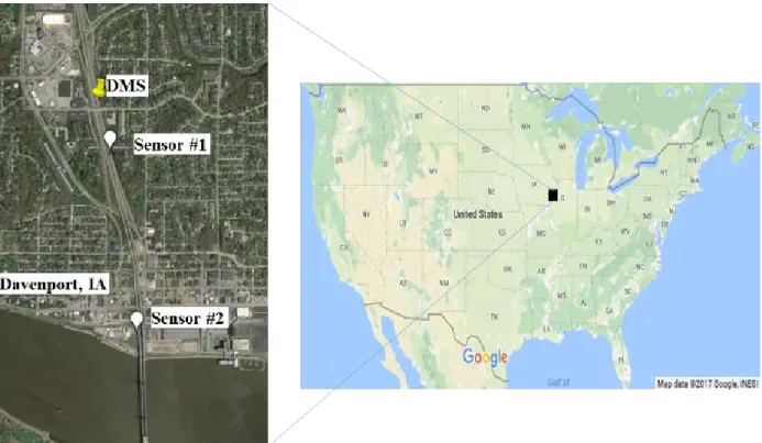
The study area was a two-mile work zone near Davenport, Iowa for the repair and
cleaning of an I-74 bridge (connects Iowa to Illinois). This highway facility has two lanes in each direction with a posted speed limit of 55 mph, and only one lane was permitted to be closed throughout the entire work area. A permanent side-mounted dynamic message sign was installed at the beginning of the work zone to provide traffic information for the southbound traffic. The existing message display logic is driven by two nearby Wavetronix sensors: the first sensor is 0.2 miles south of the DMS, and the second sensor is located one mile downstream. Based on
different levels of speed, the DMS displays one of three types of messages: “Traffic Delays Possible”, “Slow Traffic Ahead”, and “Stopped Traffic Ahead”. Figure 2.1 shows the study area, where the white drops represent two Wavetronix sensors and the yellow pin indicates the
location of the target DMS.
This task aimed to validate the existing DMS performance by using Sensor #2, which is located in the neighborhood of one mile downstream of the DMS, to detect the traffic conditions within the work zone. By synchronizing the sensor and DMS message data, the task tested whether displayed messages can provide realistic, reliable, and real-time traffic information.
Figure 2.1 DMS Study Area (Google Maps, 2017)
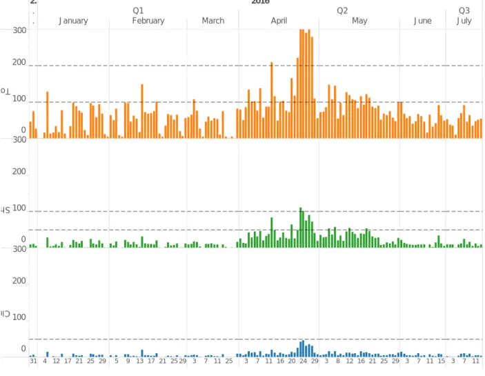
Figure 2.2 illustrates the performance of the current DMS station from late December 2015 to mid-July 2016. The top chart represents the total number of messages for each day, the middle chart shows the daily short messages, and the bottom chart represents the number of clusters. According to this figure, all three criteria began to peak during this time, which
indicates that heavier road work activities began during April. Because the work zone activities peaked during mid-April, a single day (April 23, 2016) with the highest criteria was chosen for further investigation.
Figure 2.2 Existing DMS Performance
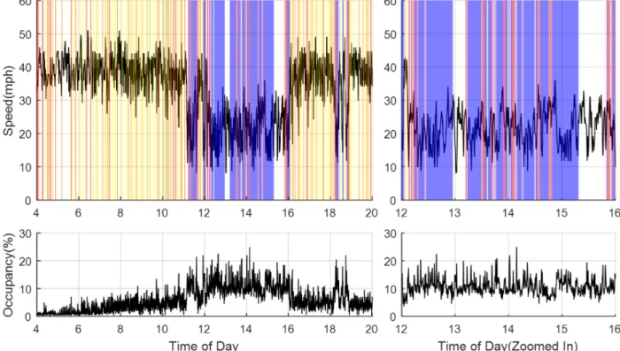
Figure 2.3 illustrates the events at the DMS sign on April 23, 2016, where the upper part shows the speed profile as a function of time and the lower part shows the sensor occupancy. Wavetronix sensor data are plotted using a black line, whereas the DMS information is represented by color-coded blocks — “Traffic Delay Ahead” messages are in yellow, “Slow Traffic Ahead” are in red, purple areas represent “Stopped Traffic Ahead”, and no message was displayed in areas with no color.
Several performance issues can be identified from Figure 2.3. First, the current control logic generated many short messages, which are displayed when the blocks are very thin.
2.
. .
2016
Q1
January February March
Q2
April May June
Q3 July 31 4 12 17 21 25 29 5 9 13 17 21 25 29 3 7 11 25 3 7 11 16 20 24 29 3 8 12 16 21 25 29 3 7 11 15 3 7 11 0 100 200 300 Tot 0 100 200 300 Sh 0 100 200 300 Clu
Second, many clustered messages exist, as shown by the alternating colored blocks (for example, in the region of 10:00 a.m.). The current DMS control logic did not properly function in some situations when it should have displayed a certain message but did not do so. The right side of Figure 2.3 is a zoomed-in version between noon and 4:00 p.m., when the speeds were
significantly slow (around 20 mph) with high traffic occupancy. However, no message was displayed at 1:00 and 3:30 p.m. under these congested conditions. This analysis suggests the need for continued development in some areas, as proposed in the following section.
2.2 Variable Advisory Speed Limit Sign in Severe Weather
The second traffic speed control device is a variable advisory speed limit system that reports severe winter weather, where the study area was a commuter corridor on Interstate 35 in central Iowa. The posted speed limit along this rural highway segment is 70 mph and it was evaluated under multiple winter snow conditions. The current system was run in ghost mode (operated in background without displaying any visual messages), which enabled researchers to rate the messages generated from the logic before deploying them to the public. Three types of message were created — Advised 55 mph, Advised 45 mph, and Advised 35 mph — which were archived using the Iowa DOT’s Advanced Traffic Management System (ATMS) software.
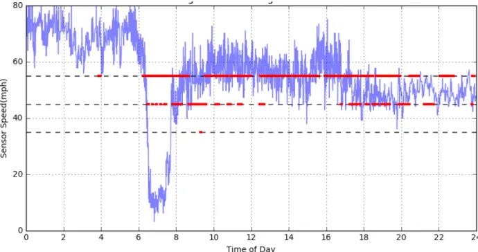
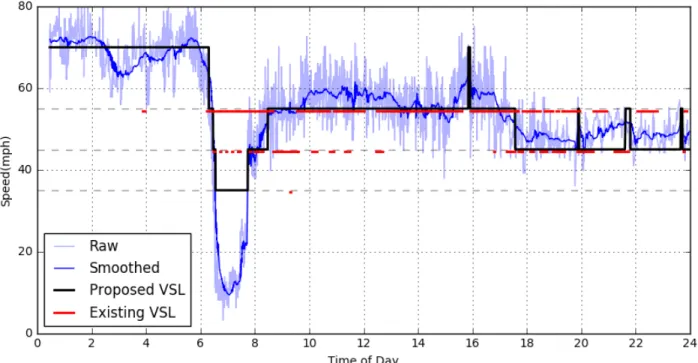
The existing system that displays advisory message was not designed to handle the complex nature of a transportation system and did not perform as expected or desired. The performance of the sign is visualized in Figure 2.4, where the horizontal axis represents the time of day and the vertical axis represents the raw Wavetronix sensor speed. The three reference speed limits are shown as dashed lines (55 mph, 45 mph, and 35 mph), and the solid red lines represent messages that would have been displayed on a dynamic advisory message board. Figure 2.4 indicates opportunities for enhancement, especially from 6 a.m. to 8 a.m., when the observed traffic speed had already reduced to ~10 mph due to the heavy snow but the existing control logic continued to display messages of 55 mph or 45 mph. To address such phenomena recognized, this dissertation research proposes a logic that can provide a realistic, reliable, and real-time advisory speed limit in response to winter weather conditions.
Figure 2.4 Performance of Existing Control Logic
2.3 Problem Statement
Figure 2.3 and Figure 2.4 illustrated the performance of the existing changeable message sign (CMS) applications in Iowa, which were less than desirable and suggest opportunities for improvement. To fully utilize the existing traffic sensor resources and build a data-driven CMS application, several problems are specified in the next several paragraphs, including data smoothing and labels for traffic incidents.
2.3.1 Data Smoothing
To identify the prevailing traffic conditions, traffic data quality (in terms of travelling speed and volume) is critical; however, sensor readings always have inherent noise. Two frequency-based filters — Fourier and wavelet transforms — can be applied to remove data
noise. A Fourier transform decomposes the original data into multiple sinusoidal functions, whereas a wavelet transform is based on the mother wavelet. By decomposing original data into sine/cosine signals, the Fourier transform is a great tool for analyzing stationary signals.
However, when data are not stationary, a wavelet transform is more useful because the mother wavelet enables changes in the property of data over time (Sifuzzaman et al., 2009)
For this study, a hard threshold that eliminates all coefficients greater than a pre-defined threshold (Thompson, 2014) was used to remove noise. The coefficients are given by the parameters in equation 1:
𝑥𝑥
(1)
where Coefi is the ith coefficient and λ is the hard threshold, which is defined as λ = kσ, with k as
the scaling parameter. For a given time series with N values using zero indexing, the estimated variance can be calculated using the following equation 2 (Thompson, 2014)(Gasser et al.,1986).
𝑥𝑥
(2)
where yi is the transformed value of the time series recorded at the time index i; yi-1 is the
transformed value of the time series recorded at the previous time step; and yi+1 is the
transformed value of the time series recorded at the subsequent time step.
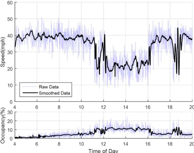
For the application of the dynamic messages, real-time noise filtering was performed. Therefore, the data were treated as though they had been received in a streaming manner. To address this issue, this study employed a sliding window approach for data smoothing, where the sliding window applied a small subset of recent historical data (previous 20 minutes). Figure 2.5 illustrates the raw data (for comparison with the same dataset given in Figure 2.3) and smoothed
sensor data, where the raw sensor data are denoted by a light blue color and the solid black line represents the smoothed data based on the Haar wavelet transform.
Figure 2.5 Data Smoothing
2.3.2 Labels for Changeable Messages
Unsupervised learning algorithms are designed for an unmarked dataset, whereas supervised learning algorithms are based on labeled data. Obtaining a labeled dataset is
expensive and time-consuming. One approach for handling a set of unlabeled data is to apply an unsupervised algorithm to identify clustered results and use these results in the subsequent supervised classification tasks (Coates & Ng, 2012). Similar to this concept, the author of this
study applied k-means clustering to cluster unlabeled traffic sensor data into several groups. The k-means clustering results can help experts assign these groups to different changeable messages, which can subsequently be used as labels. Based on the preprocessed dataset, a supervised
learning method was subsequently employed to replicate experts’ engineering judgment, which enabled the proposed control logic to automatically map the new data to a proper message for display as sensor data was streamed.
An unsupervised method aims to obtain a function that provides a compact description of a dataset. k-means clustering was employed in this paper to cluster traffic sensor data into k groups, where the difference within the same group is minimized and the difference between groups is maximized (Hastie et al., 2009). The determination of the number k is application-based. For example, for the DMS in the work zone application, the Iowa DOT had three different congestion statuses that were preferred based on the traffic conditions (“Delay”, “Slow Traffic”, and “Stopped Traffic”). Therefore, the data can be assumed to be divided into a maximum number of four different clusters, where the fourth cluster pertains to no message display. Regarding the variable advisory speed limit application during winter snow events, engineers recommended three different advisory speed limits based on traffic conditions: 55 mph, 45 mph, and 35 mph. As a result, four different clusters were defined for this application, where the 4th cluster pertains to the normal traffic condition.
After identifying the descriptive information from these clusters, experts manually assigned a label for each cluster based on their engineering judgment and used these labeled data for supervised classification. These labels included “Advised 55 mph Ahead”, “Advised 45 mph Ahead”, and “Advised 35 mph Ahead” for the variable advisory speed limit application. For the
DMS work zone application, the labels included “Traffic Delays Possible,” “Slow Traffic Ahead,” and “Stopped Traffic Ahead”.
A supervised method is similar to a function approximation, in which the algorithm formulates a function f based on a set of training <x, y> pairs. This generalized function f has the ability to map a new x as input to a proper output y. In the current application, the modeling input x represents smoothed speed (x1) and occupancy (x2), and y represents the proper message label
associated with <x1, x2>. Engineering judgment is the function f that is used to derive the label y
from the inputs. This function f, or engineering judgment, is extracted from the historical traffic events by the supervised method.
2.4 Summary
In this chapter, two changeable message signs in Iowa were assessed: the first type of CMS is the dynamic message sign in the I-74 work zone, and the second type of CMS is the variable advisory speed limit that reports severe winter weather. Due to noisy sensor readings and inappropriate message classification, their performance is not desirable. In the next section, the author applied data-driven techniques to enhance the performance and developed several applications to better manage traffic speeds in a real-time setting. One of the engineering solutions has been adopted and implemented by the Iowa Department of Transportation. This application monitors Iowa work zones 24/7 and sends out text multimedia messages when traffic congestion occurs.
CHAPTER 3. APPLICATIONS
The previous chapter identified several issues that deteriorate the performance of the existing traffic speed control applications in Iowa. In this chapter, after introducing the general framework of the application pipeline, different traffic speed control solutions are presented.
3.1 Introduction to Application Pipeline
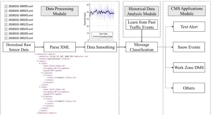
The application pipeline is shown in Figure 3.1 and contains three modules: (1) real-time data processing module, (2) historical data analysis module, and (3) changeable message sign (CMS) applications module. The application framework is written in Java with a Weka data mining package for message classification (Witten & Frank, 2016), JWave for wavelet data smoothing (Scheiblich, 2017), the TransSuite® ATMS web service for posting proper messages to field CMS signs, and Twilio REST API for multimedia text message alerts.
3.1.1 Data Processing Module
To address the problem of noisy sensor reading and identify predominant traffic patterns, the sensor raw data must be processed before sending the data to any decision-making stages. Iowa DOT monitors more than 500 permanent and temporary Wavetronix radar sensors
throughout the state, and traffic data can be accessed from these sensors via XML feeds with an update rate of 20 seconds. The author developed a series of Java scripts to automatically
download and parse XML data feeds 24/7, including XPath to quickly extract the target sensor information and a DOM parser to aggregate traffic data at certain locations. Once the structured data were formatted, real-time data smoothing was conducted using a sliding window. The need
for data smoothing was demonstrated in the previous section on the problem statement, and the sample smoothing results are illustrated in Figure 2.5 and Figure 3.1.
Figure 3.1 Application Pipeline
3.1.2 Historical Data Analysis Module
The second identified problem is the lack of labeled datasets for traffic events. This problem is addressed in the Historical Data Analysis module, which involves the process of analyzing data on past traffic events. Different applications may need a specific traffic dataset for support; however, they share the same principle. First, a person needs to pinpoint raw sensor data with targeted traffic events and apply a smoothing algorithm to the data. Second, the event data need to be clustered to help traffic engineers assign appropriate message labels. Finally, a supervised leaning method is applied to model these labeled datasets, and the results are
employed for real-time message classification. To demonstrate the application pipeline, the succeeding section considers the work zone DMS application as an example.
Iowa DOT engineers determined that three types of messages would be displayed on field DMS signs for different traffic congestion levels: delayed, slowed, and stopped traffic
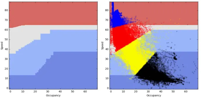
conditions. Following their requirement, multiple types of historical traffic event data in Iowa work zones were collected, including normal operation, traffic congestion, traffic accident, and work zone construction. The author applied unsupervised k-means to cluster work zone data into four groups, which helps DOT traffic engineers assign proper labels. Because there are only four categories of messages to display, one of the supervised classification methods—the decision tree—was chosen to replicate experts’ engineering judgement. Figure 3.2 shows the trained results for the DMS work zone application, where the x-axis is the smoothed sensor occupancy and the y-axis is the smoothed traffic speed. The domain is color-coded into four different regions that represent the DMS region: from top to bottom, normal conditions with no message display, “Traffic Delay Possible,” “Slow Traffic Ahead,” and “Stopped Traffic Ahead”. An overlay with the labeled data points is shown in the plot on the right. To avoid overfitting and achieve better generalization, the accuracy was not 100%, as illustrated by the misclassified labeled points in different color regions.
Figure 3.2 Labels and Decision Boundaries for DMS in Work Zone
3.2 Application Demo
Once the classified traffic condition is ready, different applications can be built. In this section, several applications are discussed, including 1) DMS in the I-74 bridge repair work zone, 2) variable advisory speed limit in snow events, 3) text alert in Iowa work zones, and some extensions based on the current research. In addition, a performance comparison between the existing system and the proposed application is provided.
3.2.1 DMS in I-74 Bridge Repair Work Zone
The existing DMS work zone, which displays messages, uses a nearby traffic sensor to measure speed or occupancy and some fixed thresholds to post messages that warn drivers of traffic congestion. Based on the field observation in Figure 2.3, these simplistic control methods
generate a significant number of very short messages, erroneous messages, and clusters of messages that continuously alternate among different displays.
Figure 3.3 shows the comparison between the proposed DMS control logic (bottom graphs) and the existing logic (upper graphs). The raw speed data and smoothed speeds are also plotted in light blue and black lines, respectively. In addition, a closer review of the period between noon and 4:00 p.m. is plotted on the right. The proposed logic improves the DMS performance, as evidenced by the reduction of the displayed short messages and the clustered messages. The logic successfully detected the period between noon and 4:00 p.m. by displaying desirable and stable messaging. To quantify the enhanced performance, the number of clustered messages, short-duration messages, and total displayed messages for the existing logic is 27, 90, and 268, respectively. The proposed control logic reduces these criteria to 15, 18, and 91 (for clustered, short, and total messages, respectively).
3.2.2 Variable Advisory Speed Limit in Snow Events
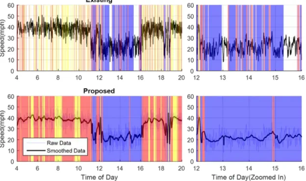
Comparisons between the proposed advised speed limit control logic (black line) and the existing logic (red line) for a weather event on December 28, 2015, are shown in Figure 3.4. The raw speed data and smoothed speed data using a wavelet transform are also plotted as a light blue line and a dark blue line, respectively. For the three performance measures, the proposed logic yielded zero clusters, zero short messages, and 15 total messages, compared with 12 clusters, 27 short messages, and 120 total messages generated by the existing logic.
A closer review of the period between 6 a.m. and 8 a.m., which experienced a steep speed reduction due to a severe snow event, reveals that the advisory messaging was improved using the proposed logic. Although most drivers travelled at a speed below 20 mph, the existing logic continued to advise a speed limit of 45 or 55 mph. Conversely, the proposed logic correctly detected the severe traffic condition and provided a more reasonable advisory speed limit of 35 mph.
Additional before and after comparisons were conducted for different dynamic advisory messaging stations along the same study corridor on different dates; the results are listed in Table 3.1. In addition to the dynamic advisory messaging function, the zero short messages generated in the proposed control logic are explained by the display time constraint that was implemented (each message was to be displayed for at least two minutes) to avoid short-duration messages.
Figure 3.4 Existing Logic and Proposed Control Logic
Table 3.1 Performance Comparisons between Proposed and Existing Logic
Proposed/(Existing) Station ID, Date Cluster Short Msg. Total
#1, Dec 24, 2015 1/(6) 0/(13) 23/(35) #1, Dec 28, 2015 0/(1) 0/(2) 14/(33) #2, Dec 24, 2015 0/(1) 0/(1) 13/(6) #2, Dec 28, 2015 1/(1) 0/(1) 22/(30) #3, Dec 24, 2015 1/(1) 0/(2) 13/(13) #3, Dec 28, 2015 0/(12) 0/(27) 13/(120) #4, Dec 24, 2015 0/(0) 0/(0) 3/(5) #4, Dec 28, 2015 0/(3) 0/(10) 12/(85)
After assessing the historical snow events in December 2015, the author implemented the proposed control logic and tested it in real time. The basic implementation logic followed the flow chart shown in Figure 3.1, including sensor XML data feed downloading, XML parsing, stream data smoothing, online classification, and sending out the classified message. The Iowa
DOT assigned several dummy DMS locations for testing; thus, the proposed advisory messaging control continued to run in “ghost” mode until approved. The real-time application was launched in winter 2017, during which several snow events occurred. To validate the accuracy of the real-time implementation, the generated dynamic advisory messages were compared with multiple data sources, including the roadway weather information sensor (surface friction), TransSuite TIS internal message logging report, roadway camera, and Wavetronix speed sensor.
3.2.2.1 Real-time implementation & validation example #1
The first snow event occurred on December 24, 2017, with snowy conditions from 1 a.m. to 11 a.m. Figure 3.5 shows the sensor data during the winter snow event near the location of 36th St. along I-35. The speed started to decrease at approximately 3 a.m., was approximately 50 mph from 5 a.m. to 8 a.m., and gradually returned to normal by noon. The friction conditions
illustrated a similar pattern — changed from the worst condition of snow warning/ice watch to the normal situation (wet and trace moisture, then dry). In the top plot of Figure 3.5, the light blue points represent the raw sensor data, and the solid blue line represents the smoothed speed that was used to trigger dynamic advisory messages (straight red line). The newly designed algorithm successfully displayed the message of “Advised 55 mph” from 3 a.m. to 7 a.m., which was verified using the TransSuite TIS Software Report in Figure 3.6.
Figure 3.5 Event #1 Speed Profile and Roadway Surface Condition
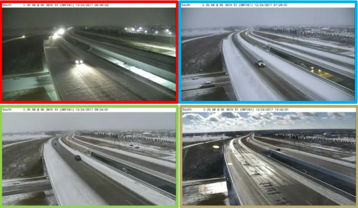
In addition to the quantitative description from the sensor/report, the author downloaded information from a nearby camera for better visualization. Figure 3.7 displays the camera view of the roadway surface environment for this location on the same day. From the top left to the bottom right, the conditions of snow warning, ice watch, wet, and trace moisture, respectively, are shown. The color that borders each camera image can also be related to the friction color shading in Figure 3.5, where the red area indicates “snow warning”, the blue block denotes “ice watch”, the green block represents “wet” conditions, and the gray block represents “trace moisture”.
3.2.2.2 Real-time implementation & validation example #2
Three days after the first event, another snowstorm occurred at night on December 27, 2017. This section illustrates the performance for this day. In addition to the winter weather advisory messaging, the system was capable of providing alerts for other severe traffic events, including traffic crashes.
Figure 3.8 shows the speed profile at 36th Street, where the red patched region indicates the snow warning logged by the roadway friction sensor. Although this snow weather event started at approximately 10 p.m., speeds began to decrease prior to this time due to the roadway surface conditions (Figure 3.9). The proposed logic detected this reduction in speeds at 10:20 p.m. (as verified via the TIS report in Figure 3.10) and displayed an advisory 55 mph message.
One highlight of this example is that the novel dynamic advisory messaging logic also correctly reacted to a traffic incident at approximately 3:30 p.m. The traffic conditions during this non-recurrent event are indicated on the right of Figure 3.8; the speed plummeted to 20 mph. A nearby camera’s imagery data were also retrieved to verify the algorithm’s accuracy, as
illustrated in Figure 3.11.
Figure 3.9 Event #2 Camera View of Roadway Conditions
Figure 3.11 Camera View of the Traffic Event on December 27, 2017
3.2.3 Text Alert in Iowa Work Zones
Providing dynamic messages to all roadway users is difficult and time-consuming due to various concerns, such as policy, budget, and right-of-way. Consequently, the variable advisory speed limit project continues to run in the background until it is approved. However, disclosing this information to a limited number of targeted personnel, such as district traffic engineers, operators in traffic management centers, and researchers, is easier. In this section, the application of text alerts in Iowa work zones resolves the dilemma faced by the variable advisory speed limit project. By continuously monitoring traffic information in real time, this text alert application enable DOT engineers to provide better/quicker response to traffic incidents.
This application takes the classified messages as inputs and sends out multimedia text messages to district engineers regarding severe traffic congestion. Figure 3.12 is an example of a
traffic congestion event, where the x-axis indicates time of day and the y-axis indicates traffic speed. Both the raw data (light gray dots) and the smoothed data (solid black line) are plotted with the displayed messages as different color blocks. Data from an entire day are shown in the left subplot, and a zoomed-in view of the traffic event is shown in the right subplot.
Figure 3.12 Example of Text Alert Application
DOT engineers only wanted to be informed of severe traffic situations, which was stopped condition traffic in this case, and wanted to limit the number of false calls that they received. Thus, this system applies a buffer of five minutes to avoid sending messages about abrupt traffic congestion; i.e., the text message is only sent to engineers if traffic is in a stopped condition for five continuous minutes. The accuracy of the message was a higher priority than the timeliness of the alerts. Two text message alerts were sent out per event: a text message alert was sent when a congested event was detected, and a follow-up text message alert was sent when the congestion cleared. The text message provided various pertinent information, including the timestamp, traffic speed, work zone name, milepost, and most importantly a snapshot from a nearby camera. The congestion clearance message included similar information and camera
imagery as well as details about the total congestion duration, for instance, 19 minutes in the example.
In the previously introduced work zone area, only one sensor is monitored. For the work zone with multiple sensors deployed, the message was triggered by the sensor with the worst traffic conditions. Figure 3.13 demonstrates another work zone operation with six sensors installed. Due to the length of the work zone area, some sensors did not experience congested traffic at the same time. To treat the system as a whole and notify the dedicated district traffic engineer, the program sent out a text message based on the sensor with the worst traffic
condition (red or gray lines). The example traffic incident occurred during the p.m. peak hours. Once a significant speed reduction was observed, a text alert was sent at 4:54 p.m. 51 minutes later, at 5:45 p.m., when normal traffic conditions resumed, a follow-up text was generated to advise people that the traffic incident had cleared.
Figure 3.13 Example of Text Alert Application with Multiple Sensors
The text alert application was launched at the beginning of June 2017 with 26 work zones and 66 sensors. Starting in May 2018, the operation has been scaled up to monitor 50 work zones with 350 sensors across the Iowa highway network. The system is functioning well, and positive
feedback has been received from the Iowa DOT. However, several issues have been identified. This application is highly dependent on the data quality from roadway sensors. If the sensor is not well calibrated, it will not work correctly due to the massive number of missing values, biased speed detections, and erroneous reading.
3.3 Extension Applications of the Current Research
Several other engineering solutions are feasible based on the author’s research findings. This section addresses two additional traffic engineering applications: the traffic data feed API integrated by the Iowa DOT traffic management center and the annual work zone performance report.
3.3.1 Traffic Management Center Data Feed API
The application pipeline was previously described in Figure 3.1, where the classified messages have multiple destinations. In addition to the three previously introduced applications (DMS in work zone, variable advisory speed limit reaction to winter snow event, and text alert system), the research team in the Iowa InTrans REACTOR lab developed a work zone alert data feed (http://reactorfeeds.org/) that continuously logs traffic information. The Iowa Traffic Management Center (TMC) subsequently integrated this data feed into their monitoring system and displayed the work zone traffic information in real time.
Figure 3.14 visualized this product, with a holistic view of the TMC room on the left and zoomed-in information highlighted on the right. This piece of information is almost the same as the information displayed in the text messages, including work zone name, sensor milepost, event activation time, and traffic conditions for an event. In contrast to the text message
application, which only focuses on severe traffic events, this TMC solution also tracks less severe events, i.e., congestion in Iowa highway work zones.
Figure 3.14 Operations Dashboard with Work Zone Alert Feed (Left Image from http://ia.zerofatalities.com/new-technologies-make-iowa-work-zones-safer/)
3.3.2 Work Zone Performance Evaluation
Work zone construction activities account for the majority of roadway congestion and potential sources of traffic accidents in Iowa and other states in the US. The Iowa State
University REACTOR Lab (https://reactor.ctre.iastate.edu/) provides an independent evaluation of work zone performance via the annual report of Traffic Critical Work Zone Evaluation. Prior to 2017, a simple fixed threshold of speed was used to identify traffic events in work zones, which encountered many false events. For the latest 2017 report, a data-driven approach was applied for better abnormal traffic incident detection and this detection technique is based on the condition boundaries defined in Figure 3.2.
In the performance report, a work zone event is defined as the traffic in slow or stop conditions. After processing all Wavetronix data during work zone seasons (March to October, 2017), 3,843 events were identified across 51 different work zones. Figure 3.15 is the map
visualization of these work zones. Once the list of identified events is ready, different work zone performance metrics are calculated based on the event start/end times, including congested hour and delay.
Figure 3.15 2017 Iowa Work Zone Map
Figure 3.16 utilizes the box plot to visualize the work zone performance in terms of event duration in minutes (y-axis). Work zone ID 6l-WB is highlighted (circled in Figure 3.15), with an average event time of approximately 1.5 hours. This work zone is the same work zone mentioned in the first DMS application for the I-74 bridge repair in Chapter 3.
Figure 3.16 2017 Iowa Work Zone Event Duration Boxplot
3.4 Summary
This chapter discussed three applications of changeable messages to better manage traffic speeds along an Iowa highway network. The discussion begins with dynamic message signs in the I-74 work zone, which is a proof of concept application based on a historical dataset. Then, the variable advisory speed limit was implemented in real time and successfully validated against other snow events in subsequent years. Due to various concerns, this application continues to run background without displaying any messages to the public. The text alert solution addressed the dilemma faced by dynamic advisory messaging, by exposing messages to dedicated personnel. This application continuously monitors 50 work zones in Iowa and sends out text messages with
a scene of the congested traffic incident. Based on the author’s current research results, two more applications have been developed by other members in the REACTOR lab.
So far, this dissertation research describes traffic speeds from a macroscopic viewpoint. However, how individual drivers react to traffic control devices cannot be sufficiently answered. In the following chapter, the author changes the angle to a smaller world and attempts to
CHAPTER 4. OLDER DRIVERS NATURALISTIC DRIVING STUDY
The previously discussed traffic speed analyses and applications were based on data collected by roadway sensors. Sensors comprise a valuable data source for monitoring traffic conditions in a highway network. However, these sensors collect data at fixed locations and cannot provide detailed individual-level driving information. With the development of sensor technology, additional instrumented vehicle data were collected using a different data source that enabled a driver’s speed to be evaluated from a micro perspective. In this chapter, the author conducts a naturalistic driving study to point out the driving patterns of older adults.
4.1 Introduction
Traditional traffic speed studies are based on the data collected by different types of roadway sensors, including but not limited to loop detectors, microwave sensors, inferred sensors, and ultrasonic sensors. Analyses based on these data describe the traffic characteristics from a macroscopic level. However, questions such as how an individual driver performs cannot be adequately answered. With the development of sensor technology, additional data on an individual level were collected. For example, Second Strategic Highway Research Program Naturalistic Driving Study (SHRP 2 NDS), which is led by the Virginia Tech Transportation Institute (VTTI) (Dingus et al., 2016), recruited more than 3,500 drivers and recorded a massive amount of continuous naturalistic driving data over three years. A 400-car naturalistic driving study from Australia (Regan et al., 2013) aims to understand interactions among drivers, vehicles, other road users, and roadway infrastructures. The University of Iowa targeted 100 older adult drivers (72 years old, on average) with the objective of building predictive models of
driver safety for older drivers (Dawson et al., 2010) (Emerson et al., 2012). In addition to various instrumented vehicle data, this older driver research provided a comprehensive list of personal-level predictors, including drivers’ motor function measures, visual perception assessments, and cognitive measures.
As an important component of a naturalistic driving study, an instrumented vehicle sensor system is an interdisciplinary field that consists of many other technologies, including telecommunications, roadway transportation, roadway safety, and sensor engineering. The system generated rich driving data (multiple in-vehicle sensors, dashboard camera videos, and GPS) that empowers many driver behavior studies.This type of study can improve roadway safety by identifying high-risk driving behaviors and different driving styles. For example, the VTTI built a probabilistic model to model crash probability based on SHRP 2 NDS data(Dingus et al., 2016). The model revealed a notable finding: drivers who were distracted more than 50% of the time were exposed to a much higher crash risk. Transportation safety can be significantly improved (4 million less crashes in the U.S.) if distractions to driving can be avoided. To detect the deviations from normal driving, Papazikou et al. (2017) analyzed the SHRP 2 data. They investigated multiple indicators, including braking, longitudinal/lateral acceleration, and time to collision, and validated the threshold for each indicator. They suggested several potential
indicators for better performance, such as traffic conditions, driver demographics, and yaw rates. In another driving style classification research, Vaitkus et al. (2014) used a k-nearest neighbors algorithm to classify aggressive driving and normal operations. Multiple features were tested, and the research indicated that the use of only the mean and median of the longitudinal and vertical acceleration can achieve reasonable classification results.
Naturalistic driving data are a great source for identifying different drivers due to their many practical applications, such as driving assistance devices and insurance pricing. SenseFleet is a platform that can identify different risky driving maneuvers and provide immediate feedback (Castignani et al., 2015). The system utilized fuzzy logic to obtain dynamic thresholds for
detecting events such as over-speed, acceleration braking, and vehicle steering. In addition to the data on vehicle dynamics, SenseFleet further integrated weather data for better driver behavior scoring. Van Ly et al. (2013) applied inertial sensor data to evaluate people’s driving styles. After analyzing multiple vehicle maneuvers, they determined that features of braking and turning movements were significant features for classifying different drivers. Another driver
identification study was conducted based on a single turn (Hallac et al., 2017). The study entailed a classification problem, in which the classifier can identify which individual driver was driving the car after a turning movement. They extracted data from 12 different in-vehicle sensors every 0.1 seconds and generated 12 features for each sensor reading. To reduce the dimensionality and avoid overfitting, a principle component analysis and random forest classifier were implemented. In the personal auto insurance industry, the current premium calculation models are general and are not customized for each individual driver (Husnjak et al., 2015). Vehicle telematics can identify different driving patterns, which enables usage-based insurance or a pay-as-you drive billing model. For example, the auto insurance carrier Progressive has adopted the SnapShot® device to collect driving behavior data for better/effective pricing.
4.2 Data Sources
This paper focuses on older adults’ driving behaviors that are associated with different roadway characteristics in Nebraska. To better understand various patterns of driving habits, the
author needs to integrate multiple data sources from in-vehicle sensor data, the Nebraska roadway information database, and drivers’ information.
4.2.1 Instrumented Vehicle Sensors
The University of Nebraska Medical Center (UNMC) manages a naturalistic driving study to identify patterns of driving behaviors of old adults. This study recruited drivers aged 65 to 92 years old (µ = 75 years old) and recorded their daily driving behaviors over three months. The dataset is comprehensive and uses multiple data sources:
• Global Positioning System (GPS) data: 5 Hz data, including longitude, latitude, GPS speed, heading, and satellite reception.
• On-Board Diagnostics (OBD) data: 5 Hz dataset containing the vehicle’s odometer reading, engine throttle, and engine revolutions per minute.
• Inertial Measurement Unit (IMU) data: 100 Hz dataset with three-axis accelerations (lateral, longitudinal, and vertical), yaw, roll, and pitch. Figure 4.1 shows the accelerometer data axes collected by the IMU.
• Dashboard cameras: a frontal view and cabin view combined video with 25 frames per second.
This large-scale dataset with 400 GB of structured text files (GPS, OBD, and IMU) and 7 TB of unstructured video files that can evaluate senior citizens’ driving behavior in many
aspects. Figure 4.2 provides a map of the driving routes of the participants during the period of study; a variety of colors represent the different subject drivers. All trips were centered in Omaha, Nebraska, because the recruited drivers live in this city. However, their travel
destinations were not limited to the Midwest; one participant even travelled to Canada. Due to the time constraints and the availability of roadway information files, this paper focuses on the GPS and IMU datasets for travel in Nebraska and uses other data sources for validation.
4.2.2 Nebraska Geographic Information System Database
Although every study vehicle was equipped with a frontal view dashboard camera, with numerous driving environment information available (roadway type, lane incursion, traffic signs, and weather), the deep learning objective detection model remains under development. Thus, this research enriched the GPS and IMU data with roadway information based on the Nebraska Geographic Information System (GIS) database, which logs data such as roadway functional classification, speed limit, roadway surface type, average daily traffic, and number of lanes. Figure 4.3 displays the Nebraska GIS shapefile with 355,138 polylines.
Figure 4.3 GIS Polyline Shapefile of Nebraska
4.2.3 Driver’s Information
The overarching goal of this naturalistic driving research led by UNMC is to measure real-life driving performance with respect to age-related cognitive dysfunction. Each driver was required to take a series of comprehensive examinations, and numerous predictors of driving behaviors of older drivers (Emerson et al., 2012) were collected:
• Cognitive assessment:
o COGSTAT: This score quantifies general cognition, which is a composite of several cognitive measures.
o Useful Filed of View (UFOV): UFOV was collected using personal computer touch screen to measure people’s processing speed, divided attention, and selective attention.
• Basic vision: Scores to quantify individual’s far visual acuity and contrast sensitivity.
• Movement ability:
o Get-up and go: the time in milliseconds required for a seated participant to stand up, walk 10 feet, turn around, and return to their seat (a smaller value suggests better performance).
o Functional reach: a clinical measure of balance that measures the starting position of a participant before he/she reaches forward (a larger value indicates better movement function).
• Speeding ticket record: The historical (two years before the driving study) speeding ticket record for each participant.
The dataset is sufficient for analyzing people’s driving behavior from a detailed perspective compared with roadway sensors. However, processing this dataset is challenging because the data are collected from different sensors and there is no universal key to merge them. In the next segment, different data wrangling techniques, including merging data from difference sources and filtering out noisy data points, are discussed.
4.3 Data Pre-Processing
GPS data and IMU data were merged based on timestamps. To handle the different sampling rates, 100 Hz IMU data are aggregated based on a 5 Hz GPS time. At GPS time t, the accelerometer data from IMU are averaged from t ± 0.1 seconds. Once the GPS data are merged, the longitude/latitude location can serve as the key to fuse with the Nebraska GIS database using Python’s geospatial package (GeoPandas). Drivers’ information was attached using the subject ID.
This paper aims to study old drivers’ driving behaviors with respect to different speed limits and other roadway features. Thus, drivers’ daily driving activities were divided into continuous three-minute trips for better visualization and analysis. Due to the complexity of driving environments, some trips’ data were not included in the final model, For example,
• Drivers made left/right/U-turn movements or stopped at intersections. When these
driving maneuvers occurred, a sudden reduction in speed can be observed from the speed trajectory. Since this paper focuses on driving behaviors with respect to different
roadway characteristics (primarily speed limit), these driving scenarios were not desired. Figure 4.4 provides one example of a driver making a right turn at an intersection. The subplot on the top is the speed profile, and subplot on the bottom indicates the trip location on the map. The speed of a driver significantly decreased when the driver
approached an intersection and intended to make a right turn. Once the driver finished the turning movement, the speed profile gradually reflected normal conditions.
Figure 4.4 Undesired Trips Example — Making Right Turn at an Intersection
• Trips that involved traffic congestion, work zone activities, traffic accidents, etc. These speed trajectories were often observed along high-speed roadways, where vehicles travel extremely slowly. Figure 4.5 displays a time series speed profile along a rural highway segment. Although the posted speed limit is 65 mph, the driver was travelling below 20 mph. By checking the dashboard camera, a traffic accident with a lane closure and police enforcement was identified.