esys User's guide: Solving partial differential equations with Escript and Finley. Release 3.0 (r2601)

(1)

esys

User’s Guide:

Solving Partial Differential Equations

with Escript and Finley

Release 3.0

(r2601)

Lutz Gross

et al.

(Editor)

Earth Systems Science Computational Centre (ESSCC)

School of Earth Sciences

The University of Queensland

Brisbane, Australia

Email:

[email protected]

(2)

School of Earth Sciences http://www.uq.edu.au/esscc Primary Business: Queensland, Australia Licensed under the Open Software License version 3.0

(3)

Abstract

esys.escriptis a python-based environment for implementing mathematical models, in particular those based on coupled, non-linear, time-dependent partial differential equations.

It consists of four major components • esys.escriptcore library

• finite element solver esys.finley(which uses fast vendor-supplied solvers or our paso linear solver library)

• the meshing interfaceesys.pycad • a model library.

The current version supports parallelization through both MPI for distributed memory and OpenMP for distributed shared memory. Theesys.pyvisimodule from previous releases has been deprecated. For more info on this and other changes from previous releases see Appendix A.2.

If you use this software in your research, then we would appreciate (but do not require) a citation. Some relevant references can be found in Appendix A.3.

(4)

(5)

Tutorial: Solving PDEs

1.1 Installation

To downloadescriptand friends , please visithttps://launchpad.net/escript-finley. The web site will offer binary distributions for some platforms and provide information about the installation process..

Please direct any questions you might have tomailto:[email protected].

1.2 The First Steps

In this chapter we give an introduction how to useesys.escriptto solve a partial differential equation (PDE ). We assume you are at least a little familiar with Python. The knowledge presented at the Python tutorial at http://docs.python.org/tut/tut.htmlis more than sufficient.

The PDE we wish to solve is the Poisson equation

−∆u=f (1.1)

for the solutionu. The functionf is the given right hand side. The domain of interest, denoted byΩ, is the unit square

Ω = [0,1]2={(x0;x1)|0≤x0≤1and0≤x1≤1} (1.2)

The domain is shown in Figure 1.1.

FIGURE1.1: DomainΩ = [0,1]2with outer normal fieldn.

∆denotes the Laplace operator, which is defined by

∆u= (u,0),0+ (u,1),1 (1.3)

(8)

where, for any functionuand any directioni,u,idenotes the partial derivative ofuwith respect toi.1 Basically, in the subindex of a function, any index to the left of the comma denotes a spatial derivative with respect to the index. To get a more compact form we will writeu,ij= (u,i),j which leads to

∆u=u,00+u,11= 2 X i=0

u,ii (1.4)

We often find that use of nestedP

symbols makes formulas cumbersome, and we use the more convenient Einstein summation convention . This drops theP

sign and assumes that a summation is performed over any repeated index. For instance we write

xiyi = 2 X i=0 xiyi (1.5) xiu,i= 2 X i=0 xiu,i (1.6) u,ii= 2 X i=0 u,ii (1.7) xijui,j = 2 X j=0 2 X i=0 xijui,j (1.8) (1.9) With the summation convention we can write the Poisson equation as

−u,ii= 1 (1.10)

wheref = 1in this example.

On the boundary of the domainΩthe normal derivativeniu,iof the solutionushall be zero, ie.ushall fulfill the homogeneous Neumann boundary condition

niu,i= 0. (1.11)

n= (ni)denotes the outer normal field of the domain, see Figure 1.1. Remember that we are applying the Einstein summation convention , i.eniu,i=n0u,0+n1u,1.2The Neumann boundary condition of Equation (1.11) should be fulfilled on the setΓN which is the top and right edge of the domain:

ΓN ={(x0;x1)∈Ω|x0= 1orx1= 1} (1.12) On the bottom and the left edge of the domain which is defined as

ΓD={(x0;x1)∈Ω|x0= 0orx1= 0} (1.13) the solution shall be identically zero:

u= 0. (1.14)

This kind of boundary condition is called a homogeneous Dirichlet boundary condition . The partial differential equation in Equation (1.10) together with the Neumann boundary condition Equation (1.11) and Dirichlet bound-ary condition in Equation (1.14) form a so called boundbound-ary value problem (BVP) for the unknown functionu. In general the BVP cannot be solved analytically and numerical methods have to be used construct an approxi-mation of the solutionu. Here we will use the finite element method (FEM). The basic idea is to fill the domain with a set of points called nodes. The solution is approximated by its values on the nodes. Moreover, the domain

1_{You may be more familiar with the Laplace operator being written as}_∇2_{, and written in the form} ∇2_u₌_∇t_{· ∇u}₌∂2u ∂x20 +∂ 2_u ∂x21 and Equation (1.1) as −∇2_u₌_f

2_{Some readers may familiar with the notation}∂u

∂n =niu,ifor the normal derivative.

(9)

FIGURE1.2: Mesh of4elements on a rectangular domain. Here each element is a quadrilateral and described by four nodes, namely the corner points. The solution is interpolated by a bi-linear polynomial.

is subdivided into smaller sub-domains called elements . On each element the solution is represented by a poly-nomial of a certain degree through its values at the nodes located in the element. The nodes and its connection through elements is called a mesh. Figure 1.2 shows an example of a FEM mesh with four elements in thex0and four elements in thex1direction over the unit square. For more details we refer the reader to the literature, for instance Reference [28, 5].

Theesys.escriptsolver we want to use to solve this problem is embedded into the python interpreter lan-guage. So you can solve the problem interactively but you will learn quickly that is more efficient to use scripts which you can edit with your favorite editor. To enter the escript environment you useescriptcommand3_:

escript

which will pass you on to the python prompt

Python 2.5.2 (r252:60911, Oct 5 2008, 19:29:17) [GCC 4.3.2] on linux2

Type "help", "copyright", "credits" or "license" for more information. >>>

Here you can use all available python commands and language features, for instance >>> x=2+3

>>> print "2+3=",x 2+3= 5

We refer to the python users guide if you not familiar with python.

esys.escriptprovides the classPoissonto define a Poisson equation . (We will discuss a more general form of a PDE that can be defined through theLinearPDEclass later). The instantiation of aPoissonclass object requires the specification of the domain Ω. In esys.escripttheDomainclass objects are used to describe the geometry of a domain but it also contains information about the discretization methods and the actual solver which is used to solve the PDE. Here we are using the FEM libraryesys.finley . The following statements create theDomainobjectmydomainfrom theesys.finleymethodRectangle

from esys.finley import Rectangle

mydomain = Rectangle(l0=1.,l1=1.,n0=40, n1=20)

In this case the domain is a rectangle with the lower, left corner at point(0,0) and the right, upper corner at

3_escript _{is not available under Windows yet.} _{If you run under windows you can just use the} _python _{command and the}

OMP NUM THREADSenvironment variable to control the number of threads.

(10)

(l0,l1) = (1,1). The argumentsn0andn1define the number of elements inx0andx1-direction respectively. For more details onRectangleand otherDomaingenerators within theesys.finleymodule, see Chapter 7. The following statements define thePoissonclass objectmypdewith domainmydomainand the right hand side

f of the PDE to constant1:

from esys.escript.linearPDEs import Poisson mypde = Poisson(mydomain)

mypde.setValue(f=1)

We have not specified any boundary condition but thePoissonclass implicitly assumes homogeneous Neuman boundary conditions defined by Equation (1.11). With this boundary condition the BVP we have defined has no unique solution. In fact, with any solutionuand any constantCthe functionu+Cbecomes a solution as well. We have to add a Dirichlet boundary condition . This is done by defining a characteristic function which has positive values at locationsx= (x0, x1)where Dirichlet boundary condition is set and0elsewhere. In our case ofΓD_{defined by Equation (1.13), we need to construct a function}_gammaD_{which is positive for the cases}_x

0= 0 orx1= 0. To get an objectxwhich contains the coordinates of the nodes in the domain use

x=mydomain.getX()

The methodgetXof theDomainmydomaingives access to locations in the domain defined bymydomain. The objectxis actually aDataobject which will be discussed in Chapter 3 in more detail. What we need to know here is that

xhas rank (number of dimensions) and a shape (list of dimensions) which can be viewed by calling thegetRank

andgetShapemethods:

print "rank ",x.getRank(),", shape ",x.getShape()

This will print something like rank 1, shape (2,)

TheDataobject also maintains type information which is represented by theFunctionSpaceof the object. For instance

print x.getFunctionSpace()

will print

Function space type: Finley_Nodes on FinleyMesh

which tells us that the coordinates are stored on the nodes of (rather than on points in the interior of) a

esys.finleymesh. To get thex0coordinates of the locations we use the statement x0=x[0]

Objectx0is again aDataobject now with rank0and shape(). It inherits theFunctionSpacefromx: print x0.getRank(),x0.getShape(),x0.getFunctionSpace()

will print

0 () Function space type: Finley_Nodes on FinleyMesh

We can now construct a functiongammaDwhich is only non-zero on the bottom and left edges of the domain with from esys.escript import whereZero

gammaD=whereZero(x[0])+whereZero(x[1])

whereZero(x[0])creates function which equals1 wherex[0]is (almost) equal to zero and0 elsewhere. Similarly,whereZero(x[1])creates function which equals1wherex[1]is equal to zero and0elsewhere. The sum of the results ofwhereZero(x[0])andwhereZero(x[1])gives a function on the domain mydo-mainwhich is strictly positive wherex0orx1is equal to zero. Note thatgammaDhas the same rank , shape and

FunctionSpacelikex0used to define it. So from

print gammaD.getRank(),gammaD.getShape(),gammaD.getFunctionSpace()

(11)

one gets

0 () Function space type: Finley_Nodes on FinleyMesh

An additional parameterqof thesetValuemethod of thePoissonclass defines the characteristic function of the locations of the domain where homogeneous Dirichlet boundary condition are set. The complete definition of our example is now:

from esys.linearPDEs import Poisson x = mydomain.getX()

gammaD = whereZero(x[0])+whereZero(x[1]) mypde = Poisson(domain=mydomain)

mypde.setValue(f=1,q=gammaD)

The first statement imports the Poissonclass definition from theesys.escript.linearPDEs module

esys.escriptpackage. To get the solution of the Poisson equation defined bymypdewe just have to call its

getSolution.

Now we can write the script to solve our Poisson problem from esys.escript import _*

from esys.escript.linearPDEs import Poisson from esys.finley import Rectangle

# generate domain:

mydomain = Rectangle(l0=1.,l1=1.,n0=40, n1=20) # define characteristic function of GammaˆD x = mydomain.getX()

gammaD = whereZero(x[0])+whereZero(x[1]) # define PDE and get its solution u mypde = Poisson(domain=mydomain) mypde.setValue(f=1,q=gammaD) u = mypde.getSolution()

The question is what we do with the calculated solutionu. Besides postprocessing, eg. calculating the gradient or the average value, which will be discussed later, plotting the solution is one one things you might want to do.

esys.escriptoffers two ways to do this, both base on external modules or packages and so data need to converted to hand over the solution. The first option is using thematplotlibmodule which allows plotting 2D results relatively quickly, see [12]. However, there are limitations when using this tool, eg. in problem size and when solving 3D problems. Thereforeesys.escriptprovides a second options based onVTKfiles which is especially designed for large scale and 3D problem and which can be read by a variety of software packages such asmayavi[2],VisIt[24].

1.2.1 Plotting Using

matplotlib

Thematplotlibmodule provides a simple and easy to use way to visualize PDE solutions (or otherData

objects). To hand over data fromesys.escripttomatplotlibthe values need to mapped onto a rectangular grid4_{. We will make use of the}_numpy_module.

First we need to create a rectangular grid. We use the following statements: import numpy

x_grid = numpy.linspace(0.,1.,50) y_grid = numpy.linspace(0.,1.,50)

x gridis an array defining the x coordinates of the grids whiley griddefines the y coordinates of the grid. In this case we use50points over the interval[0,1]in both directions.

Now the values created byesys.escriptneed to be interpolated to this grid. We will use thematplotlib mlab.griddatafunction to do this. We can easily extract spatial coordinates as alistby

4_{Users of Debian 5(Lenny) please note: this example makes use of the}_griddata_{method in}_{matplotlib.mlab}_{. This method is not}

part of version 0.98.1 which is available with Lenny. If you wish to use contour plots, you may need to install a later version. Users of Ubuntu 8.10 or later should be fine.

(12)

0.0 0.2 0.4 0.6 0.8 1.0 0.0 0.2 0.4 0.6 0.8 1.0

FIGURE1.3: Visualization of the Poisson Equation Solution forf= 1usingmatplotlib.

x=mydomain.getX()[0].toListOfTuples() y=mydomain.getX()[1].toListOfTuples()

In principle we can apply the sametoListOfTuplesmethod to extract the values from the PDE solutionu. However, we have to make sure that theDataobject we extract the values from uses the sameFunctionSpace

as we have us when extractingxandy. We apply theinterpolationtoubefore extraction to achieve this: z=interpolate(u,mydomain.getX().getFunctionSpace())

The values inzare now the values at the points with the coordinates given byxandy. These values are now interpolated to the grid defined byx gridandy gridby using

import matplotlib

z_grid = matplotlib.mlab.griddata(x,y,z,xi=x_grid,yi=y_grid )

z gridgives now the values of the PDE solutionuat the grid. The values can be plotted now using thecontourf: matplotlib.pyplot.contourf(x_grid, y_grid, z_grid, 5)

matplotlib.pyplot.savefig("u.png")

Here we use5contours. The last statement writes the plot to the file ‘u.png’ in the PNG format. Alternatively, one can use

matplotlib.pyplot.contourf(x_grid, y_grid, z_grid, 5) matplotlib.pyplot.show()

which gives an interactive browser window.

Now we can write the script to solve our Poisson problem from esys.escript import *

import numpy import matplotlib import pylab # generate domain:

gammaD = whereZero(x[0])+whereZero(x[1])

(13)

FIGURE1.4: Visualization of the Poisson Equation Solution forf= 1

# define PDE and get its solution u mypde = Poisson(domain=mydomain) mypde.setValue(f=1,q=gammaD) u = mypde.getSolution()

# interpolate u to a matplotlib grid: x_grid = numpy.linspace(0.,1.,50) y_grid = numpy.linspace(0.,1.,50) x=mydomain.getX()[0].toListOfTuples() y=mydomain.getX()[1].toListOfTuples() z=interpolate(u,mydomain.getX().getFunctionSpace()) z_grid = matplotlib.mlab.griddata(x,y,z,xi=x_grid,yi=y_grid ) # interpolate u to a rectangular grid:

matplotlib.pyplot.contourf(x_grid, y_grid, z_grid, 5) matplotlib.pyplot.savefig("u.png")

The entire code is available as ‘poisson matplotlib.py’ in the example directory. You can run the script using the

escriptenvironment

escript poisson_matplotlib.py

This will create the ‘u.png’, see Figure Figure 1.3. For details on the usage of thematplotlibmodule we refer to the documentation [12].

As pointed out,matplotlibis restricted to the two-dimensional case and should be used for small problems only. It can not be used underMPI as thetoListOfTuplesmethod is not safe underMPI5_.

1.2.2 Visualization using

VTK

As an alternativeescriptsupports the usage of visualization tools which base onVTK, eg. mayavi [2],VisIt[24]. In this case the solution is written to a file in theVTKformat. This file the can read by the tool of choice. Using

VTKfile isMPI safe.

To write the solutionuin Poisson problem to the file ‘u.xml’ one need to add the line saveVTK("u.xml",sol=u)

5_{The phrase ’safe under}_MPI_{’ means that a program will produce correct results when run on more than one processor under}_MPI_.

(14)

FIGURE1.5: Temperature Diffusion Problem with Circular Heat Source

The solutionuis now available in the ‘u.xml’ tagged with the name ”sol”. The Poisson problem script is now

from esys.escript import *

# generate domain:

gammaD = whereZero(x[0])+whereZero(x[1]) # define PDE and get its solution u mypde = Poisson(domain=mydomain) mypde.setValue(f=1,q=gammaD) u = mypde.getSolution() # write u to an external file saveVTK("u.xml",sol=u)

The entire code is available as ‘poisson VTK.py’ in the example directory

You can run the script using theescriptenvironment and visualize the solution usingmayavi:

escript poisson\hackscore VTK.py mayavi2 -d u.xml -m SurfaceMap

The result is shown in Figure Figure 1.4.

1.3 The Diffusion Problem

1.3.1 Outline

In this chapter we will discuss how to solve a time-dependent temperature diffusion PDE for a given block of material. Within the block there is a heat source which drives the temperature diffusion. On the surface, energy can radiate into the surrounding environment. Figure 1.5 shows the configuration.

In the next Section 1.3.2 we will present the relevant model. A time integration scheme is introduced to calculate the temperature at given time nodest(n). We will see that at each time step a Helmholtz equation must be solved. The implementation of a Helmholtz equation solver will be discussed in Section 1.3.3. In Section 1.3.4 the solver of the Helmholtz equation is used to build a solver for the temperature diffusion problem.

(15)

1.3.2 Temperature Diffusion

The unknown temperatureTis a function of its location in the domain and timet >0. The governing equation in the interior of the domain is given by

ρcpT,t−(κT,i),i=qH (1.15)

whereρcp andκare given material constants. In case of a composite material the parameters depend on their location in the domain. qH is a heat source (or sink) within the domain. We are using the Einstein summation convention as introduced in Chapter 1.2. In our case we assumeqHto be equal to a constant heat production rate

qcon a circle or sphere with centerxcand radiusrand0elsewhere:

qH(x, t) =    qc _k_x₋_xc_{k ≤}_r if 0 else (1.16)

for allxin the domain and all timet >0.

On the surface of the domain we are specifying a radiation condition which prescribes the normal component of the fluxκT,ito be proportional to the difference of the current temperature to the surrounding temperatureTref:

κT,ini=η(Tref −T) (1.17)

ηis a given material coefficient depending on the material of the block and the surrounding medium.niis thei-th component of the outer normal field at the surface of the domain.

To solve the time-dependent Equation (1.15) the initial temperature at timet= 0has to be given. Here we assume that the initial temperature is the surrounding temperature:

T(x,0) =Tref (1.18)

for allxin the domain. It is pointed out that the initial conditions satisfy the boundary condition defined by Equation (1.17).

The temperature is calculated at discrete time nodest(n)_where_t(0)_{= 0}_and_t(n)₌_t(n−1)₊_h_where_{h >}₀_{is the} step size which is assumed to be constant. In the following the upper index(n)refers to a value at timet(n)_{. The} simplest and most robust scheme to approximate the time derivative of the the temperature is the backward Euler scheme. The backward Euler scheme is based on the Taylor expansion ofT at timet(n)_:

T(n)≈T(n−1)+T_,t(n)(t(n)−t(n−1)) =T(n−1)+h·T_,t(n) (1.19) This is inserted into Equation (1.15). By separating the terms att(n)andt(n−1)one gets forn= 1,2,3. . .

ρcp h T (n)₋₍_κT(n) ,i ),i=qH+ ρcp h T (n−1) _(1.20) whereT(0)₌_T

refis taken form the initial condition given by Equation (1.18). Together with the natural boundary condition

κT_,i(n)ni=η(Tref −T(n)) (1.21)

taken from Equation (1.17) this forms a boundary value problem that has to be solved for each time step. As a first step to implement a solver for the temperature diffusion problem we will first implement a solver for the boundary value problem that has to be solved at each time step.

1.3.3 Helmholtz Problem

The partial differential equation to be solved forT(n)_{has the form}

ωT(n)−(κT_,i(n)),i=f (1.22) and we set ω=ρcp h andf =qH+ ρcp h T (n−1) . (1.23)

(16)

Withg=ηTref the radiation condition defined by Equation (1.21) takes the form

κT_,i(n)ni=g−ηT(n)onΓ (1.24)

The partial differential Equation (1.22) together with boundary conditions of Equation (1.24) is called the Helmholtz equation .

We want to use theLinearPDEclass provided byesys.escriptto define and solve a general linear,steady, second order PDE such as the Helmholtz equation. For a single PDE theLinearPDEclass supports the following form:

−(Ajlu,l),j+Du=Y . (1.25)

where we show only the coefficients relevant for the problem discussed here. For the general form of single PDE see Equation (4.1). The coefficientsA, andY have to be specified throughDataobjects in the general

FunctionSpaceon the PDE or objects that can be converted into suchDataobjects. Ais a rank-2Data

object andDandY are scalar. The following natural boundary conditions are considered onΓ:

njAjlu,l+du=y . (1.26)

Notice that the coefficientAis the same like in the PDE Equation (1.25). The coefficients dandy are each a scalarDataobject in the boundaryFunctionSpace. Constraints for the solution prescribing the value of the solution at certain locations in the domain. They have the form

u=rwhereq >0 (1.27)

randqare each scalarDataobject whereqis the characteristic function defining where the constraint is applied. The constraints defined by Equation (1.27) override any other condition set by Equation (1.25) or Equation (1.26). ThePoissonclass of theesys.escript.linearPDEsmodule, which we have already used in Chapter 1.2, is in fact a subclass of the more generalLinearPDEclass. Theesys.escript.linearPDEsmodule pro-vides aHelmholtzclass but we will make direct use of the generalLinearPDEclass.

By inspecting the Helmholtz equation (1.22) and boundary condition (1.24) and substitutinguforT(n)_{we can} easily assign values to the coefficients in the general PDE of theLinearPDEclass:

Aij =κδij D=ω Y =f

d=η y=g (1.28)

δij is the Kronecker symbol defined byδij = 1fori= jand0otherwise. Undefined coefficients are assumed to be not present.6 _{In this diffusion example we do not need to define a characteristic function} _q_{because the} boundary conditions we consider in Equation (1.24) are just the natural boundary conditions which are already defined in theLinearPDEclass (shown in Equation (1.26)).

The Helmholtz equation can be set up by following way7: mypde=LinearPDE(mydomain)

mypde.setValue(A=kappa*kronecker(mydomain),D=omega,Y=f,d=eta,y=g) u=mypde.getSolution()

where we assume thatmydomainis aDomainobject andkappa omega etaandgare given scalar values typ-icallyfloatorDataobjects. ThesetValuemethod assigns values to the coefficients of the general PDE. The

getSolutionmethod solves the PDE and returns the solutionuof the PDE.kroneckerisesys.escript

function returning the Kronecker symbol.

The coefficients can set by several calls ofsetValuewhere the order can be chosen arbitrarily. If a value is assigned to a coefficient several times, the last assigned value is used when the solution is calculated:

mypde=LinearPDE(mydomain)

mypde.setValue(A=kappa*kronecker(mydomain),d=eta) mypde.setValue(D=omega,Y=f,y=g)

mypde.setValue(d=2*eta) # overwrites d=eta u=mypde.getSolution()

6_{There is a difference in}_esys.escript_{of being not present and set to zero. As not present coefficients are not processed, it is more}

efficient to leave a coefficient undefined instead of assigning zero to it.

7_{Please, note that this is not a complete code. The complete code can be found in “helmholtz.py”.}

(17)

In some cases the solver of the PDE can make use of the fact that the PDE is symmetric where the PDE is called symmetric if

Ajl=Alj . (1.29)

Note thatD anddmay have any value and the right hand sidesY,yas well as the constraints are not relevant. The Helmholtz problem is symmetric. TheLinearPDEclass provides the methodcheckSymmetryto check if the given PDE is symmetric.

mypde=LinearPDE(mydomain)

mypde.setValue(A=kappa*kronecker(mydomain),d=eta) print mypde.checkSymmetry() # returns True

mypde.setValue(B=kronecker(mydomain)[0]) print mypde.checkSymmetry() # returns False mypde.setValue(C=kronecker(mydomain)[0]) print mypde.checkSymmetry() # returns True

Unfortunately, acheckSymmetryis very expensive and is recommendable to use for testing and debugging purposes only. ThesetSymmetryOnmethod is used to declare a PDE symmetric:

mypde = LinearPDE(mydomain)

mypde.setValue(A=kappa*kronecker(mydomain)) mypde.setSymmetryOn()

Now we want to see how we actually solve the Helmholtz equation. on a rectangular domain of lengthl0= 5and heightl1 = 1. We choose a simple test solution such that we can verify the returned solution against the exact answer. Actually, we takeT =x0(hereqH = 0) and then calculate the right hand side termsfandgsuch that the test solution becomes the solution of the problem. If we assumeκas being constant, an easy calculation shows that we have to choosef =ω·x0. On the boundary we getκniu,i=κn0. So we have to setg=κn0+ηx0. The following script ‘helmholtz.py’ which is available in the example directory implements this test problem using the

esys.finleyPDE solver:

from esys.escript import _*

from esys.escript.linearPDEs import LinearPDE from esys.finley import Rectangle

#... set some parameters ... kappa=1.

omega=0.1 eta=10.

#... generate domain ...

mydomain = Rectangle(l0=5.,l1=1.,n0=50, n1=10) #... open PDE and set coefficients ...

mypde=LinearPDE(mydomain) mypde.setSymmetryOn() n=mydomain.getNormal() x=mydomain.getX() mypde.setValue(A=kappa*kronecker(mydomain),D=omega,Y=omega*x[0], \ d=eta,y=kappa*n[0]+eta*x[0])

#... calculate error of the PDE solution ... u=mypde.getSolution()

print "error is ",Lsup(u-x[0]) saveVTK("x0.xml",sol=u)

To visualize the solution ‘x0. xml’ just use the command mayavi -d u.xml -m SurfaceMap &

and it is easy to see that the solutionT =x0is calculated.

The script is similar to the script ‘poisson.py’ discussed in Chapter 1.2.mydomain.getNormal()returns the outer normal field on the surface of the domain. The functionLsupimported by thefrom esys.escript import *statement and returns the maximum absolute value of its argument. The error shown by the print statement should be in the order of10−7_{. As piecewise bi-linear interpolation is used by}_esys.finley approx-imate the solution and our solution is a linear function of the spatial coordinates one might expect that the error would be zero or in the order of machine precision (typically≈ 10−15_{). However most PDE packages use an}

(18)

iterative solver which is terminated when a given tolerance has been reached. The default tolerance is10−8. This value can be altered by using thesetToleranceof theLinearPDEclass.

1.3.4 The Transition Problem

Now we are ready to solve the original time-dependent problem. The main part of the script is the loop over time

twhich takes the following form: t=0 T=Tref mypde=LinearPDE(mydomain) mypde.setValue(A=kappa*kronecker(mydomain),D=rhocp/h,d=eta,y=eta*Tref) while t<t_end: mypde.setValue(Y=q+rhocp/h*T) T=mypde.getSolution() t+=h

kappa,rhocp,etaandTrefare input parameters of the model.qis the heat source in the domain andhis the time step size. The variableT holds the current temperature. It is used to calculate the right hand side coefficientf in the Helmholtz equation in Equation (1.22). The statementT=mypde.getSolution()overwritesT with the temperature of the new time stept+h. To get this iterative process going we need to specify the initial temperature distribution, which equal toTref. TheLinearPDEclass objectmypdeand coefficients not changing over time are set up before the loop over time is entered. In each time step only the coefficientY is reset as it depends on the temperature of the previous time step. This allows the PDE solver to reuse information from previous time steps as much as possible.

The heat sourceqH which is defined in Equation (1.16) isqcin an area defined as a circle of radiusrand center

xcand zero outside this circle.q0is a fixed constant. The following script definesqHas desired: from esys.escript import length,whereNegative

xc=[0.02,0.002] r=0.001

x=mydomain.getX()

qH=q0*whereNegative(length(x-xc)-r)

xis a Dataclass object of the esys.escriptmodule defining locations in theDomain mydomain. The

length()imported from theesys.escriptmodule returns the Euclidean norm:

kyk=√yiyi =esys.escript.length(y) (1.30)

Solength(x-xc)calculates the distances of the locationxto the center of the circlexcwhere the heat source is acting. Note that the coordinates of xc are defined as a list of floating point numbers. It is automatically converted into aDataclass object before being subtracted fromx. The functionwhereNegativeapplied to

length(x-xc)-r, returns aDataobject which is equal to one where the object is negative (inside the circle) and zero elsewhere. After multiplication withqcwe get a function with the desired property of having valueqc

inside the circle and zero elsewhere.

Now we can put the components together to create the script ‘diffusion.py’ which is available in the example directory: :

from esys.escript.linearPDEs import LinearPDE from esys.finley import Rectangle

#... set some parameters ... xc=[0.02,0.002] r=0.001 qc=50.e6 Tref=0. rhocp=2.6e6 eta=75. kappa=240. tend=5.

# ... time, time step size and counter ...

(19)

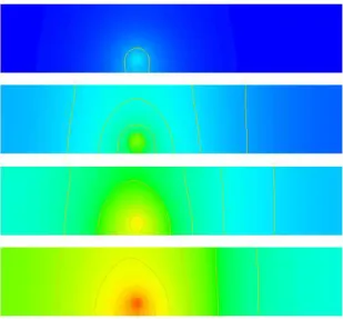
FIGURE1.6: Results of the Temperature Diffusion Problem for Time Steps1 16,32and48. t=0 h=0.1 i=0 #... generate domain ... mydomain = Rectangle(l0=0.05,l1=0.01,n0=250, n1=50) #... open PDE ... mypde=LinearPDE(mydomain) mypde.setSymmetryOn() mypde.setValue(A=kappa*kronecker(mydomain),D=rhocp/h,d=eta,y=eta*Tref) # ... set heat source: ....

x=mydomain.getX()

qH=qc*whereNegative(length(x-xc)-r) # ... set initial temperature .... T=Tref

# ... start iteration: while t<tend:

i+=1 t+=h

print "time step :",t

mypde.setValue(Y=qH+rhocp/h*T) T=mypde.getSolution()

saveVTK("T.%d.xml"%i,temp=T)

The script will create the files ‘T.1.xml’, ‘T.2.xml’,. . ., ‘T.50.xml’ in the directory where the script has been started. The files give the temperature distributions at time steps1,2,. . .,50in theVTKfile format.

Figure 1.6 shows the result for some selected time steps. An easy way to visualize the results is the command

mayavi -d T.1.xml -m SurfaceMap &

Use theConfigure Datawindow in mayavi to move forward and and backwards in time.

1.4 3-D Wave Propagation

In this next example we want to calculate the displacement field ui for any time t > 0 by solving the wave equation:

ρui,tt−σij,j= 0 (1.31)

(20)

-1 -0.8 -0.6 -0.4 -0.2 0 0.2 0.4 0.6 0.8 1 0 1 2 3 4 5

FIGURE1.7: Input Displacement at Source Point (α= 0.7,t0 = 3,U0= 1).

-10 -8 -6 -4 -2 0 2 4 6 8 10 0 1 2 3 4 5

FIGURE1.8: Input Acceleration at Source Point (α= 0.7,t0= 3,U0= 1).

in a three dimensional block of lengthLinx0 andx1 direction and heightH inx2direction. ρis the known density which may be a function of its location.σij is the stress field which in case of an isotropic, linear elastic material is given by

σij = λuk,kδij+µ(ui,j+uj,i) (1.32)

whereλandµare the Lame coefficients andδijdenotes the Kronecker symbol. On the boundary the normal stress is given by

σijnj= 0 (1.33)

for all timet >0.

Here we are modelling a point source at the pointxC in thex0-direction which is a negative pulse of amplitude

U0followed by the same positive pulse. In mathematical terms we use

u0(xC, t) =U0 √ 2(t−t0) α e 1 2− (t−t_{0 )}2 α2 _(1.34)

for allt≥0whereαis the width of the pulse andt0is the time when the pulse changes from negative to positive. In the simulations we will chooseα= 0.3andt0= 2, see Figure 1.7 and will apply the source as a constraint in a in a sphere of small radius around the pointxC.

(21)

We use an explicit time integration scheme to calculate the displacement fielduat certain time markst(n)where

t(n)=t(n−1)+hwith time step sizeh >0. In the following the upper index(n)refers to values at timet(n). We use the Verlet scheme with constant time step sizehwhich is defined by

u(n)= 2u(n−1)−u(n−2)+h2a(n) (1.35) (1.36) for alln= 2,3, . . .. It is designed to solve a system of equations of the form

u,tt=G(u) (1.37)

where one setsa(n)=G(u(n−1)). In our casea(n)_{is given by}

ρa(_in)=σ(_ij,jn−1) (1.38)

and boundary conditions

σ(_ijn−1)nj = 0 (1.39)

derived from Equation (1.33) where

σ_ij(n−1) = λu_k,k(n−1)δij+µ(u (n−1) i,j +u

(n−1)

j,i ). (1.40)

We also need to apply the constraint

a(₀n)(xC, t) =U0 p (2.) α2 (4 (t−t0)3 α3 −6 t−t0 α )e 1 2− (t−t_{0 )}2 α2 _(1.41)

which is derived from equation 1.34 by calculating the second order time derivative, see Figure 1.8. Now we have converted our problem for displacement,u(n)_{, into a problem for acceleration,}_a(n)_{, which now depends on the} solution at the previous two time steps,u(n−1)_and_u(n−2)_.

In each time step we have to solve this problem to get the accelerationa(n)_{, and we will use the}

LinearPDEclass of theesys.escript.linearPDEsto do so. The general form of the PDE defined through theLinearPDE

class is discussed in Section 4.1. The form which is relevant here is

Dija (n)

j =−Xij,j. (1.42)

The natural boundary condition

njXij = 0 (1.43)

is used. Withu=a(n)_{we can identify the values to be assigned to}_D_and_X_:

Dij =ρδij Xij =−σ

(n−1)

ij (1.44)

Moreover we need to define the locationrwhere the constraint 1.41 is applied. We will apply the constraint on a small sphere of radiusRaroundxC(we will use 3p.c. of the width of the domain):

qi(x) =

1 kx−xck ≤R

0 otherwise (1.45)

The following script defines a the functionwavePropagationwhich implements the Verlet scheme to solve our wave propagation problem. The argumentdomainwhich is a Domainclass object defines the domain of the problem. handtendare the time step size and the end time of the simulation. lam,muandrhoare material properties.

def wavePropagation(domain,h,tend,lam,mu,rho, x_c, src_radius, U0):

# lists to collect displacement at point source which is returned to the caller ts, u_pc0,u_pc1,u_pc2=[], [], [], []

x=domain.getX()

# ... open new PDE ... mypde=LinearPDE(domain)

(22)

mypde.getSolverOptions().setSolverMethod(mypde.getSolverOptions().LUMPING) kronecker=identity(mypde.getDim())

dunit=numpy.array([1.,0.,0.]) # defines direction of point source

mypde.setValue(D=kronecker*rho, q=whereNegative(length(x-xc)-src_radius)*dunit) # ... set initial values ....

n=0

# for first two time steps u=Vector(0.,Solution(domain)) u_last=Vector(0.,Solution(domain)) t=0

# define the location of the point source L=Locator(domain,xc)

# find potential at point source u_pc=L.getValue(u)

print "u at point charge=",u_pc

# open file to save displacement at point source u_pc_data=FileWriter(’./data/U_pc.out’)

ts.append(t); u_pc0.append(u_pc[0]), u_pc1.append(u_pc[1]), u_pc2.append(u_pc[2])

while t<tend: t+=h

# ... get current stress .... g=grad(u)

stress=lam*trace(g)*kronecker+mu*(g+transpose(g)) # ... get new acceleration ....

amplitude=U0*(4*(t-t0)**3/alpha**3-6*(t-t0)/alpha)*sqrt(2.)/alpha**2 \ *exp(1./2.-(t-t0)**2/alpha**2) mypde.setValue(X=-stress, r=dunit*amplitude)

a=mypde.getSolution()

# ... get new displacement ... u_new=2*u-u_last+h**2*a

# ... shift displacements .... u_last=u

u=u_new n+=1

print n,"-th time step t ",t u_pc=L.getValue(u)

print "u at point charge=",u_pc

# save displacements at point source to file for t > 0

ts.append(t); u_pc0.append(u_pc[0]), u_pc1.append(u_pc[1]), \

u_pc2.append(u_pc[2])

# ... save current acceleration in units of gravity and displacements if n==1 or n%10==0: saveVTK("./data/usoln.%i.vtu"%(n/10), \

acceleration=length(a)/9.81, displacement = length(u), \ tensor = stress, Ux = u[0] )

return ts, u_pc0, u_pc1, u_pc2

Notice that all coefficients of the PDE which are independent of timetare set outside thewhileloop. This is very efficient since it allows theLinearPDEclass to reuse information as much as possible when iterating over time.

The statement

mypde.getSolverOptions().setSolverMethod(mypde.getSolverOptions().LUMPING)

switches on the use of an aggressive approximation of the PDE operator as a diagonal matrix formed from the coefficientD. The approximation allows, at the cost of additional error, very fast solution of the PDE. When using lumping the presence ofA,BorCwill produce wrong results.

There are a few newesys.escriptfunctions in this example: grad(u)returns the gradientui,j of u(in factgrad(g)[i,j]==ui,j). There are restrictions on the argument of thegradfunction, for instance the statement

(23)

grad(grad(u))will raise an exception. trace(g)returns the sum of the main diagonal elementsg[k,k]of

gandtranspose(g)returns the matrix transpose ofg(ie.transpose(g)[i,j]=g[j,i]).

We initialize the values of u and u last to be zero. It is important to initialize both with the solution

FunctionSpace FunctionSpaceas they have to be seen as solutions of PDEs from previous time steps. In fact, thegraddoes not accept arguments with a certainFunctionSpace, for more details see Section 3.1.3. The Locator is designed to extract values at a given location (in this case xC) from functions such as the displacement vectoru. Typically theLocatoris used in the following form:

L=Locator(domain,xc) u=...

u_pc=L.getValue(u)

The return valueu pcis the value ofuat the locationxc8. The values are collected in the listsu pc0,u pc1

andu pc2together with the corresponding time marker ints. The values are handed back to the caller. Later we will show to ways to access these data.

One of the big advantages of the Verlet scheme is the fact that the problem to be solved in each time step is very simple and does not involve any spatial derivatives (which is what allows us to use lumping in this simulation). The problem becomes so simple because we use the stress from the last time step rather then the stress which is actually present at the current time step. Schemes using this approach are called an explicit time integration schemes . The backward Euler scheme we have used in Chapter 1.3 is an example of an implicit scheme . In this case one uses the actual status of each variable at a particular time rather then values from previous time steps. This will lead to a problem which is more expensive to solve, in particular for non-linear problems. Although explicit time integration schemes are cheap to finalize a single time step, they need significantly smaller time steps then implicit schemes and can suffer from stability problems. Therefore they need a very careful selection of the time step sizeh.

An easy, heuristic way of choosing an appropriate time step size is the Courant condition which says that within a time step a information should not travel further than a cell used in the discretization scheme. In the case of the wave equation the velocity of a (p-) wave is given asqλ+2_ρµ so one should choosehfrom

h= 1

5

r _ρ

λ+ 2µ∆x (1.46)

where∆xis the cell diameter. The factor1₅ is a safety factor considering the heuristics of the formula.

The following script uses thewavePropagationfunction to solve the wave equation for a point source located at the bottom face of a block. The width of the block in each direction on the bottom face is10km (x0andx1 directions ie. l0andl1). Thenegives the number of elements inx0andx1directions. The depth of the block is aligned with thex2-direction. The depth (l2) of the block in thex2-direction is chosen so that there are 10 elements and the magnitude of the of the depth is chosen such that the elements become cubic. We chose 10 for the number of elements inx2-direction so that the computation would be faster. Brick(n0, n1, n2, l0, l1, l2) is anesys.finleyfunction which creates a rectangular mesh with n0×n1 ×n2 elements over the brick

[0, l0]×[0, l1]×[0, l2].

from esys.finley import Brick

ne=32 # number of cells in x_0 and x_1 directions

width=10000. # length in x_0 and x_1 directions lam=3.462e9

mu=3.462e9 rho=1154. tend=60

U0=1. # amplitude of point source

# spherical source at middle of bottom face xc=[width/2.,width/2.,0.]

# define small radius around point xc src_radius = 0.03*width

print "src_radius = ",src_radius

mydomain=Brick(ne,ne,10,l0=width,l1=width,l2=10.*width/32.) h=(1./5.)*inf(sqrt(rho/(lam+2*mu))*inf(domain.getSize())

8_{In fact the finite element node which is closest to the given position. The usage of}_Locator_{is MPI save.}

(24)

FIGURE1.9: Selected time steps (n= 11,22,32,36) of a wave propagation over a10km×10km×3.125km block from a point source initially at(5km,5km,0)with time step sizeh= 0.02083. Color represents the displacement. Here the view is oriented onto the bottom face.

print "time step size = ",h

ts, u_pc0, u_pc1, u_pc2 = \

wavePropagation(mydomain,h,tend,lam,mu,rho,xc, src_radius, U0)

Thedomain.getSize()return the local element size∆x. Theinfmakes sure that the Courant condition 1.46 olds everywhere in the domain.

The script is available as ‘wave.py’ in the example directory . To visualize the results from the data directory:

mayavi2 -d usoln.1.vtu -m SurfaceMap &

You can rotate this figure by clicking on it with the mouse and moving it around. Again useConfigure Data

to move backwards and forward in time, and also to choose the results (acceleration, displacement orux) by using Select Scalar. Figure 1.9 shows the results for the displacement at various time steps.

It remains to show some possibilities to inspect the collected datau pc0,u pc1andu pc2. One way is to write the data to a file and then use an external package such asgnuplot[26], excel or OpenOffice to read the data for further analysis. The following code shows one possible form to write the data to the file ‘./data/U pc.out’: u_pc_data=FileWriter(’./data/U_pc.out’)

for i in xrange(len(ts)) :

u_pc_data.write("%f %f %f %f\n"%(ts[i],u_pc0[i],u_pc1[i],u_pc2[i])) u_pc_data.close()

TheU pc.outstores 4 columns of data:t, ux, uy, uzrespectively, whereux, uy, uzare thex0, x1, x2 compo-nents of the displacement vectoruat the point source. These can be plotted easily using any plotting package. In

gnuplot[26]the command:

plot ’U_pc.out’ u 1:2 title ’U_x’ w l lw 2, ’U_pc.out’ u 1:3 title ’U_y’ w l lw 2, ’U_pc.out’ u 1:4 title ’U_z’ w l lw 2

(25)

-1.5 -1 -0.5 0 0.5 1 1.5 0 2 4 6 8 10 U_x U_y U_z

FIGURE1.10: Amplitude at Point source from the Simulation.

will reproduce Figure 1.10 (As expected this is identical to the input signal shown in Figure 1.7)2. It is pointed out that we are not using the standardpythonopento write to the fileU pc.outas it is not safe when running

esys.escriptunder MPI, see chapter 2 for more details.

Alternatively, one can implement plotting the results at run time rather than in a post-processing step. This avoids the generation of an intermediate data file. Inescriptthe preferred way of creating 2D plots of time dependent data ismatplotlib. The following script creates the plot and writes it into the file ‘u pc.png’ in the PNG image format:

import matplotlib.pyplot as plt if getMPIRankWorld() == 0:

plt.title("Displacement at Point Source")

plt.plot(ts, u_pc0, ’-’, label="x_0", linewidth=1) plt.plot(ts, u_pc1, ’-’, label="x_1", linewidth=1) plt.plot(ts, u_pc2, ’-’, label="x_2", linewidth=1) plt.xlabel(’time’)

plt.ylabel(’displacement’) plt.legend()

plt.savefig(’u_pc.png’, format=’png’)

You can add the plt.show() to create a interactive browser window. Please not that through the

getMPIRankWorld() == 0statement the plot is generated on one processor only (in this case the rank 0 processor) when run under MPI.

Both options for processing the point source data are include in the example file ‘wave.py’. There other options available to process these data in particular through the SciPy[7] package , eg Fourier transformations. It is beyond the scope of this users guide to document the usage ofSciPy[7] for time series analysis but is highly recommended that users useSciPy[7] to any further data processing.

1.5 Elastic Deformation

(26)

In this section we want to examine the deformation of a linear elastic body caused by expansion through a heat distribution. We want a displacement fielduiwhich solves the momentum equation :

−σij,j= 0 (1.47)

where the stressσis given by

σij =λuk,kδij+µ(ui,j+uj,i)−(λ+

2

3µ)α(T−Tref)δij. (1.48)

In this formulaλandµare the Lame coefficients,αis the temperature expansion coefficient,Tis the temperature distribution andTrefa reference temperature. Note that Equation (1.47) is similar to Equation (1.31) introduced in section Section 1.4 but the inertia termρui,tthas been dropped as we assume a static scenario here. Moreover, in comparison to the Equation (1.32) definition of stressσin Equation (1.48) an extra term is introduced to bring in stress due to volume changes trough temperature dependent expansion.

Our domain is the unit cube

Ω ={(xi)|0≤xi≤1} (1.49)

On the boundary the normal stress component is set to zero

σijnj= 0 (1.50)

and on the face withxi= 0we set thei-th component of the displacement to0

ui(x) = 0 where xi= 0 (1.51) For the temperature distribution we use

T(x) =T0e−βkx−x c_k

; (1.52)

with a given positive constantβand locationxc_{in the domain.}

When we insert Equation (1.48) we get a second order system of linear PDEs for the displacementsuwhich is called the Lame equation. We want to solve this using theLinearPDEclass to this. For a system of PDEs and a solution with several components theLinearPDEclass takes PDEs of the form

−(Aijkluk,l),j =−Xij,j. (1.53)

Ais of rank-4Dataobject andX is of rank-2Dataobject. We show here the coefficients relevant for the we trying to solve. The full form is given in Equation (4.4). The natural boundary conditions take the form:

njAijkluk,l=njXij . (1.54)

Constraints take the form

ui=riwhereqi>0 (1.55)

randqare each rank-1Dataobject. We can easily identify the coefficients in Equation (1.53):

Aijkl=λδijδkl+µ(δikδjl+δilδjk) (1.56)

Xij = (λ+

2

3µ)α(T−Tref)δij (1.57)

(1.58) The characteristic functionqdefining the locations and components where constraints are set is given by:

qi(x) =

1 xi= 0

0 otherwise (1.59)

Under the assumption thatλ,µ,β andTref are constant we may useYi = (λ+2₃µ)α Ti. However, this choice would lead to a different natural boundary condition which does not set the normal stress component as defined in Equation (1.48) to zero.

(27)

Analogously to concept of symmetry for a single PDE, we call the PDE defined by Equation (1.53) symmetric if

Aijkl=Aklij (1.60)

(1.61) This Lame equation is in fact symmetric, given the difference inD anddas compared to the scalar case. The

LinearPDEclass is notified of this fact by calling itssetSymmetryOnmethod.

After we have solved the Lame equation we want to analyse the actual stress distribution. Typically the von–Mises stress defined by σmises= r 1 2((σ00−σ11) 2_{+ (}_σ 11−σ22)2+ (σ22−σ00)2) + 3(σ201+σ122 +σ220) (1.62) is used to detect material damage. Here we want to calculate the von–Mises and write the stress to a file for visualization.

The following script, which is available in ‘heatedbox.py’ in the example directory, solves the Lame equation and writes the displacements and the von–Mises stress into a file ‘deform.xml’ in theVTKfile format:

from esys.escript.linearPDEs import LinearPDE from esys.finley import Brick

#... set some parameters ... lam=1. mu=0.1 alpha=1.e-6 xc=[0.3,0.3,1.] beta=8. T_ref=0. T_0=1. #... generate domain ... mydomain = Brick(l0=1.,l1=1., l2=1.,n0=10, n1=10, n2=10) x=mydomain.getX() #... set temperature ... T=T_0*exp(-beta*length(x-xc)) #... open symmetric PDE ... mypde=LinearPDE(mydomain) mypde.setSymmetryOn() #... set coefficients ... C=Tensor4(0.,Function(mydomain)) for i in range(mydomain.getDim()): for j in range(mydomain.getDim()): C[i,i,j,j]+=lam C[j,i,j,i]+=mu C[j,i,i,j]+=mu msk=whereZero(x[0])*[1.,0.,0.] \ +whereZero(x[1])*[0.,1.,0.] \ +whereZero(x[2])*[0.,0.,1.] sigma0=(lam+2./3.*mu)*alpha*(T-T_ref)*kronecker(mydomain) mypde.setValue(A=C,X=sigma0,q=msk) #... solve pde ... u=mypde.getSolution()

#... calculate von-Misses stress g=grad(u)

sigma=mu*(g+transpose(g))+lam*trace(g)*kronecker(mydomain)-sigma0

sigma_mises=sqrt(((sigma[0,0]-sigma[1,1])**2+(sigma[1,1]-sigma[2,2])**2+ \ (sigma[2,2]-sigma[0,0])**2)/2. \

+3*(sigma[0,1]**2 + sigma[1,2]**2 + sigma[2,0]**2)) #... output ...

saveVTK("deform.xml",disp=u,stress=sigma_mises)

Finally the the results can be visualize by calling

mayavi -d deform.xml -f CellToPointData -m VelocityVector -m SurfaceMap &

(28)

FIGURE1.11: von–Mises Stress and Displacement Vectors.

Note that the filter CellToPointData is applied to create smooth representation of the von–Mises stress. Figure 1.11 shows the results where the vertical planes showing the von–Mises stress and the horizontal plane shows the vector representing displacements.

1.6 Stokes Flow

In this section we will look at Computational Fluid Dynamics (CFD) to simulate the flow of fluid under the influence of gravity. The StokesProblemCartesian class will be used to calculate the velocity and pressure of the fluid. The fluid dynamics is governed by the Stokes equation. In geophysical problems the velocity of fluids are low; that is, the inertial forces are small compared with the viscous forces, therefore the inertial terms in the Navier-Stokes equations can be ignored. For a body force,f, the governing equations are given by:

∇ ·(η(∇~v+∇T_~_v₎₎_{− ∇}_p₌₋_f,

(1.63) with the incompressibility condition

∇ ·~v= 0. (1.64)

wherep,ηandf are the pressure, viscosity and body forces, respectively. Alternatively, the Stokes equations can be represented in Einstein summation tensor notation (compact notation):

−(η(vi,j+vj,i)),j−p,i=fi, (1.65) with the incompressibility condition

−vi,i= 0. (1.66)

The subscript commaidenotes the derivative of the function with respect toxi. The body forcef in Equation (1.65) is the gravity acting in thex3direction and is given asf =−gρδi3. The Stokes equations is a saddle point problem, and can be solved using a Uzawa scheme. A class called StokesProblemCartesian in Escript can be used to solve for velocity and pressure; more detail on the class can be view in Chapter 6. In order to keep numerical stability, the time-step size needs to be kept below a certain value, to satisfy the Courant condition. The Courant number is defined as:

C= vδt

h . (1.67)

whereδt,v, andhare the time-step, velocity, and the width of an element in the mesh, respectively. The velocity

vmay be chosen as the maximum velocity in the domain. In this problem the time-step size was calculated for a Courant number of 0.4.

(29)

The following PYTHON script is the setup for the Stokes flow simulation, and is available in the example directory as ’fluid.py’. It starts off by importing the classes, such as the StokesProblemCartesian class, for solving the Stokes equation and the incompressibility condition for velocity and pressure. Physical constants are defined for the viscosity and density of the fluid, along with the acceleration due to gravity. Solver settings are set for the maximum iterations and tolerance; the default solver used is PCG. The mesh is defined as a rectangle, to represent the body of fluid. The gravitational force is calculated base on the fluid density and the acceleration due to gravity. The boundary conditions are set for a slip condition at the base of the mesh; fluid movement in the x-direction is free, but fixed in the y-direction. An instance of the StokesProblemCartesian is defined for the given computational mesh, and the solver tolerance set. Inside the while loop, the boundary conditions, viscosity and body force are initialized. The Stokes equation is then solved for velocity and pressure. The time-step size is calculated base on the Courant condition, to ensure stable solutions. The nodes in the mesh are then displaced based on the current velocity and time-step size, to move the body of fluid. The output for the simulation of velocity and pressure is then save to file for visualization.

from esys.escript import * import esys.finley

from esys.escript.linearPDEs import LinearPDE

from esys.escript.models import StokesProblemCartesian

#physical constants eta=1.0 rho=100.0 g=10.0 #solver settings tolerance=1.0e-4 max_iter=200 t_end=50 t=0.0 time=0 verbose=True #define mesh H=2.0 L=1.0 W=1.0

mesh = esys.finley.Rectangle(l0=L, l1=H, order=2, n0=20, n1=20) coordinates = mesh.getX() #gravitational force Y=Vector(0.0, Function(mesh)) Y[1]=-rho*g #element spacing h=Lsup(mesh.getSize())

#boundary conditions for slip at base

boundary_cond=whereZero(coordinates[1])*[0.0,1.0] #velocity and pressure vectors

velocity=Vector(0.0, ContinuousFunction(mesh)) pressure=Scalar(0.0, ContinuousFunction(mesh)) #Stokes Cartesian solution=StokesProblemCartesian(mesh) solution.setTolerance(tolerance) while t <= t_end:

print " --- Time step = %s ---"%( t ) print "Time = %s seconds"%( time )

solution.initialize(fixed_u_mask=boundary_cond,eta=eta,f=Y)

(30)

velocity,pressure=solution.solve(velocity,pressure,max_iter=max_iter, \ verbose=verbose)

print "Max velocity =", Lsup(velocity), "m/s"

#Courant condition

dt=0.4*h/(Lsup(velocity)) print "dt", dt

#displace the mesh

displacement = velocity * dt coordinates = mesh.getX()

mesh.setX(coordinates + displacement)

time += dt

vel_mag = length(velocity)

#save velocity and pressure output

saveVTK("vel.%2.2i.vtu"%(t),vel=vel_mag,vec=velocity,pressure=pressure) t = t+1.0

The results from the simulation can be viewed withmayavi, by executing the following command: mayavi -d vel.00.vtu -m SurfaceMap

Colour coded scalar maps and velocity flow fields can be viewed by selecting them in the menu. The time-steps can be swept through to view a movie of the simulation. Figures 1.12 and 1.13 shows the simulation output. Velocity vectors and a colour map for pressure are shown. As the time progresses the body of fluid falls under the influence of gravity. The view used here to track the fluid is the Lagrangian view, since the mesh moves with the fluid. One of the disadvantages of using the Lagrangian view is that the elements in the mesh become severely distorted after a period of time and introduce solver errors. To get around this limitation the Level Set Method can be used, with the Eulerian point of view for a fixed mesh.

(31)

(a) t=1 (b) t=20

(c) t=30

FIGURE1.12: Simulation output for Stokes flow. Fluid body starts off as a rectangular shape, then progresses downwards under the influence of gravity. Color coded distribution represents the scalar values for pressure. Velocity vectors are displayed at each node in the mesh to show the flow field. Computational mesh used was 20×20 elements.

(32)

(a) t=40

(b) t=50

(c) t=60

FIGURE1.13: Simulation output for Stokes flow.

(33)

CHAPTER

TWO

Execution of an

escript

Script

2.1 Overview

A typical way of starting yourescriptscript ‘myscript.py’ is with theescriptcommand1_: escript myscript.py

as already shown in section 1.22 _{. In some cases it can be useful to work interactively e.g. when debugging a} script, with the command

escript -i myscript.py

This will executemyscript.pyand when it completes (or an error occurs), apythonprompt will be provided. To leave the prompt pressControl-d.

To startescriptusing four threads (eg. if you use a multi-core processor) you can use escript -t 4 myscript.py

This will requireescriptto be compiled forOpenMP [18]. To startescriptusingMPI [14] with8processes you use

escript -p 8 myscript.py

If the processors which are used are multi–core processors or multi–processor shared memory architectures you can use threading in addition toMPI. For instance to run8MPI processes with using4threads each, you use the command

escript -p 8 -t 4 myscript.py

In the case of a super computer or a cluster, you may wish to distribute the workload over a number of nodes3. For example, to use8nodes, with4MPI processes per node, write

escript -n 8 -p 4 myscript.py

Since threading has some performance advantages over processes, you may specify a number of threads as well. escript -n 8 -p 4 -t 2 myscript.py

This runs the script on8nodes, with4processes per node and2threads per process.

1_The_escript_{launcher is not supported under}_{MS Windows}_yet.

2_{For this discussion, it is assumed that}_escript_{is included in your}_PATH_{environment. See installation guide for details.} 3_{For simplicity, we will use the term node to refer to either a node in a super computer or an individual machine in a cluster}

(34)

2.2 Options

The general form of theescriptlauncher is as follows:

escript

[

-nnn

] [

-pnp

] [

-tnt

] [

-fhostfile

] [

-x

] [

-V

] [

-e

] [

-h

] [

-v

] [

-o

] [

-c

] [

-i

] [

-b

] [

file

] [

ARGS

]

wherefileis the name of a script,ARGSare arguments for the script. Theescriptprogram will import your current environment variables. If nofileis given, then you will be given apythonprompt (see-ifor restrictions).

The options are used as follows:

-nnn the number of compute nodes nn to be used. The total number of process being used isnn·ns. This option overwrites the value of theESCRIPT NUM NODESenvironment variable. If a hostfile is given, the number of nodes needs to match the number hosts given in the host file. Ifnn >1butescriptis not compiled forMPI a warning is printed but execution is continued withnn= 1. If-nis not set the number of hosts in the host file is used. The default value is 1.

-pnp the number of MPI processes per node. The total number of processes to be used isnn·np. This option overwrites the value of theESCRIPT NUM PROCSenvironment variable. Ifnp>1butescriptis not compiled forMPI a warning is printed but execution is continued withnp= 1. The default value is 1. -tnt the number of threads used per processes. The option overwrites the value of the

ESCRIPT NUM THREADS environment variable. If nt > 1 but escript is not compiled for

OpenMP a warning is printed but execution is continued withnt= 1. The default value is 1.

-fhostfile the name of a file with a list of host names. Some systems require to specify the addresses or names of the compute nodes whereMPI process should be spawned. The list of addresses or names of the compute nodes is listed in the file with the namehostfile. If-n is set the the number of different hosts defined in

hostfilemust be equal to the number of requested compute nodesnn. The option overwrites the value of the ESCRIPT HOSTFILEenvironment variable. By default value no host file is used.

-c prints the information about the settings used to compileescriptand stops execution.. -V prints the version ofescriptand stops execution.

-h prints a help message and stops execution.

-i executes the scriptfileand switches to interactive mode after the execution is finished or an exception has occurred. This option is useful for debugging a script. The option cannot be used if more then one process (nn·np>1) is used.

-b do not invoke python. This is used to run non-python programs.

-e shows additional environment variables and commands used duringescriptexecution. This option is useful if users wish to execute scripts without using theescriptcommand.

-o switches on the redirection of output of processors with MPI rank greater than zero to the files ‘stdout r.out’ and ‘stderr r.out’ where ris the rank of the processor. The option overwrites the value of theESCRIPT STDFILESenvironment variable

-v prints some diagnostic information.

2.2.1 Notes

• Make sure thatmpiexecis in yourPATH.

• For MPICH and INTELMPI and for the case a hostfile is presentescriptwill start thempddemon before execution.

(35)

2.3 Input and Output

WhenMPI is used on more than one process (nn·np>1) no input from the standard input is accepted. Standard output on any process other the the master process (rank=0) will not be available. Error output from any processor will be redirected to the node whereescripthas been invoked. If the-oorESCRIPT STDFILESis set4_{, then} the standard and error output from any process other than the master process will be written to files of the names ‘stdout r.out’ and ‘stderr r.out’ (whereris the rank of the process).

If files are created or read by individualMPI processes with information local to the process (e.g in thedump

function) and more than one process is used (nn·np>1), theMPI process rank is appended to the file names. This will avoid problems if processes are using a shared file system. Files which collect data which are global for allMPI processors will created by the process withMPI rank 0 only. Users should keep in mind that if the file system is not shared, then a file containing global information which is read by all processors needs to be copied to the local file system beforeescriptis invoked.

2.4 Hints for MPI Programming

In general a script based on theesys.escriptmodule does not require modifications when running underMPI

. However, one needs to be careful if other modules are used.

WhenMPI is used on more than one process (nn·np>1) the user needs to keep in mind that several copies of his script are executed at the same time5 while data exchange is performed through theesys.escriptmodule. At any time,esys.escriptassumes that an argument of the typeint,float,strandnumpyhas an identical value across all processors. All values of these types returned byesys.escripthave the same value on all processors. If values produced by other modules are used as arguments the user has to make sure that the argument values are identical on all processors. For instance, the usage of a random number generator to create argument values bears the risk that the value may depend on the processor.

Special attention is required when using files on more then one processor as several processors access the file at the same time. Open a file for reading is safe, however the user has to make sure that the variables which are set from reading data from files are identical on all processors.

When writing data to a file it is important that only one processor is writing to the file at any time. As all values inesys.escriptare global it is sufficient to write values on the processor withMPI rank0only. The

FileWriterclass provides a convenient way to write global data to a simple file. The following script writes to the file’test.txt’on the processor with id0only:

from esys.escript import * f = FileWriter(’test.txt’) f.write(’test message’) f.close()

It is highly recommendable to use this class rather than the buildopenfunction as it will guarantee a script which will run in single processor mode as well as underMPI.

If there is the situation that on one of the processors is throwing an exception, for instance as opening a file for writing fails, the other processors are not automatically made aware of this asMPI is not handling exceptions. However,MPI will terminate the other processes but may not inform the user of the reason in an obvious way. The user needs to inspect the error output files to identify the exception.

4_{That is, it has a non-empty value.}

5_{In case of OpenMP only one copy is running but}_esys.escript_{temporarily spawns threads.}

(36)

(37)

CHAPTER

THREE

The Module

esys.escript

esys.escriptis a Python module that allows you to represent the values of a function at points in aDomain

in such a way that the function will be useful for the Finite Element Method (FEM) simulation. It also provides what we call a function space that describes how the data is used in the simulation. Stored along with the data is information about the elements and nodes which will be used byesys.finley.

In order to understand what we mean by the term ’function space’, consider that the solution of a partial differ-ential equation (PDE) is a function on a domainΩ. When solving a PDE using FEM, the solution is piecewise-differentiable but, in general, its gradient is discontinuous. To reflect these different degrees of smoothness, differ-ent function spaces are used. For instance, in FEM, the displacemdiffer-ent field is represdiffer-ented by its values at the nodes of the mesh, and so is continuous. The strain, which is the symmetric part of the gradient of the displacement field, is stored on the element centers, and so is considered to be discontinuous.

A function space is described by a FunctionSpaceobject. The following statement generates the object

solution spacewhich is aFunctionSpaceobject and provides access to the function space of PDE solutions on theDomainmydomain:

solution_space=Solution(mydomain)

The following generators for function spaces on aDomainmydomainare available: • Solution(mydomain): solutions of a PDE.

• ReducedSolution(mydomain): solutions of a PDE with a reduced smoothness requirement. • ContinuousFunction(mydomain): continuous functions, eg. a temperature distribution.

• Function(mydomain): general functions which are not necessarily continuous, eg. a stress field. • FunctionOnBoundary(mydomain): functions on the boundary of the domain, eg. a surface pressure. • FunctionOnContact0(mydomain): functions on side0of the discontinuity.

• FunctionOnContact1(mydomain): functions on side1of the discontinuity.

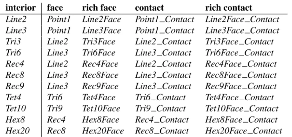
The reduced smoothness for PDE solution is often used to fulfill the Ladyzhenskaya-Babuska-Brezzi condition [11] when solving saddle point problems , eg. the Stokes equation. A discontinuity is a region within the domain across which functions may be discontinuous. The location of discontinuity is defined in theDomainobject. Figure 3.1 shows the dependency between the types of function spaces in Finley (other libraries may have different relationships).

The solution of a PDE is a continuous function. Any continuous function can be seen as a general function on the domain and can be restricted to the boundary as well as to one side of discontinuity (the result will be different depending on which side is chosen). Functions on any side of the discontinuity can be seen as a function on the corresponding other side.

A function on the boundary or on one side of the discontinuity cannot be seen as a general function on the domain as there are no values defined for the interior. For most PDE solver libraries the space of the solution and continuous functions is identical, however in some cases, eg. when periodic boundary conditions are used in

esys.finley, a solution fulfills periodic boundary conditions while a continuous function does not have to be periodic.

esys User's guide: Solving partial differential equations with Escript and Finley. Release 3.0 (r2601)

esys

User’s Guide:

Solving Partial Differential Equations

with Escript and Finley

Release 3.0

(r2601)

Lutz Gross

et al.

(Editor)

Earth Systems Science Computational Centre (ESSCC)

School of Earth Sciences

The University of Queensland

Brisbane, Australia

Email:

CONTENTS

ONE

Tutorial: Solving PDEs

1.1

Installation

1.2

The First Steps

1.2.1

Plotting Using

matplotlib

1.2.2

Visualization using

VTK

1.3

The Diffusion Problem

1.3.1

Outline

1.3.2

Temperature Diffusion

1.3.3

Helmholtz Problem

1.3.4

The Transition Problem

1.4

3-D Wave Propagation

1.5

Elastic Deformation

1.6

Stokes Flow

TWO

Execution of an

escript

Script

2.1

Overview

2.2

Options

[

] [

] [

] [

] [

] [

] [

] [

] [

] [

] [

] [

] [

] [

] [

]

2.2.1

Notes

2.3

Input and Output

2.4

Hints for MPI Programming

THREE

The Module

esys.escript