Efficient Robust Adaptive Beamforming Algorithms for Sensor Arrays

Algorithms for Sensor Arrays

Hang Ruan

Doctor of Philosophy

University of York

Electronics

March 2016

Sensor array processing techniques have been an important research area in recent years. By using a sensor array of a certain configuration, we can improve the parameter estima-tion accuracy from the observaestima-tion data in the presence of interference and noise. In this thesis, we focus on sensor array processing techniques that use antenna arrays for beam-forming, which is the key task in wireless communications, radar and sonar systems.

Firstly, we propose a low-complexity robust adaptive beamforming (RAB) technique which estimates the steering vector using a Low-Complexity Shrinkage-Based Mismatch Estimation (LOCSME) algorithm. The proposed LOCSME algorithm estimates the co-variance matrix of the input data and the interference-plus-noise coco-variance (INC) ma-trix by using the Oracle Approximating Shrinkage (OAS) method. Secondly, we present cost-effective low-rank techniques for designing robust adaptive beamforming (RAB) al-gorithms. The proposed algorithms are based on the exploitation of the cross-correlation between the array observation data and the output of the beamformer. Thirdly, we pro-pose distributed beamforming techniques that are based on wireless relay systems. Algo-rithms that combine relay selections and SINR maximization or Minimum Mean-Square-Error (MMSE) consensus are developed, assuming the relay systems are under total relay transmit power constraint. Lastly, we look into the research area of robust distributed beamforming (RDB) and develop a novel RDB approach based on the exploitation of the cross-correlation between the received data at the relays and the destination and a subspace projection method to estimate the channel errors, namely, the cross-correlation and subspace projection (CCSP) RDB technique, which efficiently maximizes the out-put SINR and minimizes the channel errors. Simulation results show that the proposed techniques outperform existing techniques in various performance metrics.

Abstract ii

Contents iii

List of Figures x

List of Tables xiii

Acknowledgements xv Declaration xvi 1 Introduction 1 1.1 Problem Statements . . . 1 1.2 Motivations . . . 2 1.3 Contributions . . . 3 1.4 Thesis Outline . . . 5 1.5 Notations . . . 6

2 Literature Review 9

2.1 Introduction . . . 9

2.2 Sensor Array Processing . . . 10

2.2.1 Uniform Linear Array . . . 10

2.2.2 Uniform Circular Array . . . 11

2.3 Beamforming . . . 11

2.3.1 MVDR Optimum Beamformer . . . 12

2.4 Adaptive Beamforming Algorithms . . . 13

2.4.1 MVDR-LMS Adaptive Algorithm . . . 14

2.4.2 MVDR-RLS Adaptive Algorithm . . . 15

2.4.3 MVDR-CG Adaptive Algorithm . . . 16

2.5 Robust Adaptive Beamforming . . . 18

2.5.1 Steering Vector Mismatch . . . 18

2.5.2 Existing RAB Algorithms . . . 20

2.6 Distributed Beamforming . . . 23

2.6.1 Distributed Beamforming and Wireless Relay Networks . . . 23

Consensus Approach . . . 27

2.6.4 Generalized Relay Networks with SNR Maximization Approaches 28 2.6.5 Distributed Beamforming with Relay Selection . . . 31

2.6.6 Robust Distributed Beamforming . . . 32

2.7 Summary . . . 33

3 Low-Complexity Shrinkage-Based Mismatch Estimation (LOCSME) Algo-rithms for Robust Adaptive Beamforming 34 3.1 Introduction . . . 35

3.1.1 Prior and Related Work . . . 35

3.1.2 Contributions . . . 36

3.2 System Model and Problem Statement . . . 37

3.3 Batch LOCSME Algorithm . . . 38

3.3.1 Steering Vector Estimation using LOCSME . . . 39

3.3.2 Interference-Plus-Noise Covariance Matrix Estimation . . . 40

3.4 Stochastic Gradient LOCSME Type Algorithm . . . 42

3.4.1 INC Matrix Estimation with a Knowledge-Aided Shrinkage Method 44 3.4.2 Adaptive Computations of Beamforming Weight Vector . . . 45

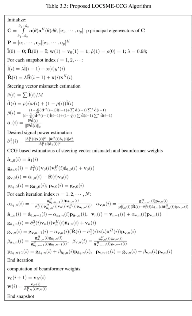
3.5.2 LOCSME-MCG algorithm . . . 48

3.6 Performance Analysis . . . 51

3.6.1 Shrinkage Analysis . . . 53

3.6.2 Complexity Analysis . . . 55

3.7 Simulations . . . 57

3.7.1 Mismatch due to Coherent Local Scattering . . . 57

3.7.2 Mismatch due to Incoherent Local Scattering . . . 59

3.8 Summary . . . 62

4 Orthogonal Krylov Subspace Projection Mismatch Estimation for Robust Adaptive Beamforming 63 4.1 Introduction . . . 63

4.1.1 Prior and Related Work . . . 64

4.1.2 Contributions . . . 64

4.2 System Model and Problem Statement . . . 66

4.3 Proposed OKSPME Method . . . 68

4.3.1 Desired Signal Power Estimation . . . 68

4.3.2 Orthogonal Krylov Subspace Approach for Steering Vector Mis-match Estimation . . . 70

4.4 Proposed Adaptive Algorithms . . . 73

4.4.1 OKSPME-SG Adaptive Algorithm . . . 73

4.4.2 OKSPME-CCG Adaptive Algorithm . . . 75

4.4.3 OKSPME-MCG Adaptive Algorithm . . . 77

4.5 Analysis . . . 80

4.5.1 MSE analysis . . . 82

4.5.2 Complexity Analysis . . . 89

4.6 Simulations . . . 90

4.6.1 Mismatch due to Coherent Local Scattering . . . 91

4.6.2 Mismatch due to Incoherent Local Scattering . . . 94

4.7 Summary . . . 97

5 Distributed Beamforming and Relay Selection Techniques 98 5.1 Introduction . . . 98

5.1.1 Prior and Related Work . . . 99

5.1.2 Contributions . . . 100

5.2 System Model . . . 100

5.3.2 Relay Selection . . . 105

5.4 Proposed Joint MSINR and RGSRS Algorithm . . . 105

5.5 Simulations . . . 108

5.6 Summary . . . 109

6 Robust Distributed Beamforming Techniques 111 6.1 Introduction . . . 111

6.1.1 Prior and Related Work . . . 112

6.1.2 Contributions . . . 112

6.2 System Model . . . 113

6.3 Proposed CCSP RDB Algorithm . . . 115

6.4 Analysis . . . 118

6.4.1 MSE Analysis . . . 118

6.4.2 Cross-Correlation and Subspace Projection Analysis . . . 122

6.5 Simulations . . . 126

6.6 Summary . . . 129

7 Conclusions and Future Work 131 7.1 Conclusions . . . 131

Glossary 135

2.1 Uniform Linear Array. . . 11

2.2 Uniform Circular Array . . . 12

2.3 Adaptive Beamformer. . . 14

2.4 Local Scattering Effect of Detecting a Moving Object from a Base Station Array . . . . 19

2.5 System Model of Relay Network . . . 24

3.1 Complexity versus number of sensors . . . 56

3.2 Coherent local scattering, SINR versus snapshots . . . 58

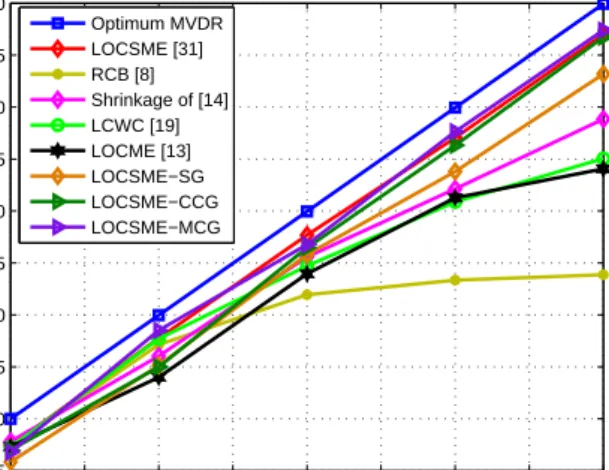
3.3 Coherent local scattering, SINR versus SNR . . . 58

3.4 coherent local scattering, SINR versus snapshots . . . 59

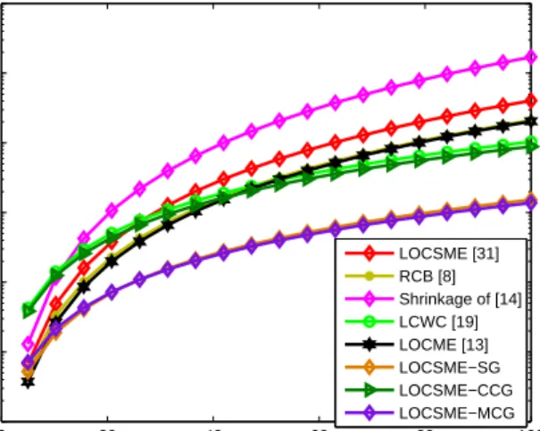
3.5 incoherent local scattering, SINR versus snapshots . . . 60

3.6 incoherent local scattering, SINR versus SNR . . . 60

3.7 Scenario with incoherent local scattering and time-varying DoAs . . . 61

4.3 Update scheme of the OKSPME method . . . 85

4.4 Complexity Comparison . . . 91

4.5 Coherent local scattering, SINR versus snapshots, M = 10, K = 3, INR = 20dB . . . 92

4.6 Coherent local scattering, SINR versus snapshots,M = 12,K = 3 . . . . 94

4.7 Coherent local scattering, SINR versus SNR,M = 12,K = 3 . . . 94

4.8 Coherent local scattering, SINR versus snapshots,M = 12 . . . 95

4.9 Coherent local scattering, SINR versus snapshots,M = 40,K = 3 . . . . 95

4.10 Coherent local scattering, SINR versus SNR,M = 40,K = 3 . . . 96

4.11 Incoherent local scattering, SINR versus SNR,M = 40,K = 3. . . 96

5.1 System model. . . 101

5.2 SINR versus SNR and M. . . 109

5.3 BER versus SNR. . . 109

6.1 MSE bounds versusλmax,k,σλ,k = 0.9λmax,k . . . 123

6.2 MSE bounds versusλmax,k,σλ,k = 0.5λmax,k . . . 123

6.3 SINR versus SNR,PT = 1dBW,max = 0.2, INR=10dB . . . 127

6.6 SINR versusPT, SNR=10dB,max = 0.5, INR=10dB . . . 129 6.7 SINR versus SNR,PT = 1dBW,max = 0.2, INR=20dB . . . 130 6.8 SINR versus snapshots,PT = 1dBW,max = 0.2, SNR=10dB, INR=20dB 130

3.1 Proposed LOCSME Algorithm . . . 43

3.2 Proposed LOCSME-SG Algorithm . . . 46

3.3 Proposed LOCSME-CCG Algorithm . . . 49

3.4 Proposed LOCSME-MCG Algorithm . . . 52

3.5 Complexity Comparison . . . 56

3.6 Changes of Interferers . . . 61

4.1 Arnoldi-modified Gram-Schmidt algorithm . . . 71

4.2 Proposed OKSPME method . . . 74

4.3 Proposed OKSPME-CCG algorithm . . . 78

4.4 Proposed OKSPME-MCG algorithm . . . 81

4.5 Complexity Comparison . . . 90

4.6 Changes of Interferers . . . 93

5.3 Complexity Comparison . . . 108

I would like to show great gratitude to my supervisors, Prof. Rodrigo C. de Lamare and Dr. Yury Zakharov for their support and guidance during my research, without which I would not be able to complete this work.

I’m also grateful to my family, who have been giving me both tremendous moral and financial support continuously and unwaveringly throughout my education, without which I would not achieve this far.

Finally, I would like to thank all my friends and colleagues in York and beyond, whose advice, friendship and goodwill has helped me immensely.

This work has not previously been presented for an award at this, or any other, University. All work presented in this thesis is original to the best knowledge of the author. Some of the research presented in this thesis has resulted in some publications, which are listed in section 1.6, the Publications section, which is the at the end of Chapter 1. References and acknowledgements to work by other researchers have been given as appropriate.

Introduction

Contents

1.1

Problem Statements

In important applications such as wireless communications, radar, sonar and biomedical processing, sensor array processing is indispensably and commonly used to filter signals in the space-time field by exploiting their spatial characteristics [1–3]. The advantages of sensor array processing include the following: the signal-to-interference-plus-noise ratio (SINR) is enhanced compared to using a single sensor, the directions of arrivals (DoAs) and waveforms of the emitted signal sources can be determined and parameters can be measured precisely in high dimensional spaces [1]. The main goal of sensor array signal processing is the estimation of parameters and extraction of information by fusing tem-poral and spatial information, captured via sampling a wavefield with a set of judiciously

placed sensors [1].

The topic we are particularly interested in sensor array processing is beamforming technique, which can be categorized as traditional or centralized beamforming and dis-tributed beamforming techniques. In traditional beamforming, we aim to combine the measurements from an antenna array to maximize its gain in a specific direction [1]. In distributed beamforming, we have a relay system which can be also treated as an array composed by a set of antenna elements with distributed locations. The relay nodes (or antennas) are also independent processing units if there is no cooperation among them-selves [88]. The advantages of distributed beamforming include an increase in the range of communications and a reduction in the network power consumptions, to overcome obstacles like poor channel and relay processing. However, estimation procedures of some crucial parameters like steering vectors, channel statistics and data covariance ma-trices can be challenging, especially if the implementations are considered under dynamic and unstable environments, which leads to the development of robust beamforming tech-niques. There has been an intensive research on robust beamforming methods, but still computational complexity and estimation precision are some unavoidable challenges.

1.2

Motivations

Both environmental effects and internal factors can affect the overall system performance. In traditional beamforming, the steering vector may suffer mismatch due to environmental uncertainties like look direction and pointing errors, source wavefront distortion, near-far field problem, signal fading and scattering, as well as non-environmental factors like im-perfect array calibration and distorted antenna shape [7]. In distributed beamforming, the channel state information (CSI) is normally unknown (mismatched) in practical scenar-ios, which may be caused by limited channel feedback or outdate channel states [80]. In order to mitigate the effects of mismatch and preserve the precision of parameter estima-tion, we have developed novel methods and algorithms that aim to maximize the system performance and keep low computational complexities. Those methods and algorithms have been shown to obtain excellent performance in both simulations and analysis.

1.3

Contributions

• A cross-correlation and subspace projection method for estimating the desired sig-nal steering vector mismatch is developed. The approach first computes the cross-correction vector of the system output and array observation data. The subspace is constructed as an eigensubspace. We show that projecting the cross-correlation vector onto the subspace gives superior estimation precision especially at medium to high input signal-to-noise ratios (SNRs). An iterative shrinkage method that approximates the cross-correlation vector and shrinkage coefficient is devised to improve the estimation accuracy of the steering vector mismatch. The above ap-proaches are combined together and named as low-complexity shrinkage-based mismatch estimation (LOCSME) robust adaptive beamforming (RAB) algorithm. • Adaptive algorithms that are based on stochastic gradient (SG) and conjugate

gra-dient (CG) approaches for the batch LOCSME algorithm have been devised and named as LOCSME-SG, LOCSME-CCG and LOCSME-MCG, where CCG stands for conventional conjugate gradient and MCG stands for modified conjugate gra-dient. LOCSME-SG does not require matrix inversions or costly recursions to up-date the beamforming weights adaptively. In particular, the sample covariance ma-trix (SCM) is estimated only once using a knowledge-aided (KA) linear shrinkage algorithm along with the computation of the beamforming weights based on the estimated steering vector through SG recursions. CCG and LOCSME-MCG algorithms not only update the beamforming weights, but can also estimate the mismatched steering vector sequentially in every snapshot, to further improve estimation precision.

• Novel RAB algorithms that are based on low-rank and cross-correlation techniques is proposed. Firstly, a linear system (considered in high dimension) involving the mismatched steering vector and the statistics of the sampled data is constructed. Then we iteratively compute an orthogonal Krylov subspace whose model order is determined by both the minimum sufficient rank, which ensures no information loss when capturing the signal of interest (SoI) with interferers, and an execute-and-stop criterion, which automatically avoids overestimating the number of bases of the computed subspace. The estimated vector that contains the cross-correlation between the array observation data and the beamformer output is projected onto the

Krylov subspace, in order to update the steering vector mismatch, resulting in the proposed orthogonal Krylov subspace projection mismatch estimation (OKSPME) method.

• Based on the OKSPME method, we have also devised adaptive stochastic gradient (SG), CCG and MCG algorithms derived from the proposed optimization problems to reduce the cost for computing the beamforming weights, resulting in the pro-posed OKSPME-SG, OKSPME-CCG and OKSPME-MCG RAB algorithms. We remark that the steering vector is also estimated and updated using the CG-based recursions to produce an even more precise estimate. Derivations of the proposed algorithms are presented and discussed along with an analysis of their computa-tional complexity. Moreover, we develop an analysis of the mean squared error (MSE) between the estimated and the actual steering vectors for the general ap-proach of using a presumed angular sector associated with subspace projections. This analysis mathematically describes how precise the steering vector mismatch can be estimated. Upper and lower bounds are derived and compared with the exist-ing approaches in the literature. Another analysis on the computational complexity of the proposed and existing algorithms is also provided.

• A joint maximum SINR (MSINR) distributed beamforming and restricted greedy search relay selection (RGSRS) algorithm with a total relay transmit power con-straint is proposed, which iteratively performs relay selection and optimizes the beamforming weights at the relay nodes and maximizing the output SINR at the destination, provided that the second-order statistics of the CSI is perfectly known. Specifically, we devise a relay selection scheme based on a greedy search and com-pare it to other schemes like restricted random relay selection (RRRS) and restricted exhaustive search relay selection (RESRS). The RRRS scheme selects a fixed num-ber of relays randomly from all relays. The RESRS scheme employs the exhaustive search method that runs every single possible combination among all relays aiming to obtain the set with the best SINR performance. The proposed RGSRS scheme is developed from a greedy search method with a specific optimization problem that works in iterations and requires SINR feedback from the destination.

• A novel robust distributed beamforming (RDB) technique is proposed. In this situ-ation, the system CSI is imperfectly known at the relays, where the channel errors are modeled using an additive matrix perturbation method. We also assume that

there is no direct link between the signal sources and the destination. With a total relay transmit power constraint and an objective of maximizing the output SINR, we exploit the cross-correlation between the received data at the relays and the system output, a subspace projection method to estimate the channel errors and develop the cross-correlation and subspace projection (CCSP) RDB technique. A performance analysis regarding of the channel estimation MSE is provided for the proposed technique and simulations show an excellent performance as compared to previously reported algorithms.

1.4

Thesis Outline

Chapter 2 introduces the background theory relevant to the work presented in this thesis, which includes the topics of sensor array processing, traditional beamforming and related conventional adaptive beamforming algorithms, robust beamforming, steering vector mis-matches and related RAB algorithms, and distributed beamforming (relay networking), cooperative relay systems, SINR maximization, relay selection and robust distributed beamforming.

Chapter 3 introduces a novel low complexity RAB algorithm named LOCSME and its system model, a cross-correlation and eigen-subspace projection approach as well as an iterative shrinkage method used for estimating the steering vector mismatch, novel SG and CG based adaptive algorithms that avoid costly matrix inversions and iteratively estimate the beamforming weight vector.

Chapter 4 introduces a novel low-rank RAB method named OKSPME based on di-mensionality reduction techniques, which is based on the idea of constructing an orthog-onal Krylov subspace and solving for the steering vector mismatch recursively where the model order is also determined automatically with constraints. SG and CG based adap-tive algorithms based on the batch OKSPME method are devised to further reduce the computational complexity.

Chapter 5 presents the system model for distributed beamforming and novel relay se-lection algorithms combined with a maximum output SINR driven algorithm named as

MSINR.

Chapter 6 details a RDB technique that exploits the cross-correlation between the re-ceived data at the relays and the system output, a subspace projection method to estimate the channel errors and develop the CCSP RDB technique, which is superior in minimizing the channel mismatch and maximizing the system output SINR.

Chapter 7 gives a summary of this thesis and discuss potential future work.

1.5

Notations

In all expressions and equations of this thesis, lowercase non-bold letters represent scalar values whereas bold lowercase and upper case letters represent vectors and matrices, re-spectively. (.)∗_,(.)T_,(.)−1 _and(.)H _{denote the complex conjugate operator, the transpose} operator, matrix inversion operator and the Hermitian transpose operator, respectively. _|._|, ||.||, and_||.||F denote the absolutely value of a scalar, the Euclidean norm of a vector or matrix and the Frobenius norm of a vector or matrix, respectively. represents the Schur-Hadamard product. E[.]denotes the expectations. .!denotes factorial operator. tr(.)and diag(.) denote the trace and the diagonal entry of a matrix, respectively. sup.and inf. denote the supreme and infimum bounds of a certain set. An identity matrix of sizeM is represented byIM.

1.6

Publications

Journals

H. Ruan, R. C. de Lamare, “Robust Adaptive Beamforming Using a Low-Complexity Shrinkage-Based Mismatch Estimation Algorithm,”IEEE Sig. Proc. Letters., Vol. 21, pp 60-64, 2013.

and Cross-Correlation Techniques,”IEEE Trans. Signal Process., Vol. 64, Issue. 15, pp. 3919-3932, April 2016.

H. Ruan and R. C. de Lamare, “Low-Complexity Robust Adaptive Beamforming Al-gorithms Exploiting Shrinkage for Mismatch Estimation,”IET Signal Process., Vol. 10, Issue. 5, pp. 429-438, June 2016.

H. Ruan and R. C. de Lamare, “Robust Distributed Beamforming Based on Cross-Correlation and Subspace Projection Techniques,” manuscript submitted to IEEE Trans-actions on Signal Processing.

Conferences

H. Ruan and R. C. de Lamare, “Low-Complexity Robust Adaptive Beamforming Based on Shrinkage and Cross-Correlation,”19th International ITG Workshop on Smart

Antennas (WSA), pp 1-5, March 2015.

H. Ruan and R. C. de Lamare, “Low-Complexity Robust Adaptive Beamforming Al-gorithms Exploiting Shrinkage for Mismatch Estimation,” Sensor Signal Processing for

Defence (SSPD), pp 1-5, 2015.

H. Ruan and R. C. de Lamare, “Robust adaptive beamforming based on low-rank and cross-correlation techniques,” Signal Processing Conference (EUSIPCO), pp 854-858, 2015.

H. Ruan and R. C. de Lamare, “Joint MSINR and Relay Selection Algorithms for Distributed Beamforming,”2016 IEEE Sensor Array and Multichannel Signal Processing

Workshop (SAM), Pontifical Catholic University of Rio de Janeiro, Rio de Janeiro, July

2016.

H. Ruan and R. C. de Lamare, “Joint MMSE Consensus and Relay Selection Algo-rithms for Distributed Beamforming,”2016 IEEE Sensor Array and Multichannel Signal

Processing Workshop (SAM), Pontifical Catholic University of Rio de Janeiro, Rio de

H. Ruan and R. C. de Lamare, “Cross-Correlation and Subspace Projection Based Ro-bust Distributed Beamforming Techniques,” manuscript submitted to Int. Conf. Acous-tics, Speech, and Signal Processing (ICASSP), 2017.

Literature Review

Contents

2.1 Introduction . . . 9 2.2 Sensor Array Processing . . . 10 2.3 Beamforming . . . 11 2.4 Adaptive Beamforming Algorithms . . . 13 2.5 Robust Adaptive Beamforming . . . 18 2.6 Distributed Beamforming . . . 23 2.7 Summary . . . 33

2.1

Introduction

This Chapter briefly reviews the background knowledge in terms of sensor array process-ing on both centralized and distributed beamformprocess-ing techniques, as well as some typi-cal robust adaptive beamforming (RAB) techniques. Firstly, sensor array configurations are discussed and then the optimum minimum variance distortionless response (MVDR) bramformer is reviewed. Secondly, we describe the research area of RAB techniques, where the details of steering vector mismatch are introduced and some of the most im-portant existing RAB methods and algorithms are reviewed and discussed. Lastly, we introduce the research topic of distributed beamforming, where the fundamentals of relay

networking, relay selection, centralized and cooperative relay systems, as well as robust distributed beamforming are introduced.

2.2

Sensor Array Processing

Sensor array processing aims to process data collected at sensor elements in order to extract useful information, suppress interference and estimate parameters. In order to describe a discrete-time sensor array model using linear algebra, two commonly used array geometries, namely, the uniform linear array (ULA) and the Uniform Circular Array (UCA), are briefly introduced.

2.2.1

Uniform Linear Array

The ULA is the simplest and the most commonly used sensor array structure. As shown in Fig. 2.1, M antenna elements are located in an axis with uniform spacing equal to d. A single source signal has DoA θ thus the corresponding steering vector is repre-sented by a(θ) = [a1(θ),· · · , aM(θ)]T. The sensors take samples from the source

sig-nal at time instant i as x(i) = [x1(i),· · · , xM(i)]T. The phase delay τ between two

adjacent sensors is equal to e−j2πdsinθ

λ , where λ is the wavelength of the wavefront. If we select the sensor at the edge which firstly receives the coming signal as the ref-erence sensor, then the steering vector can be represented in terms of time delays as

a(θ) = [1, e−j2πdsinθ

λ ,· · · , e−

j(M−1)2πdsinθ

λ ]T. Therefore, the discrete-time signal model for a scenario withKsource signals is given by

x(i) = A(θ)s(i) +n(i),

wheres(i) _∈ CK×1 are source signals, θ = [θ1,· · · , θK]T ∈ RK is a vector containing the directions of arrivals (DoAs), A(θ) = [a(θ1),· · · ,a(θK)] ∈ CM×K is the matrix

which contains the steering vector for each DoA,n(i)_∈CM×1 is assumed to be complex

Gaussian noise with zero mean and varianceσ2

2.2.2

Uniform Circular Array

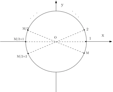
The structure of UCA is shown in Fig. 2.2. The total number ofM antenna sensors are uniformly located on a planar circle. The sensor elements are usually assumed isotropic. Therefore the element spacing can be obtained by the Sampling Theorem asd6 λ2. The

discrete-time signal model for a UCA is given by xm(i) = ej2πdλsinθcos(θ−γm) sin(φ)s(i) + nm(i), where s(i) is the zero-mean and complex narrowband signal source with power σ2

s, each of nm(i)is assumed to be zero-mean, spatially and temporally white Gaussian process and independent of s(i). γm = 2π(m ₋ 1)/N is the angle of the kth sensor measured counterclockwise from thexaxis. The azimuth angle θ _∈ [0,2π)is measured counterclockwise from the xaxis and the elevation angle φ ∈ [0, π)is measured down from thezaxis, which is perpendicular to the x-y plane [25].

θ τ (M−1)τ d x₁₍i₎ x₂₍i₎ x_M(i₎

Figure 2.1: Uniform Linear Array

2.3

Beamforming

When referring to beamforming, we usually consider the traditional or centralized beam-forming techniques, which are essentially signal processing techniques specified for using sensor arrays for directional signal transmission and reception. In traditional beamform-ing, we aim to combine the measurements from a uniformly configured antenna array to

y x 1 2 M/2 M/2+1 M/2+2 M O

Figure 2.2: Uniform Circular Array

maximize its gain in a specific direction, by phasing the array in a certain angle so that the desired signal(s) are enhanced and the undesired signal(s) or interferer(s) are attenuated or rejected. The most popular optimum beamformer is known as the MVDR (or Capon) beamformer [1], which is introduced in the following subsection.

2.3.1

MVDR Optimum Beamformer

The MVDR optimum beamformer aims to retrieve or extract a desired signal (signal of interest (SoI)) in a given direction and frequency with unit gain, while the weights are chosen to minimize the output power with a single linear constraint, which preserves the SoI and attenuates the interferences and noise [4]. In this case, the desired signal is not distorted [5] and the beamforming weight vectorw= [w1,· · · , wM]T is determined by

wM V DR=argmin w

E[|y|2_{] subject to w}H_{a= 1,}

(2.1) where y = wH_{x is the beamformer output acorresponds to the steering vector of the} SoI. By employing the Lagrange multiplier method, we need to minimize the Lagrangian function as described by

L(w, λ) = E[|y|2_{] +λ(w}H_{a−1) +λ}∗

(aHw−1)

where x is the array observation data and λ here is the Lagrange multiplier. Take the partial derivative of the above equation with respect towand equal it to zero, the weight vector is obtained as

wM V DR=−λR−1a. (2.3)

Substituting (2.3) into the linear constraint,λis obtained as λ =₋(aH_R−1_a)−1_.

(2.4) Combining (2.3) and (2.4) then we have the optimum MVDR weight as the following:

wM V DR =

R−1_a

aH_R−1_a. (2.5)

2.4

Adaptive Beamforming Algorithms

In adaptive beamforming, the statistics (e.g. the covariance matrix) are usually unknown and may change over time and need to be estimated from the available data [1, 4]. There are several approaches to learning the unknown statistics. One approach is to estimate the covariance matrix of the antenna observation data (e.g. implemented with Sampled Matrix Inversion (SMI) [1], which results in a SMI beamformer) [1]. Another approach is based on an optimization problem and employs conventional adaptive algorithms (e.g. Stochastic Gradient (SG) and Conjugate Gradient (CG) [21, 23, 24]) to realize the adap-tation of beamforming weights, which usually requires a low compuadap-tational complexity but converges slower than the SMI beamformer [1].

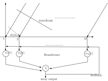
Fig. 2.3 describes the systematic diagram of an adaptive beamformer. Different from the optimum beamformer, the covariance matrix Rˆ is unknown and needs to be esti-mated in order to obtain the beamformer weights. One typical approach is to use the SMI method. In SMI, the covariance matrix is computed from the array observation data and referred to the Sampled Covariance Matrix (SCM) described by

ˆ R= 1 K K X k=1 x(k)xH(k), (2.6)

and its weight vector is computed as

wSM I =

ˆ R−1_a

θ(DoA) wavefront 1 2 M w₁(i) w 2(i) wM(i) P Beamformer array output feedback

Figure 2.3:Adaptive Beamformer

However, in real applications, the SMI approach will usually include a diagonal loading (DL) term (i.e. σ2_I

M, whereσ2is a constant and IM is an identity matrix of sizeM) [1]. Therefore, (2.6) is reformulated as ˆ R= 1 K K X k=1 x(k)xH_{(k) +σ}2_I M. (2.8)

The DL technique is an attractive modification to SMI beamformers because of its sim-plicity and potential performance improvement especially in a strong interference level situation. Even for a fixed DL, the loading level σ2 _{needs to be appropriately selected,}

which can be done by evaluating the signal and interference levels [1].

2.4.1

MVDR-LMS Adaptive Algorithm

The least mean squares (LMS) adaptive algorithm belongs to the class of stochastic gradi-ent (SG) methods. In this case, we consider deriving the LMS algorithm directly from the MVDR beamformer using the SG approach. To satisfy the MVDR beamforming criterion we have the following optimization problem:

minimize w(i) w

H_(i)R(i)w(i)

subject to wH(i)a= 1,

whereidenotes the time instant. Applying the SG recursion on its Lagrangian function [1], we have

w(i+ 1) =w(i)−µ∇L(w(i), λ) = w(i)−µ(x(i)y∗(i) +λa), (2.10) whereµis the step size,λis the Lagrange multiplier and_∇denotes the gradient operator. Substituting (2.10) into the constraint of (2.9), we have

(wH_{(i)−µ(x(i)y}∗_{(i) +λa))}H_{a= 1. (2.11)} Solving equation (2.11), we can obtain the Lagrange multiplierλ:

λ= −a

H_x(i)y∗_(i)

aH_a . (2.12)

Substitutingλback into (2.10) and simplifying the result, the beamforming weight adap-tation of MVDR-LMS algorithm is derived as

w(i+ 1) =w(i)−µy∗(i)(IM +

aaH

aH_a)x(i). (2.13)

2.4.2

MVDR-RLS Adaptive Algorithm

For the recursive least squares (RLS) algorithm, the optimization problem is defined as minimize y(i) = i X l=1 µi−l|y(l)|2 subject to wH(i)a= 1, (2.14)

whereiis the current time index,µis the forgetting factor andy(l) =wH_{(i)x(l). Again} by using the method of Lagrange multipliers, a Lagrangian cost function_Lis introduced

L=

i X

l=1

µi−lwH(i)x(l)xH(l)w(i) +λ(wH(i)a₋1) +λ∗(aHw(i)₋1). (2.15) Taking the partial derivative of (2.15) with respect tow(i)and equating the term to zero, we obtain w(i) = Φ −1_(i)a aH_Φ−1_(i)a = Λ(i)Φ −1_{(i)a, (2.16)} whereΦ(i) = Pi l=1

µi−l_x(l)xH_{(l)is the exponentially weighted sampled covariance matrix} andΛ(i) = (aH_Φ−1_(i)a)−1_{. To realize the recursion,Φ(i)is expressed as}

By using the Matrix Inversion Lemma for (2.17), we have the following

Φ−1_{(i) =Φ}−1_(i−1)− µ

2_Φ−1_(i−1)x(i)xH_(i)Φ−1_(i−1)

1 +µ−1_xH_(i)Φ−1_(i−1)x(i) . (2.18)

Let us define the following matrix quantities

P(i) = Φ−1_{(i) (2.19)}

and

g(i) = µ

−1_P(i−1)x(i)

1 +µ−1_xH_{(i)P(i−1)x(i)}, (2.20) whereg(i)is the gain vector, then (2.18) can be reexpressed as

P(i) =µ−1_{P(i−1)−µ}−1_g(i)xH_{(i)P(i−1). (2.21)} Multiplying both sides byx(i)and simplifying the terms, we have

g(i) = P(i)x(i) =Φ−1(i)x(i). (2.22) The weight vector is computed as

w(i) =Λ(i)P(i)a. (2.23)

After substituting (2.21) into (2.23), we then have the weight update equation as

w(i) = Λ(i)

µΛ(i−1)(I−g(i)x

H_{(i))w(i−1), (2.24)} which completes the MVDR-RLS adaptive algorithm [1].

2.4.3

MVDR-CG Adaptive Algorithm

We have already introduced the LMS and RLS algorithms under the MVDR criterion for adaptive beamforming. In fact, LMS has the advantage of simplicity but can not achieve good convergence performance as compared to RLS; while RLS demands a higher com-putational cost even though it has a high performance in convergence speed. In this sub-section, we review the CG adaptive algorithm which efficiently overcomes the disadvan-tages in LMS and RLS algorithms. Based on the linear constrained minimum variance (LCMV) criterion [1, 4], we start from the following optimization problem:

v=argmin v

where v _∈ CM×1 is the CG-based weight vector. A convex cost function J(v) can be described by [21, 23, 24] J(v) = 1 2v H_Rv − Re_{aHv_}. (2.26)

where_Re_{._} denotes the real part. The cost function is constructed in a quadratic form so that its gradient in terms of vdescribes the deviation of afrom Rv[21]. By taking the gradient of (2.26) with respect to v, equating it to a null vector and rearranging the expression we have

v=R−1_a.

(2.27) In order to derive the algorithm, we need to designate the snapshot indexiand the iteration indexkwhich is iteratively executed within each snapshot. Similar to the RLS algorithm, the data covariance matrix is estimated in a recursive fashion as:

ˆ

R(i) = λR(ˆ i₋1) +x(i)xH(i), (2.28) whereλis the forgetting factor, which is close to, but smaller than1. Taking the gradient of (2.26) with respect tovk(i)and choosing its negative direction, we obtain the negative gradient:

gk(i) = a−R(ˆ i)vk(i). (2.29) The definition for the CG-based weight vector is given by [21, 23, 24]

vk(i) = vk−1(i) +αk(i)pk(i), (2.30) where αk(i) is obtained by substituting (2.30) into (2.26) and taking the gradient with respect toαk(i), which gives

αk(i) = g H k (i)pk(i) pH k(i) ˆR(i)pk(i) , (2.31)

and the direction vectorpk(i)is updated by [21, 23, 24]

pk(i+ 1) =gk(i) +βk(i)pk(i), (2.32) whereβk(i)is given by [21, 23, 24] βk(i) = g H k (i)gk(i) gH k−1(i)gk−1(i) . (2.33)

AfterK iterations, the CG adaptive beamformer weight vector can be computed as

w(i) = vK(i) aH_v

K(i)

. (2.34)

Note that at the beginning of the next snapshot,gk(i+ 1)andpk(i+ 1)must be reset to

2.5

Robust Adaptive Beamforming

In this section, an explanation why RAB techniques are important for handling steering vector uncertainties and models for steering vector mismatch are provided. Furthermore, the most recent developed RAB algorithms are introduced and discussed.

2.5.1

Steering Vector Mismatch

When adaptive beamforming algorithms are applied to practical problems, the signal-to-interference-plus-noise ratio (SINR) performance may degrade when the data sample size is small and the convergence rate may reduce as the desired signal is presented in the training data [7]. Most importantly, the SINR performance of adaptive beamformers can suffer significant degradation because the underlying assumptions on the environment, signal sources or sensor array are usually non-ideal. This leads to a mismatch in the steering vector. To overcome the problem of steering vector mismatch, RAB techniques become a popular research area and various RAB algorithms have been developed.

In practical applications, different categories of steering vector mismatch include look direction and signal pointing errors, imperfect calibration and distorted antenna shape, manifold mismodeling due to source wavefront distortions, near-far field problem, signal fading and local scattering [7, 10].

Desired signal look direction mismatch is the simplest case for either modeling or handling. In this mismatch model, there exists an error for the DoA of the desired source signal (in some cases we also consider the interference signals). The error can be ei-ther a constant degree deviation or described by its statistical properties (e.g. uniform distribution within a certain range [14, 15]).

Near-far field mismatch is essentially caused by the spatial signature of the desired signal, which is assumed to be located in the near field of the antenna array, so that neither the array geometry nor the distance between the geometry center of the array and the signal source is negligible. In the case of ULA, the source is assumed to be located

on the line drawn from this geometrical center point in the normal direction to the array aperture, which is determined by the signal wavelengthλand the number of sensors M. The choice for the distance must be compatible with the array geometry parameters and also depends onM andλ[7].

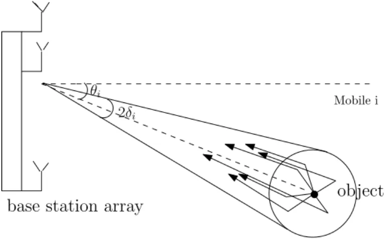
In the local scattering mismatch case as shown in Fig. 2.4 [9], we consider the source signal distributed (or scattered) due to the multipath scattering effect caused by the pres-ence of local scatterers [15]. This problem can be divided into two categories in terms of the signal signatures, called the coherent local scattering and incoherent local scattering.

object base station array

θi 2δi

Mobile i

Figure 2.4:Local Scattering Effect of Detecting a Moving Object from a Base Station Array

In coherent local scattering [7], the source signal is assumed to have time-invariant signature and the corresponding steering vector is modeled as

a=p+

L X

k=1

ejϕk_{b(θk), (2.35)}

where p corresponds to the direct path while b(θk)(k = 1,_{· · ·} , L) corresponds to the scattered paths. The anglesθk(k = 1,· · · , L)are randomly and independently drawn in each simulation run from a uniform generator with mean10◦ _{and standard deviation 2}◦_.

The anglesϕk(k = 1,_{· · ·}, L) are independently and uniformly taken from the interval

[0,2π]in each simulation run. Notice thatθk andϕk change from trials while remaining constant over snapshots [7].

signature and the corresponding steering vector is modeled by a(i) = s0(i)p+ L X k=1 sk(i)b(θk), (2.36) where sk(i)(k = 0,_{· · ·} , L)are i.i.d zero mean complex Gaussian random variables in-dependently drawn from a random generator. The angles θk(k = 0,· · · , L)are drawn independently in each simulation run from a uniform generator with fixed mean value and standard deviation. This time,sk(i)changes both from run to run and from snapshot to snapshot [7, 15].

2.5.2

Existing RAB Algorithms

In this subsection, we focus on the recently reported RAB algorithms. In [10], RAB design principles based on MVDR criterion have been discussed and summarized. These principles basically include: the generalized sidelobe canceller, diagonal loading [8, 9], eigenspace projection [18], worst-case optimization [7, 19] and steering vector estimation with presumed prior knowledge [11, 12].

The robust Capon beamformer (RCB) as discussed in [8] utilizes a diagonal loading method in which the loading factor is calculated based on a presumed uncertainty set for the SoI. It firstly started from an estimate of the desired signal power which is given by

˜

σ2 ₌ 1

aH_R−1_a, (2.37)

whereais the mismatched steering vector andRis the data covariance matrix. Further-more, the RCB approach leads to the optimization problem given by

min a a H_R−1_a subject to (a−a)¯ HC−1_(a−a)¯ 61, (2.38)

where botha¯andC−1_{are given. In the algorithm steps, an eigendecomposition technique}

and Newton’s method are required to deliver an estimate of the loading factor λ, which further helps with the estimation of the desired signal power σ˜2_{. This method has a}

Several of the most well-known online optimization programming based RAB ap-proaches include the worst-case optimization method [7], the sequential quadratic pro-gramme (SQP) method [12] and the method in [11], all of which aim to solve online optimization programmes (i.e. second order cone programme (SOCP) and semi-definite programme (SDP)) with presumed prior knowledge so that to obtain an estimate for the desired signal steering vector. The worst-case optimization method and [11] use the same uncertainty constraint for the steering vector mismatch as in the RCB method. How-ever, the SQP method uses a presumed steering vector that belongs to an uncertainty set A,{p+e,_ke_k6_}wherepis the presumed steering vector,eis the mismatch andis a known constant to restrict the uncertainty range. The presumed steering vectorpis then iteratively updated by adding the orthogonal part of the erroreand by enforcing that the updated version ofporthogonal to a subspace matrixP⊥

p, which is also orthogonal to the actual steering vectorp+e. This process can be expressed as an optimization programme described by min e (p+e) H_Rˆ−1 (p+e) subject to pHe= 0,P⊥_p(p+e) =0 (p+e)HC(p¯ +e)6pHCp¯ , (2.39)

whereRˆ is the SCM andC¯ =R

¯

θ

p(θ)pH_{(θ)dθ, whereθ}¯_{is the complement ofθ, which is} the angular sector in which the desired signal is assumed to be located,p(θ)is the steering vector associated with a particular directionθ, [11, 12, 14]. However, because of the very high computational cost (at least _O(M3.5_{)) for the online optimization programmes, the}

methods of [7,11,12] lack computation efficiency. Additionally, the direct implementation of SCM in both the optimization objective function and computation for the weight may reduce the accuracy and final SINR performance.

Some recent design approaches have considered combining different design principles together to improve RAB performance. In the algorithms of [14, 15], the data covariance matrix and the desired signal steering vector are separately and sequentially estimated. In both of these algorithms, the steering vector is estimated using the SQP method. However, the data covariance matrix in [14] is estimated by a linear shrinkage model expressed as

˜

R= ˆβRˆ + ˆαI, (2.40)

whereRˆ is the SCM,βˆandαˆare positive shrinkage parameters which are derived by min-imizing the mean squared error (MSE)MSE( ˜R) = E[kR˜ −Rk2], whereRis the actual

covariance variance rather than the SCM [14]. Essentially this shrinkage method belongs to the class of diagonal loading approaches with the loading factorα/ˆ βˆcomputable and adaptable. The algorithm in [15] approaches the covariance matrix estimation in a totally different way, which directly estimates the interference-plus-noise covariance(INC) ma-trix R˜i+n based on a INC matrix reconstruction method. It employs the Capon spatial spectrum estimator

ˆ

P(θ) = 1

dH_{(θ) ˆR}−1_d(θ), (2.41)

whereθcan be any possible angle,d(θ)is the steering vector associated with angleθand

ˆ

Ris the SCM. Furthermore, it is used for the INC matrix reconstruction as

˜ Ri+n = Z ¯ θ ˆ P(θ)d(θ)dH(θ)d(θ). (2.42)

The outstanding performance of [15] can be extremely close to the optimum SINR. How-ever, it has high potential computational cost when the number of sample points taken within the angular sectorθ¯is large.

The common point of all the above algorithms introduced is the difficulty of estimating the steering vector in a computationally efficient way. Efforts have been made to avoid high complexity especially with online optimization programmes and an attractive algo-rithm named low-complexity mismatch estimation (LOCME) has been developed in [13]. LOCME aims to estimate the steering vector mismatch with a cost of_O(M3_{)and does not}

require any optimization programme or additional information from the steering vector. It describes the estimation of the array steering vector as the projection onto a prede-fined subspace of the correlation between the beamforming output signal and the array observation vector as [13]

ˆ

a=√M Pd

kPd_k, (2.43)

wherePis the eigensubspace projection matrix which can be obtained if the angular range in which the steering vector is located is known anddis cross-correlation vector between the array observation dataxand the beamformer outputy, which is computed directly by

2.6

Distributed Beamforming

Distributed beamforming has been widely investigated in wireless communications and array processing in recent years [66–68]. It is key for situations in which the channels be-tween the sources and the destination have poor quality so that devices cannot communi-cate directly and the destination relies on relays that receive and forward the signals [67]. Other advantages of distributed beamforming include the ability to significantly increase system power gain and save energy [66]. This section discusses the concepts and prin-ciples of distributed beamforming as well as the typical optimization criteria used. The concept and principles of relay selection and robust distributed beamforming are also pre-sented and discussed.

2.6.1

Distributed Beamforming and Wireless Relay Networks

Distributed beamforming can be modelled as a relay network in which we consider a sin-gle or multiple (K) signal sources at the base station, a set of (M) distributed relays, each of which consists of only one sensor or antenna, and a destination. It is assumed that the quality of the channels between the signal sources and the destination is very poor so that direct communications is not possible. TheM relays receive information transmitted by the signal sources and then retransmit to the destination as a beamforming procedure, in which a simple two-step amplify-and-forward (AF) protocol or decode-and-forward (DF) protocol can be applied for cooperative communications. In an AF protocol, the relay nodes send out amplified and phased versions of their received signals, which re-quires much less delays and relay power consumptions. In a DF protocol, the relay nodes operate as a black box that decode the received signal and re-encode them before trans-mitting, which ensures higher security but is less efficient in terms of delay and energy consumption. There are other protocols like compress-and-forward (CF) which involves quantization procedures and is not efficient in many situations, in CF, the relays quan-tize the received signal in one block and transmits the encoded version of the quanquan-tized received signal in the following block, which requires very high complexity if the quanti-zation level is high or many blocks are used.

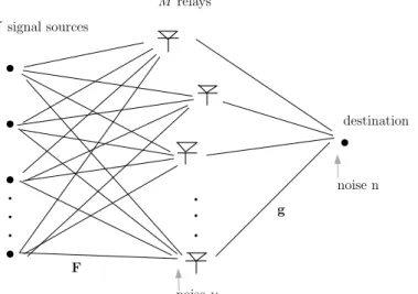
The relay network system can be modelled as shown in Fig. 2.5, assuming that an AF protocol is considered. Ksignal sources Mrelays destination F g noiseν noise n

Figure 2.5:System Model of Relay Network

In the first step, the sources transmit the signals to the relays as

x=Fs+ν, (2.44)

wheres = [s1, s2,· · · , sK] ∈ C1×K are signal sources with zero mean, [.]T denotes the

matrix transpose operator,sk = √Pks, E[_|s_|2_{] = 1, Pk is the transmit power of thekth}

signal source, k = 1,2,_{· · ·} , K, sis the information symbol. Without loss of generality we can assume s1 as the desired signal while the others are treated as interferers. F =

[f1,f2,· · · ,fK] ∈CM×K is the channel matrix between the signal sources and the relays, fk = [f1,k, f2,k,· · ·, fM,k]T ∈CM×1,fm,kdenotes the channel between themth relay and the kth source (m = 1,2,· · · , M, k = 1,2,· · · , K). ν = [ν1, ν2,· · · , νM]T ∈ CM×1

is the complex Gaussian noise vector at the relays and σ2

ν is the noise variance at each relay (νm˜CN(0, σν2)), whereCN(.)refers to complex Gaussian distribution. The vector

x∈CM×1represents the received data at the relays. In the second step, the relays transmit y_∈CM×1 which is an amplified and phase-steered version ofx, which can be written as

y=Wx, (2.45)

whereW= diag[w1, w2,· · · , wM]∈CM×M is a diagonal matrix whose diagonal entries

denote the beamforming weights. The signal received at the destination is given by

where z is a scalar, g = [g1, g2,· · · , gM]T ∈ CM×1 is the complex Gaussian channel

vector between the relays and the destination, n (n ˜ _CN(0, σ2

n), and we assume that σ2

n=σν2) is the noise at the destination andzis the received signal at the destination. Note that both F and g are modeled as Rayleigh distributed (i.e., both the real and imaginary coefficients of the channel parameters have Gaussian distribution). Using the Rayleigh distribution for the channels, we also consider distance based large-scale chan-nel propagation effects that include distance-based fading (or path loss) and shadowing. Distance-based fading represents how a signal is attenuated as a function of the distance and can be highly affected by the environment [69, 70]. An exponential based path loss model can be described by

γ =

√ L √

dρ, (2.47)

whereγ is the distance based path loss, Lis the known path loss at the destination, dis the distance of interest relative to the destination andρ is the path loss exponent, which can vary due to different environments and is typically set within 2to5[69, 70], with a lower value representing a clear and uncluttered environment which has a slow attenuation and a higher value describing a cluttered and highly attenuating environment. Shadow fading describes the phenomenon where objects can obstruct the propagation of the signal attenuating the signal further, and can be modeled as a random variable with probability distribution given by [69, 70]

β = 10(σsN₁₀(0,1))_,

(2.48) whereβ is the shadowing parameter,_N(0,1)means the Gaussian distribution with zero mean and unit variance,σs is the shadowing spread in dB. The shadowing spread reflects the severity of the attenuation caused by shadowing, and is typically given between0dB to9dB [69, 70]. The channels modeled with both path-loss and shadowing are described by

F=γβF0, (2.49)

g =γβg0, (2.50)

whereF0andg0denote the Rayleigh distributed channels without path-loss and

2.6.2

Optimization Criteria for Distributed Beamforming

Constraints are usually applied to relay systems in order to achieve desired objectives with environmental or self restrictions, which basically can be described as a single op-timization problem. According to the literature, there are three different categories of optimization problems for relay systems. The first one involves the minimization of the total transmit power of the relays subject to constraints on the quality of service (QoS), which is usually referred to the system output SNR or SINR in distributed beamforming systems. In this scenario, the optimization problem can be expressed as

min

w PT

subject to SNR(or SINR) _≥γ,

(2.51)

wherewis the beamforming weight vector,PT is the total transmit power, γ(γ > 0)is a predefined constant indicating the minimum required output SNR or SINR. It minimizes overall transmit power while ensuring the QoS is satisfied at the destination.

In the second scenario, the optimization problem is described as max

w SNR(or SINR)

subject to PT _≤PT,max,

(2.52)

which maximizes the output SNR or SINR while ensuring the total transmit power PT does not exceed the threshold or the maximum allowable total transmit powerPT,max.

In the third scenario, we have the following optimization problem: max

w SN R(or SIN R)

subject to Pm ≤PT,max for m= 1,2,· · · , M,

(2.53)

where Pm,max is the maximum allowable transmit power of the mth relay, from which each of the individual relay is constrained with a power limit. It should be emphasized that here we haveM constraints in total instead of a single one.

2.6.3

Centralized and Cooperative Relay Networks with an MMSE

Consensus Approach

For a centralized and cooperative relay network, we can always consider a minimum mean squared error (MMSE) consensus approach [71]. Assuming there are no interferers, then we definesˆm =φmxmand φm=arg min φm E[|s1−φmxm|2] = f∗ mP1 |fm_|2_P 1+σ2n , (2.54)

whereP1 is the desired signal power. Then we definesm˜ = _E[|sˆˆsmm|2] and the normalized relay weight wm˜ as wmφm

E[|sˆm|2], so that the total transmission power can be expressed as PM

m=1E[|w˜m˜sm|

2_{] =}PM

m=1|w˜m|

2_{. Therefore, the following optimization problem under}

a total power constraint is considered min ˜ wm M X m=1 κmE[|s1−gmw˜ms˜m|2] subject to M X m=1 |wm˜ _|2 ≤PT, (2.55)

whereκm >0and the solution of (2.55) is given by

˜ wm = g ∗ m λ/κm+|gm|2 r _γ m γm+ 1P1, (2.56)

whereλis the Langrange multiplier andγm =

|fm|2P1

Pn .

In order to solve the optimization problem in (2.55), an MMSE consensus approach is employed to enable local information exchange and cooperations among the relay nodes. Suppose information is shared by all relays and each relay has an individual auxiliary beamforming vector denoted as w˜m = [ ˜w1,m,w˜2,m,· · · ,wm,m˜ ]T, then (2.55) can be

re-formulated as follows: min {wm˜ } M X m=1 κmE[|s1−gmwm,m˜ ˜sm|2] subject to_||w˜m||2 ≤PT,w˜m =w, m = 1,2,· · · , M, (2.57)

where the second constraint is a consensus constraint to impose all weight vectors to be the same. Then a dual-decomposition method is applied to decompose (2.57) toM

sub-optimization problems for each relay node as follows: min ˜ wm M X m=1 κmE[_|s1−gmwm,m˜ sm˜ |2] subject to_||w˜m||2 ≤PT,w˜m =w. (2.58)

Suppose each relay node is connected to a subset of relay nodes denoted by _Mm. The second constraint in (2.58) can be replaced byw˜m = ˜wq, q ∈ Mm so that (2.58) can be reformulated as min ˜ wmE[|s1−gmwms˜m,1| 2_{] +λ} m(i)(||w˜m||2−PT) + X q∈Mm τ_m,qT ( ˜wm−w˜q), (2.59)

whereλm(i)andτm,q are Lagrange multipliers.The proposed algorithmic solution relies on the computation of the optimal weights and Lagrange multipliers at themth relay as

˜ wt,m =                    g∗ m λm(i)+|gm|2( g∗ m λ/κm+|gm|2 q γm γm+1P1− P q∈Mmτm,q;m 2 ), if t=m − P q∈Mmτm,q;t 2λm(i) , if t6=m (2.60)

where τm,q;t denotes the tth element of τm,q. The Lagrange multipliers are updated as follows

λm(i) = _|λm(i₋1) +µλ(_||w˜m||2−PT)|, (2.61) τm,q(i) = τm,q(i−1) +µτ(um−uq), (2.62) whereµλ andµτ are step sizes with small positive values, um = [|w1,m|,· · ·,|wM,m|]T

andiis the time index.

2.6.4

Generalized Relay Networks with SNR Maximization

Ap-proaches

As discussed before, there are two criteria used for maximizing the system output SNR -the total relay transmit power constraint and individual relay power constraint. With -the assumption that the second-order statistics of the CSI is perfectly known, [72] proved that

the system SNR maximization problem with a total relay transmit power constraint has a closed-form solution. It also showed that in the case of individual relay power constraints, the beamforming problem can be approximately written as a semidefinite programming (SDP) problem which can be efficiently solved using interior point methods.

The total relay transmit power can be rewritten as follows PT = M X m=1 E[|ym|2 ] = M X m=1 |wm|2 E[|xm|2 ] =wHDw, (2.63) wherew = [w1, w2,· · · , wM]T, D = P1diag([E[|f1|2], E[|f2|2],· · · , E[|fM|2]]) +PnI.

With the assumption that the relay noiseν1, ν2,· · · , νM, the destination noise n and the

channel coefficients g1, g2,· · · , gM are all independent from each other, the total noise power can be expressed by

Pz,n =E[ M X l,m=1 wmw_l∗gmgl∗]E[_|νm_|2_{] +E[} |n_|2_{] =w}H_{Qw+Pn, (2.64)} whereQ =PnE[ggH_{]. The power of the signal componentP}

1 can be expressed as Pz,1 =P1E[ M X l,m=1 wmw∗_lfmgmfl∗gl∗]E[|s|2_{] =w}H_{Rw, (2.65)} where R = P1E[(f g)(f g)H]. Therefore, the optimization problem for the SNR

maximization with total relay constraint can be expressed by [72]

max w wH_Rw wH_Qw+Pn subject towHDw≤PT. (2.66)

To solve the above optimization problem, the weight vector is rewritten as

w=√pD−1/2_{w˜, (2.67)}

wherew˜ satisfiesw˜H_{w˜ = 1. Then (2.66) can be rewritten as}

max {p,w˜} pw˜H_R˜_w˜ pw˜H_Q˜_{w˜ +Pn} subject to_||w˜||2 _{= 1, p≤PT,} (2.68)

where R˜ = D1/2_RD1/2 _{and Q}˜ _{= D}1/2_QD1/2_{. As the objective function in (2.68)}

maximized whenp=PT, hence (2.68) can be simplified as: max ˜ w PTw˜H_R˜w˜ PTw˜H_Q˜_{w˜ +Pn} subject to_||w˜||2 = 1, (2.69) or equivalently as max ˜ w PTw˜H_R˜_w˜ ˜ wH_{(PnI+PTQ) ˜}˜ _w subject to_||w˜_||2 _{= 1,} (2.70)

in which the objective function is maximized whenw˜ is chosen as the principal eigenvec-tor of(PnI+PTQ)˜ −1_R˜_{, which leads to the solution}

w=pPTD1/2P{(PnI+D1/2QD1/2)−1D1/2RD1/2}, (2.71) and the maximum achievable SNR is given by

SNRmax =PTλmax{(PnI+D1/2QD1/2)−1D1/2RD1/2}, (2.72) whereλmaxis the maximum eigenvalue.

Differently, we consider the following optimization problem for the scenario of indi-vidual relay power constraint as discussed in [67, 72]:

max w wH_Rw wH_Qw+Pn subject toDmm|wm|2 ≤Pm,form= 1,2,· · · , M, (2.73)

wherePmis the maximum allowable transmit power for themth relay andDmm refers to themth diagonal entry of matrixD. By definingX=wwH_{, (2.73) can be rewritten as}

max

X

tr(RX) tr(QX) +Pn subject toDmmXmm ≤Pm,form= 1,2,· · · , M,Rank(x) = 1,x0,

(2.74)

where Xmm refers to the mth diagonal entry of X. By using the idea of semidefinite relaxation and dropping the non-convex rank-one constraint, (2.75) can be reformulated as max {X,t} t subject totr(X(R−tQ))≥Pnt, Xmm ≤Pm/Dmm,form= 1,2,· · · , M,x0. (2.75)

It should be emphasized that for any value of t, the set of feasible X is convex. The problem (2.75) can be solved as a semidefinite programming (SDP) using interior points methods. The computational complexity and efficiency may vary based on the dynamics of solving an online convex programming with certain softwares.

2.6.5

Distributed Beamforming with Relay Selection

Distributed relays help by increasing system coverage and reducing power consumption. However, in most scenarios relays are either not ideally distributed in terms of locations or the channels involved with some of the relays have poor quality. Possible solutions can be categorized in two approaches. One is to adaptively adjust the power of each relay accord-ing to the qualities of its associated channels, known as adaptive power control or power allocation. Some power control methods based on channel magnitude and relative analy-sis has been studied in [73, 75]. An alternative solution is to use relay selection, which se-lects a number of relays according to a criterion of interest while discarding the remaining relays. In [77], several optimum single-relay selection schemes and a multi-relay selec-tion scheme using relay ordering based on maximizing the output SNR under individual relay power constraints are developed and discussed, but the beamforming weights are not optimized to enhance the SINR maximization. The work in [78] proposed a low-cost greedy search method for the uplink of cooperative direct sequence code-division multi-ple access systems, which approaches the performance of an exhaustive search. In [79], multi-relay selections algorithm have been developed to maximize the secondary receiver in a two-hop cognitive relay network.

From a general point of view, random relay selection is the simplest and most non-restrictive approach. With random relay selection, we choose the relays randomly. This can be done either by selecting a fixed number of random relays, or, with the number of selections to be decided randomly. We take a random decision for each relay that if it is to cooperate in the network with equal probability (i.e.,p(αm = 0) =p(αm = 1) = 0.5, where α = [α1, α2,· · · , αM]T ∈ {0,1}M×1 denotes the relay selection vector whose

element equals either 0 which means the corresponding relay is unselected, or1 which means the corresponding relay is selected). In case a fixed number of relays are required, the relay selection vector α is also randomly chosen, however, with a fixed number of

ones and zeros (number of ones=Mf ix, which is predefined).

Another popular approach is based on the exhaustive search method, in which we test every possible combination among all the relays, which means the change of status that each relay is chosen or not will contribute to a different possible combination. Also, if a minimum number of relays are required, then we can predefineMmin as the minimum required number of relays as an additional restriction. The exhaustive search method is expected to find out the best set of relays. However, the complexity can be extremely high depending on the total number of relays.

2.6.6

Robust Distributed Beamforming

In most practical scenarios, the channels that connect the signal sources and the relays may suffer quality degradation because of inevitable measurement, feedback delays, out-dated channel parameters, estimation and quantization errors in CSI [96–99] as well as propagation effects, which lead to an imperfect system CSI, which further results in unsat-isfactory system performance or even system failure. Because of the above reasons, RDB techniques are hence in demand to reduce or mitigate the channel errors or uncertainties and preserve the relay system performance. In the literature, very limited work has been done in the research area of RDB. Most of the existing techniques adopt a worst-case opti-mization design to constraint the system SNR and aim to minimize the total relay transmit power as in a convex optimization problem [98, 103, 104]. Similar approaches also start with the same optimization problem and then reformulate it so that it can be solved with using a convex semi-definite programme (SDP) relaxation method [94, 96, 97, 108]. The intriguing work in [96] models the channel errors on their covariance matrices as a type of matrix perturbation. However, all of these existing techniques designate to minimize the total relay transmit power with constraints on the QoS (e.g. SNRs, SINRs). If we denote the channel uncertainties or errors asE= [e1,· · · ,eK] ∈CM×K (If that only the

sources-to-destination channelFis considered for mismatch, whereasgis not affected), then we have

ˆ

fk=fk+ek, k = 1,2,· · · , K, (2.76) wherefk andˆfk are thekth true and mismatched channel components ofF, respectively.

we assume that ek falls in a hyper-spherical uncertainty set so that it satisfies the norm constraint_||ek|| ≤ k, wherek is a user-defined constant. The error uncertainly set can be hence written as

Ak={ζk|ζk =fk+ek,||ek|| ≤k}, k= 1,· · · , K. (2.77) Then the optimization problem that aims to minimize the total relay transmit power with a SNR contraint can be generally described by

min

w PT subject to SN R > η,

(2.78)

whereηis the minimum requirement for the system input SNR.

2.7

Summary

This chapter has firstly reviewed the background theories of sensor array processing and beamforming techniques. Then, introductions to the existing work in the literatures on the conventional adaptive beamforming algorithms and robust adaptive beamforming tech-niques have been presented. Lastly, the problem of distributed beamforming for wireless communication systems and the existing approaches and techniques have been discussed. This chapter is provided as a background support to the rest of the chapters where sig-nificant improvements and developments as well novel techniques are proposed. In the following chapters, we firstly introduce novel cost-efficient robust adaptive beamform-ing methods that based on recursive shrinkage methods, cross-correlation exploitations, subspace projections and low-rank techniques. Then, distributed beamforming and relay selection methods and robust distributed beamforming techniques are proposed.

Low-Complexity Shrinkage-Based

Mismatch Estimation (LOCSME)

Algorithms for Robust Adaptive

Beamforming

Contents

3.1 Introduction . . . 35 3.2 System Model and Problem Statement . . . 37 3.3 Batch LOCSME Algorithm . . . 38 3.4 Stochastic Gradient LOCSME Type Algorithm . . . 42 3.5 Conjugate Gradient LOCSME Type Algorithms . . . 45 3.6 Performance Analysis . . . 51 3.7 Simulations . . . 57 3.8 Summary . . . 62