Efficient tuning parameter selection by
cross-validated score in high dimensional models
Yoonsuh Jung
Abstract—As DNA microarray data contain relatively small sample size compared to the number of genes, high dimensional models are often employed. In high dimensional models, the selection of tuning parameter (or, penalty parameter) is often one of the crucial parts of the modeling. Cross-validation is one of the most common methods for the tuning parameter selection, which selects a parameter value with the smallest cross-validated score. However, selecting a single value as an ‘optimal’ value for the parameter can be very unstable due to the sampling variation since the sample sizes of microarray data are often small.
Our approach is to choose multiple candidates of tuning parameter first, then average the candidates with different weights depending on their performance. The additional step of estimating the weights and averaging the candidates rarely increase the computational cost, while it can considerably improve the traditional cross-validation. We show that the selected value from the suggested methods often lead to stable parameter selection as well as improved detection of significant genetic variables compared to the tradition cross-validation via real data and simulated data sets.
Keywords—Cross Validation, Parameter Averaging, Parameter Selection, Regularization Parameter Search
I. INTRODUCTION
D
NA microarray data provide measurements of the expression levels of thousands of genes with relatively small samples. Classification and regression models play an important role in constructing statistical models to analyze the microarray data. For this reason, numerous of statistical models have been developed to model microarray data [1]–[4]. As many regression and classification models for high dimensional data involve tuning parameters, selection of the parameter is a crucial part of modeling procedure. For example, as the array’s disease status is often binary, and sample size is smaller than the number of genes, a class of penalized logistic regressions is in good shape for modeling the microarray data. To select potentially important genes, works in [5]–[7] selected the penalty parameter by cross-validation (CV).In fact, the statistical software R packages frequently adopt cross-validation for selecting penalty parameters. [8] developed an R package ncvreg which can fit logistic regressions with LASSO [9] penalty. Cross-validation is embedded for selecting the penalty value in the package. Many other R packages for fitting penalized regression also employ cross-validation. A few examples are glmnet for implementing the works of [10] and [11],glmpathfor [12], andgenlassofor [13]. Although huge volume of penalized regression models have been developed recently, leave-one-out
Yoonsuh Jung, Lecturer, is with the Department of Statistic, University of Waikato, Hamilton, New Zealand. (e-mail: [email protected])
cross-validation (LOOCV) [14] and K-fold cross-validation (KCV) [15] are still widely used. This is due to the attractive property of the cross-validation, which does not assume any underlying distribution of the data.
Classification technique is another common statistical methods in analyzing microarray data. In classification, CV has been broadly conducted for the training and evaluation of classifiers. Again, most of the classifiers require to determine ‘optimal’ parameters. For example, [16], [17] applied support vector machine (SV M) and [18] utilized random forest to microarray data sets and used CV method for choosing ‘optimal’ parameters. [19], [20] involved CV in clustering methods for analyzing microarray data.
Among various CV methods [21], K-fold CV (KCV) is very popular, and is more efficient than LOOCV. When K is the same as sample size, it is equivalent to LOOCV. However, [22], [23] pointed out that CV is highly variable estimate of the error although it is unbiased. This fact motivates us to develop new CV methods which could reduce the variability significantly, while may allow slight bias. For this purpose, we recycle the cross validated errors (or, the prediction errors) that arise during the process of cross-validation. Cross validated errors have been used only for comparing candidates of models or parameter values. As more plausible models (or, parameter values) are likely to produce smaller prediction errors, the errors are used for the final judgement only. That is, current CV methods select a single parameter value with the smallest prediction error. However, due to variations in splitting the data set into K parts, the selected parameter value with the minimum prediction error (based on test data) is not necessarily the best value for the whole data. Furthermore, there exists random variation in the data set itself.
To reflect these variations, the proposed methods first select the candidates of parameter values which give relatively small prediction errors. Secondly, we average the candidate values with different weights in which the cross validated errors are used to estimate the weights. That is, we impose more weight on the parameter value with less prediction error among the candidate values. Then, due to the averaging, we can reduce the variance of the estimate of the tuning parameter. Improved selection of the tuning parameter may result in better estimation and variable selection in turn.
Section II describes the details of the form and implementation of the suggested method. We apply our methods to real data and simulated data in Section III and Section IV, respectively.
II. EFFICIENT CROSS-VALIDATION A. Efficient K-fold Cross-validation
Supposexiis vector ofp-dimensional observations andyi∈
{0,1} is a binary response for i = 1, . . . , n. In general, the standard logistic regression shows conditional class probability of y by
logP r(y= 1|x)
P r(y= 0|x) =β0+x 0
iβ. (1)
Then, the penalized logistic regression usually fits this model through penalized maximum likelihood. Letp(xi) =P r(yi=
1|xi). Then, the penalized log likelihood is
1 n n X i=1 {yilogp(yi) + (1−yi) log(1−p(yi))} −λP(β), (2)
whereP(β)is the penalty forβ, andλis a tuning parameter. Maximum likelihood type of approach can be used for the estimates ofβ. Then, the estimate ofλchosen byK-fold CV (KCV) procedure is represented as
ˆ
λKCV = arg minλ∈[0,λmax]
n X
i=1
I(yi6= ˆyi(λ)), (3)
whereyˆi(λ)is the predicted value for theith observation.
Now, the proposed methods first select M candidates of λ values, ˆλm, m = 1, . . . , M from KCV. Suppose δˆm =
Pn
i=1I(yi6= ˆyi(ˆλm))/nis the prediction error rate associated
with λˆm. To select the candidates, there should be a certain
criterion. For example, we may select λˆm which satisfies
maxm=1,...,Mδm≤c1·δmin, whereδmin= minm=1,...,Mδm
and 1≤c1 ≤cmax. That is, we consider ˆλm as a candidate
only when the corresponding prediction error rate is less than cmax times that of the minimum error rate.
Alternatively, we may use rankings of λˆms in terms of
prediction error rate to pick the candidates. For example, top 5, or top 10ˆλmvalues by the rankings of the prediction errors
can be considered as candidate values of the tuning parameter. Then, the final λ value selected by the suggested efficient K-fold CV (EKCV) is defined as following;
ˆ λEKCV = 1 M M X m=1 ˆ wmλˆm, (4) where wˆm = (1/δˆm)/(P M
m=11/δˆm) is the estimated weight
for λˆm. The estimate of the weights is designed to be large
when the prediction error rate is small, and is normalized to maintain its sum as one. Sometimes, we may find one or multiple δˆm values are zero when the predicted values are
all the same as the observed values. This can happen when prediction is an easy task. This causes infinite weight (since ˆ
δm= 0) and cannot estimate the weights. In practice, one can
replace it with a large weight such as twice of the maximum weight except for the infinite weight. Notice that KCV method is, in fact, a special case of EKCV withM=1 andδmin. From
the nature of averaging, λˆEKCV may maintain substantially
reduced variance when compared to λˆKCV.
In terms of computation, EKCV requires almost the same amount computing as KCV does. Splitting the data into K
folds and iterative training and validation are the common procedures for KCV and EKCV, which comprises majority of the computation. The additional computing is the calculation of the weights,wˆms, and finding the final value of (4), which
takes ignorable amount of time.
As the domain ofλ is a subset of real line,λ∈[0, λmax],
we cannot search all possible values. But, we can only search limited number of λs in practice. Thus, λ values on a grid, for example, equally spaced points on the grid, are what researchers can examine in practice. Of course, using finer grid will lead to more accurate estimate of the tuning parameter, but it increases computation. The amount of computation increases linearly as we increase the number of values to be searched on a grid. Note thatλˆEKCV in (4) is not necessarily one of
the values on the grid, which could have been found by KCV with finer grid. In this respect, the proposed method has certain effect of employing a finer grid without adding more points to the grid. Thus, it is possible to view the proposed method as computationally efficient method to a certain degree.
As KCV is broadly used beyond the penalized logistic regression models, we can use EKCV to the other procedures. Here is a general EKCV algorithm.
ALGORITHM 1
1) Fit a model usingK−1folds of the data (training data). 2) Evaluate the fitted model on the hold out data (test data). 3) Iterate step 1 and 2 forKtimes to have predicted values
for all observations.
4) Select candidates of models (or, parameters) based on cross validated score (or, prediction error).
5) Obtain a weighted average the candidates of models utilizing the cross validated score, which is a final model. Note that algorithm 1 can be used to select any tuning parameter. For example, we can apply the above procedure to select the scale parameter in the radial basis kernels of support vector machine (SV M) [24]. Currently, KCV is embedded in R packages forSV M such as e1071[25],kernlab [26], and ascrda [27]. We can replace KCV with the proposed EKCV for improving the tuning parameter selection, and this is indeed the case, which will be shown in Sections III and IV.
B. Efficient Cross-validation
The main concept of the suggested methods can be applied to different versions of cross-validation procedure. One of the popularly used cross-validation methods is to split the data into two parts randomly. Next, one part of the data is used for training models (training data), and the other for evaluation (test data). Then, the best model is selected based on the prediction error from the test data by comparing the prediction errors. Now, the efficient cross-validation of our suggestion can select candidates of models and form a ultimate model by calculating a weighted average. Again, we can use the reciprocals of the prediction errors as estimates of the weights. To build an general algorithm, we can modify the algorithm 1 by specifying K = 2, and removing step 3. As the modification is simple, we do not provide another formal algorithm for this type of two-fold cross-validation.
C. Comparison with Other Approaches
Model selection methods based on likelihood such as BIC [28] and AIC [42] are well-known criteria. However, [29] indicated that the original BIC does not work well for high dimensional models. [30] showed BIC is not consistent under linear model when both n and p increase, and suggested a modified version. But, [30]’s method still requires p < n, which does not hold for the case of penalized logistic regression models for fitting typical microarray data ofn < p. Later, [31] proposed extended BIC methods tailored to high dimensional models, and its form is given below.
EBICγ(s) =−2ln( ˆβ(s)) +ν(s) logn+ 2ν(s)γlogp, (5)
where βˆ(s) is the maximum likelihood estimator of β(s) given model s, andν(s)is the number of non-zero variables (or components) in s. When γ = 0, EBICγ is equivalent
to the original BIC. [31] performed extensive simulation studies under penalized logistic regression models with γ = 0,0.25,0.5,and 1. AsEBICγ is designed for regression, and
not for classification, we employ this for regression models to compare to the proposed methods.
III. REAL DATA ANALYSIS
We compare the performance of EKCV with KCV and EBICγ withγ= 0,0.25,0.5 and 1 on four DNA microarray
data sets that are publicly available. Both of the regression and classification models are investigated for this purpose. For the regression methods, we employ penalized logistic regression for binary response and penalized multinomial regression for more than two categorical response. For the forms of penalty, lasso-type [9] and ridge-type [32] of penalties are examined, that is, P(β) = Pp j=1|βj| and P p j=1β 2 j, respectively. R
package glmnetis used for the implementation.
For classification,SV Mwith radial basis kernel is adopted where the selection of scaling parameter is our main interest. We utilize R package kernlab for the implementation where bound-constraint SV M classification [33] is used by specifying type=“C-bsvc” in ksvm function. Here, the classification accuracy of SV M will be vary depending on the choice of the scale parameter.
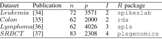
The summary of the four data sets are given in Table I where I stands for the number of categories in the response variable. The data sets are contained in the specified R packages.
TABLE I
SUMMARY AND SOURCE OF THE DATA SETS.
Dataset Publication n p I Rpackage
Leukemia [34] 72 3571 2 spikeslab
Colon [35] 62 2000 2 rda
Lymphoma[36] 62 4026 3 spls
SRBCT [37] 83 2308 4 plsgenomics
With the data sets in Table I, we choose the penalty or scale parameter (for SV M) using EKCV, KCV, andEBICγ
in (5). For EKCV, Algorithm 1 in Section II-A is applied to find the final value of the tuning parameter. As the results fromEBICγ withγ= 0,0.25,0.5and 1 are all identical, we
show the results only once. This is because the last term in RHS of (5) chances only slightly for four different γ values with the given data sets. ForKCV andEKCV, we try 300 different random splits, and mean of the prediction error rates and its standard error (in the parenthesis) are reported. We use K = 5 for all the implementations. The error rates (or, misclassification rates) are summarized in Table II. In the table, Lasso is logistic (for I = 2) or multinomial logistic regression (for I > 2) with lasso-type penalty. Similarly, Ridgeis with ridge-type penalty, and SV M is the described support vector machine. As there are no K random splits when EBIC in (5) is applied, there is no standard error of the error rate. In Table II, EKCV shows the lowest error rate
TABLE II
MEAN OF ERROR RATES(IN%)AND ITS STANDARD ERROR(IN PARENTHESES).
Leukemia Colon LymphomaSRBCT
Lasso KCV 0.009 (0.01) 1.575 (0.18) 0 (0) 0 (0) EKCV 0.014 (0.01) 1.086 (0.14) 0 (0) 0 (0) EBICγ 2.778 8.065 0 0.365 Ridge KCV 0 (0) 0.194 (0.04) 0 (0) 0 (0) EKCV 0 (0) 0.145 (0.04) 0 (0) 0 (0) EBICγ 0 4.84 0 0 SVM KCV 0.653 (0.04) 6.715 (0.09) 0 (0) 0 (0) EKCV 0 (0) 5.565 (0.05) 0 (0) 0 (0)
compared to other methods in most cases. In general, the error rates are low and SRBCT is the easiest to classify even if there are four categories in the response.Colondata set shows relatively higher error rate across different methods where the favorable performance EKCV is well appealed. In fact, we applied the penalized linear discriminant analysis [38], but the results are equal for KCV and EKCV across four data sets, thus not shown, although the selected penalty parameter values are different. From further investigation, we observed that the classification by penalized linear discriminant analysis is not sensitive to the value of chosen penalty parameter.
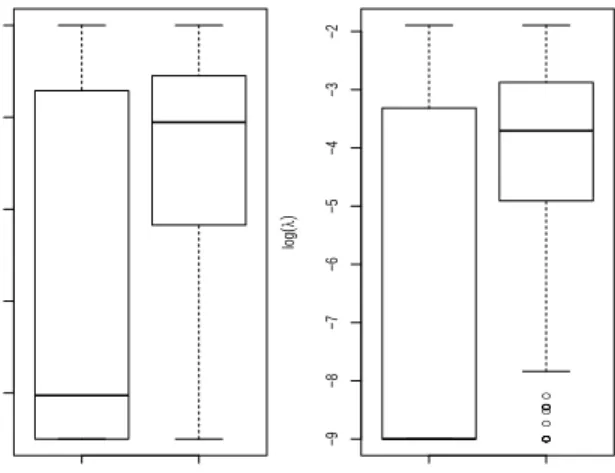
In Figure 1, we compare the distribution of selected parameter values by KCV and EKCV, that is, the distribution of ˆλKCV and λˆEKCV. We observe that the distributions of
the selected penalty parameter from EKCV show much less variability when compared to those from KCV in both of Colon and SRBCT data. The reduced variance is due to the averaging of multiple candidates.
Now, we examine another cross-validation study described in Section II-B. We split the data sets into training and test data. Half of the data sets are randomly selected and assigned as a training data set, while the other half are used as test data. We use the training data set for model construction only, and predict the value of response variable in the test data. This process is slightly different from Algorithm 1 as we do not get the predicted values for the whole response variable. However, settingK=2, and removing the step 3 in algorithm 1 will do the same process. AsEBICγ is needed to be applied to the
KCV EKCV −10 −8 −6 −4 −2 Colon log ( λ ) ● ● ● ● ● ● ● ● ● ● ● ● ● ● KCV EKCV −9 −8 −7 −6 −5 −4 −3 −2 SRBCT log ( λ )
Fig. 1. Distribution of selected parameter (log(λ)) by KCV and EKCV from ColonandSRBCT data set.
with KCV and EKCV. Again, we repeat the described process for 300 times and the mean error rates and its standard error is given in Table III.
TABLE III
MEAN OF ERROR RATES(IN%)AND ITS STANDARD ERROR(IN PARENTHESES)BYKCVANDEKCVFROM300 MONTECARLO DATA
SETS. TRAINING DATA SET CONTAIN1/2OF THE SAMPLES.
Leukemia Colon LymphomaSRBCT
Lasso KCV 0 (0) 0.290 (0.18) 0 (0) 0.103 (0.6) EKCV 0.009 (0.01) 0.097 (0.14) 0 (0) 0.095 (0.06) Ridge KCV 2.509 (0.52) 0 (0) 0 (0) 0.175 (0.05) EKCV 0.111 (0.11) 0 (0) 0 (0) 0.135 (0.04) SV M KCV 0.435 (0.06) 4.301 (0.46) 0 (0) 0.238 (0.07) EKCV 0 (0) 0.796 (0.10) 0 (0) 0 (0)
We can see the error rates from EKCV are smaller than those from KCV in most of the cases. However, we cannot compare the two methods when the error rates are all zero. This leads us to repeat the same experiments with smaller number of training sample size. For this reason, we assign only quarter of the data to the training data and three quarters to the test data. The results from this modified experiment are in Table IV.
In Table IV, the improved performance of Lasso and SV M by the suggested EKCV becomes more apparent, while the error rates from Ridgeare mostly zero. Especially, incorporating EKCV in SV M shows remarkably higher prediction accuracy for Colon data set compared to the accuracy of KCV.
IV. SIMULATION STUDIES
We consider 2000 genes with 400 samples for all of the simulations. To generate simulated microarray data set with binary response, we first generate gene expression data from multivariate normal distribution. That is, X ∼M V N(0,Σ), where 0is a zero vector of size pandΣ is pby pvariance
TABLE IV
MEAN OF ERROR RATES(IN%)AND ITS STANDARD ERROR(IN PARENTHESES)BYKCVANDEKCVFROM300 MONTECARLO DATA
SETS. TRAINING DATA SET CONTAIN1/4OF THE SAMPLES.
Leukemia Colon LymphomaSRBCT
Lasso KCV 0.031 (0.02) 0.906 (0.14) 0.156 (0.09) 0.047 (0.05) EKCV 0.019 (0.01) 0.529 (0.10) 0.014 (0.01) 0 (0) Ridge KCV 0 (0) 3.551 (0.45) 0 (0) 0 (0) EKCV 0 (0) 4.819 (0.60) 0 (0) 0 (0) SV M KCV 2.383 (0.51) 11.22 (0.76) 0 (0) 1.534 (0.55) EKCV 0 (0) 2.014 (0.11) 0 (0) 0 (0)
covariance matrix with p = 2000. The correlation between Xi and Xj are set to ρ|i−j| with ρ = 0.3. This correlation
structure mimics the situation where nearby genes are more correlated. The correlation will be attenuated as the distance between two variables increases. The response variable Y is randomly generated from Bernoulli(π(X)) where π(X) = (1 + exp(−f(X)))−1. We examine the following
response models of f(X).
Model 1 (M1).f(X) =Xβ. For the regression parameter β, we set, without loss of generality, the first 30 to be non-zero values and the other 1970 values to be zero. β = (0.5, ...,0.5,1, ...,1,1.5, ...,1.5,2, ...2,2.5, ...,2.5,0, ...,0)0. Thus, the first 30 variables with five different magnitudes are related to the response variable with different magnitude. Note that there are six identical values in each magnitude.
Model 2 (M2).f(X) = (Xβ)·(1 +Xγ). The value ofβ is the same as we have inM1. The first 30 elements ofγare randomly drawn from uniform distribution on (0,0.3), while the other 1970 elements are zero. This setting is designed to follow the situation when genes interact with each other.
Model 3 (M3).f(X)is the same asM2except that 3% of X (or, the first 12 rows of X) are tripled. This modification causes heavy tailed distribution of X deviated from the normality, which is often observed in gene expression data.
Once the data set is generated, we randomly split it into training data of sample size 300, and test data with the other 100 samples.
We first apply penalized logistic regression with lasso penalty (Lasso), adaptive lasso penalty [39] (Alasso), and ridge penalty (Ridge), and also apply the boundary constrained SV M (which we employed in the previous Section) to the training data set and select the penalty parameter ofλbased on the prediction error rates from the test data. This is the traditional cross-validation procedure (CV). Secondly, using the same method of Lasso,Alasso, Ridge, andSV M, we select the value ofλ based on the suggested efficient cross-validation (ECV). We repeat the described procedure for 300 times to reduce the undesirable effect of random variation arises from generating X and splitting the
data.
We compare CV and ECV in several aspects of (A). prediction accuracy, (B). estimation ofβ, and (C). detection of significant (non-zero) variables. We report prediction accuracy of CV and ECV only for SV M since (B) and (C) cannot be obtained viaSV M. Although there are interaction effects (caused by γ) in M2 and M3, we use the linear model and measure accuracy of estimation in terms of β. Thus, we will approximate the associations between the genes by the independent model (without interaction) for M2 and M3, and gauge their (approximated) estimation accuracy. This approximation by independent model is attractive as there are 2000 genes, and considering interaction terms among them will result in huge (about 2 million) number of variables, which we want to avoid here. But, there are some works ( [40] and references given in Section 3.3 of [41]) which efficiently detect the potential interactions.
Now, we describe the results under the above aspects of (A), (B), and (C).
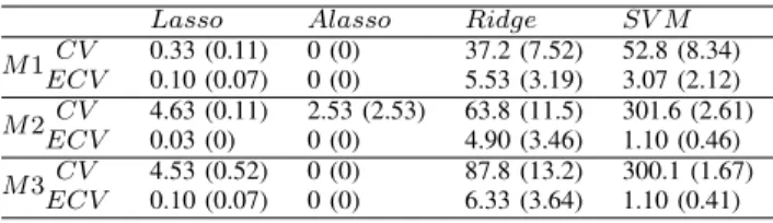
Aspect (A). We compare the prediction error rates by the two methods (CV and ECV). From 300 Monte Carlo data sets, the mean of the prediction error rates and its standard error is given in Table V.
TABLE V
MEAN OF PREDICTION ERROR RATES AND ITS STANDARD ERROR(IN PARENTHESES)FROM300 MONTECARLO DATA SETS. ALL VALUES ARE
MULTIPLIED BY103.
Lasso Alasso Ridge SV M M1CV 0.33 (0.11) 0 (0) 37.2 (7.52) 52.8 (8.34) ECV 0.10 (0.07) 0 (0) 5.53 (3.19) 3.07 (2.12) M2ECVCV 4.63 (0.11) 2.53 (2.53) 63.8 (11.5) 301.6 (2.61) 0.03 (0) 0 (0) 4.90 (3.46) 1.10 (0.46) M3CV 4.53 (0.52) 0 (0) 87.8 (13.2) 300.1 (1.67) ECV 0.10 (0.07) 0 (0) 6.33 (3.64) 1.10 (0.41)
The error rates from both the methods are very low. Especially, the prediction errors using adaptive lasso penalty are close to zero. We can see that there are significant improvements in terms of prediction accuracy by switching fromCV toECV in case ofRidgeandSV M. The improved performance of SV M by ECV is somewhat surprising because the additional step in ECV is just simple weighted averaging of the candidate values of the parameter. With the minimal additional computation, the prediction error ofSV M is reduced significantly.
Aspect (B). Now, to compare the performance of estimating β, we calculate the empirical mean squared error (M SE) by
S−1
S X
s=1
kβˆ(s)−βk2, (6) where βˆ(s) is the vector of estimated value of β from sth
simulated data set. Here, S = 300. Further, we decompose the empirical M SE into the variance and squared bias. The details form of empirical variance (V ar) is
S−1 S X s=1 kβˆ(s)−S−1 S X s=1 ˆ β(s)k2, (7)
and the empirical squared bias (Bias2) is
S−1 S X s=1 kS−1 S X s=1 ˆ β(s)−βk2. (8) V ar, andBias2 fromCV andECV are presented in Table
VI. Although the two methods yield similar M SE values, switching from CV to ECV shows that the amount of reduction in variance is greater than the increased squared bias in most cases.
TABLE VI
EMPIRICAL VARIANCE(V ar)AND SQUARED BIAS(Bias2)OFLasso, Alasso,ANDRidgeAS DEFINED IN(7),AND(8)FROM300 MONTE
CARLO DATA SETS. ALL VALUES ARE MULTIPLIED BY103.
Lasso Alasso Ridge
V ar Bias2 V ar Bias2 V ar Bias2 M1CV 0.709 29.84 8.731 10.24 4.786 31.50 ECV 0.484 30.04 5.035 13.44 2.513 34.09 M2CV 1.391 39.29 12.11 34.83 2.902 38.55 ECV 1.026 39.05 8.249 35.71 1.371 39.26 M3CV 1.545 39.30 12.22 35.10 2.994 38.57 ECV 1.139 39.11 8.448 35.84 1.482 39.25
Due to the averaging effect, we expect to see some reduction in the variance. But, it is interesting to see that both the variance and the squared bias from Lasso estimates are decreased byECV. The results in Alasso and Ridgeshow typical pattern of bias-variance tradeoff. Except for the results of Ridge under M1, all the M SE values from ECV are smaller than those fromCV.
Aspect (C). Now, we compare the identification of truly non-zero regression parameters under Lasso and Alasso. Note that the first 30 elements in β are non-zero in the simulation settings. We count the number of correct detections of non-zero elements and also record the false negative identification by CV and ECV. The results from Lasso is summarized in Table VII. We see that the suggested method
TABLE VII
MEAN NUMBER OF TRUE DETECTION(P+)AND MEAN NUMBER OF FALSE NEGATIVE(N−)AND THE STANDARD ERRORS(IN PARENTHESIS)FROM
Lasso. Lasso Alasso P+ N− P+ N− M1 ECVCV 21.5 (0.13) 8.37 (0.13) 22.5 (0.10) 7.53 (0.10) 21.9 (0.11) 8.01 (0.12) 22.4 (0.10) 7.58 (0.10) M2 CV 6.66 (0.14) 23.3 (0.14) 8.16 (0.12) 21.84 (0.12) ECV 7.74 (0.12) 22.3 (0.12) 8.14 (0.12) 21.86 (0.12) M3 ECVCV 6.27 (0.13) 23.73 (0.13) 7.78 (0.12) 22.22 (0.12) 7.45 (0.12) 22.55 (0.12) 7.69 (0.12) 22.30 (0.12)
detects slightly more significant variables and shows reduced number of false negative identifications forLasso, but cannot see any difference between CV and ECV for Alasso. As Ridge method cannot have exactly zero estimate, the results are not shown here.
V. CONCLUSION
In this work, we set our main focus on improving the model selection (or, variable selection) by averaging the candidates
of parameters using different weights. To estimate the weights, prediction error produced by cross-validation is employed. We impose higher weight to the parameter value with lower predicted error. We use the reciprocal value of the error rate as a specific form of the estimated weights. However, there could be other estimates of the weights. One who wish to use stabler estimated weights may add some positive constant to the error rates, and then use the reciprocal value of the inflated error rates. Alternatively, we can shrink the estimated individual weights (wˆi) to the average weight (P
n
i=1wˆi/n).
Since there are random variation in the sample, this may work well especially when the sample size and/or number of candidate models is small.
Researchers in biostatistics and bioinformatics are often interested not only in the accurate classification but also in detecting important genetic variables from the microarray data set. We see some potentials of the suggested methods towards these aims via the real data analyses and simulation studies. As the suggested methods can be readily incorporated to the penalized regression type of model, we mainly applied the suggested methods to analyze the microarray data. But, its application to other types of modeling procedures sounds plausible. For example, it maybe worthwhile to investigate the area of high dimensional linear models with the continuous response variable.
REFERENCES
[1] J. Zhu and T. Hastie, “Classification of gene microarrays by penalized logistic regression,”Biostatistics, vol. 5, no. 3, pp. 427 – 443, 2004. [2] L. Shen and E. C. Tan, “Dimension reduction-based penalized logistic
regression for cancer classification using microarray data,”IEEE/ACM Transactions on Computational Biology and Bioinformatics, vol. 2, no. 2, pp. 166 – 175, 2005.
[3] C. Li and H. Li, “Network-constrained regularization and variable selection for analysis of genomic data,”Bioinformatics, vol. 24, no. 9, pp. 1175 – 1182, 2008.
[4] W. Pan, B. Xie, and X. Shen, “Incorporating predictor network in penalized regression with application to microarray data,”Biometrics, vol. 66, pp. 474 – 484, 2010.
[5] G. Fort and S. Lambert-Lacroix, “Classification using partial least squares with penalized logistic regression,” Bioinformatics, vol. 21, no. 7, pp. 1104 – 1111, 2005.
[6] G. C. Cawley and N. L. C. Talbot, “Gene selection in cancer classification using sparse logistic regression with bayesian regularization,” Bioinformatics, vol. 22, no. 19, pp. 2348 – 2355, 2006.
[7] L. Waldron, M. Pintilie, M.-S. Tsao, F. A. Shepherd, C. Huttenhower, and I. Jurisica, “Optimized application of penalized regression methods to diverse genomic data,”Bioinformatics, vol. 27, no. 24, pp. 3399 – 3406, 2011.
[8] P. Breheny and J. Huang, “Coordinate descent algorithms for nonconvex penalized regression, with applications to biological feature selection,”
The Annals of Applied Statistics, vol. 5, no. 457, pp. 232 – 253, 2011. [9] R. Tibshirani, “Regression shrinkage and selection via the lasso,”
Journal of the Royal Statistical Society. Series B (Methodological), vol. 58, no. 1, pp. 267 – 288, 1996.
[10] J. Friedman, T. Hastie, and R. Tibshirani, “Regularization paths for generalized linear models via coordinate descent,”Journal of Statistical Software, vol. 33, no. 1, pp. 1 – 22, 2008. [Online]. Available: http://www.jstatsoft.org/v33/i01/
[11] N. Simon, J. Friedman, T. Hastie, and R. Tibshirani, “Regularization paths for cox’s proportional hazards model via coordinate descent,”
Journal of Statistical Software, vol. 39, no. 5, pp. 1 – 13, 2011. [Online]. Available: http://www.jstatsoft.org/v39/i05/
[12] M. Y. Park and T. Hastie, “L1 regularization path algorithm for generalized linear models,” Journal of the Royal Statistical Society. Series B (Methodological), vol. 69, no. 4, pp. 659 – 677, 2007.
[13] R. Tibshirani and J. Taylor, “The solution path of the generalized lasso,”
Annals of Statistics, vol. 39, no. 3, pp. 1335 – 1371, 2011.
[14] M. Stone, “Cross-validatory choice and the assessment of statistical predictions (with discussion),”Journal of the Royal Statistical Society. Series B (Methodological), vol. 36, no. 2, pp. 111 – 147, 1974. [15] S. Geisser, “The predictive sample reuse method with applications,”
Journal of the American Statistical Association, vol. 70, no. 350, pp. 320 – 328, 1975.
[16] L. J. Buturovi´c, “Pcp: a program for supervised classification of gene expression profiles,”Bioinformatics, vol. 22, no. 2, pp. 245 – 247, 2006. [17] V. V. Belle, K. Pelckmans, S. V. Huffel, and J. A. K. Suykens, “Improved performance on high-dimensional survival data by application of survival-svm,”Bioinformatics, vol. 27, no. 1, pp. 87 – 94, 2011. [18] A.-L. Boulesteix, C. Porzelius, and M. Daumer, “Microarray-based
classification and clinical predictors: on combined classifiers and additional predictive value,”Bioinformatics, vol. 24, no. 15, pp. 1698 – 1706, 2008.
[19] W. Pan and X. Shen, “Penalized model-based clustering with application to variable selection,”Journal of Machine Learning Research, vol. 8, pp. 1145 – 1164, 2007.
[20] T. Hancock, I. Takigawa, and H. Mamitsuka, “Mining metabolic pathways through gene expression,”Bioinformatics, vol. 26, no. 17, pp. 2128 – 2135, 2010.
[21] S. Arlot and A. Celisse, “A survey of cross-validation procedures for model selection,”Statistics Surveys, vol. 4, pp. 40 – 79, 2010. [22] B. Efron and R. Tibshirani, “Improvements on cross-validation:
The .632+ bootstrap method,” Journal of the American Statistical Association, vol. 92, no. 438, pp. 548 – 560, 1997.
[23] U. Braga-Neto, R. Hashimoto, E. R. Dougherty, D. V. Nguyen, and R. J. Carroll, “Is cross-validation better than resubstitution for ranking genes?”Bioinformatics, vol. 20, no. 2, pp. 253 – 258, 2004.
[24] B. Scholk¨opf, K. Sung, C. Burges, T. P. F. Girosi, P. Niyogi, and V. Vapnik., “Comparing support vector machines with gaussian kernels to radial basis function classifiers,” IEEE Trans. Sign. Processing, vol. 45, pp. 2758 – 2765, 1997.
[25] E. Dimitriadou, K. Hornik, F. Leisch, D. Meyer, and A. Weingessel, “e1071: Misc functions of the department of statistics (e1071),” TU Wien,Version 1.5-11, Tech. Rep., 2005.
[26] A. Karatzoglou, A. Smola, K. Hornik, and A. Zeileis, “kernlab – an S4 package for kernel methods in R,” Journal of Statistical Software, vol. 11, no. 9, pp. 1 – 20, 2004. [Online]. Available: http://www.jstatsoft.org/v11/i09/
[27] Y. Guo, T. Hastie, and R. Tibshirani, “Regularized linear discriminant analysis and its application in microarrays,”Biostatistics, vol. 8, pp. 86 – 100, 2007.
[28] G. Schwarz, “Estimating the dimension of a model,” The Annals of Statistics, vol. 6, no. 2, pp. 461 – 464, 1978.
[29] J. Chen and Z. Chen, “Extended bayesian information criteria for model selection with large model spaces,”Biometrika, vol. 95, no. 3, pp. 759 – 771, 2008.
[30] H. Wang, B. Li, and C. Leng, “Shrinkage tuning parameter selection with a diverging number of parameters,”Journal of the Royal Statistical Society. Series B (Methodological), vol. 71, no. 3, pp. 671 – 683, 2009. [31] J. Chen and Z. Chen, “Extended BIC for small-n-large-p sparse GLM,”
Statistica Sinica, vol. 22, pp. 555 – 574, 2012.
[32] A. E. Hoerl and R. W. Kennard, “Ridge regression: Biased estimation for nonorthogonal problems,”Technometrics, vol. 12, no. 1, pp. 55 – 67, 1970.
[33] A. Karatzoglou, D. Meyer, and K. Hornik, “Support vector machines in r,”Journal of Statistical Software, vol. 15, no. 9, pp. 1 – 28, 4 2006. [34] T. Golub, D. Slonim, P. Tamayo, C. Huard, M. Gaasenbeek, J. Mesirov,
H. Coller, M. Loh, J. Downing, C. Caligiuri, M.A.and Bloomfield, and E. Lander, “Molecular classification of cancer: class discovery and class prediction by gene expression monitoring.”Science, vol. 286, pp. 531 – 537, 1999.
[35] U. Alon, N. Barkai, D. Notterman, K. Gish, S. Mack, and J. Levine, “Broad patterns of gene expression revealed by clustering analysis of tumor and normal colon tissues probed by oligonucleotide arrays.”
Proceedings of the National Academy of Sciences of the USA, vol. 96, pp. 6745 – 6750, 1999.
[36] A. Alizadeh, M. Eisen, R. Davis, C. Ma, I. Lossos, A. Rosenwald, J. Boldrick, H. Sabet, T. Tran, and X. e. a. Yu, “Distinct types of diffuse large b-cell lymphoma identified by gene expression profiling.”Nature, vol. 403, no. 6769, pp. 503 – 511, 2000.
[37] J. Khan, J. Wei, M. Ringner, L. Saal, M. Ladanyi, F. Westermann, F. Berthold, M. Schwab, and C. e. a. Antonescu, “Classification and
diagnostic prediction of cancer using gene expression profiling and artificial neural networks.”Nature Medicine, vol. 7, pp. 673 – 679, 2001. [38] D. Witten and R. Tibshirani, “Penalized classification using fisher’s linear discriminant,”Journal of the Royal Statistical Society. Series B (Methodological), vol. 73, no. 5, pp. 753 – 772, 2011.
[39] H. Zou, “The adaptive lasso and its oracle properties,”Journal of the American Statistical Association, vol. 101, no. 476, pp. 1418 – 1429, 2006.
[40] L. W. Hahn, M. D. Ritchie, and J. H. Moore, “Multifactor dimensionality reduction software for detecting genegene and geneenvironment interactions,”Bioinformatics, vol. 19, no. 3, pp. 376 – 382, 2003. [41] C. Kooperberg, M. LeBlanc, J. Y. Dai, and I. Rajapakse, “Structures and
assumptions: Strategies to harness gene x gene and gene x environment interactions in GWAS,”Statistical Science, vol. 24, no. 4, pp. 472 – 488, 2009.
[42] H. Akaike, “A new look at the statistical model identification,”IEEE Transactions on Automatic Control, vol. 19, no. 6, pp. 716 – 723, 1974.