Computational Optimization Methods in Statistics, Econometrics and Finance
COMISEF WORKING PAPERS SERIES
WPS-027 04/02/2010
Heuristic Optimization Methods
for Dynamic Panel Data Model
Selection. Application on the
Russian Innovative
Performance
I. Savin
P. Winker
-Heuristic Optimization Methods for Dynamic
Panel Data Model Selection. Application on
the Russian Innovative Performance
∗
Ivan Savin, Peter Winker
Department of Economics, Justus-Liebig University Giessen
{Ivan.Savin, Peter.Winker}@wirtschaft.uni-giessen.de
Abstract
Innovations, be they radical new products or technology improvements are widely recognized as a key factor of economic growth. To identify the factors triggering innovative activities is a main concern for eco-nomic theory and empirical analysis. As the number of hypotheses is large, the process of model selection becomes a crucial part of the empirical implementation. The problem is complicated by the fact that unobserved heterogeneity and possible endogeneity of regressors have to be taken into account. A new efficient solution to this prob-lem is suggested, applying optimization heuristics, which exploits the inherent discrete nature of the problem. The model selection is based on information criteria and the Sargan test of overidentifying restric-tions. The method is applied to Russian regional data within the framework of a log-linear dynamic panel data model. To illustrate the performance of the method, we also report the results of Monte-Carlo simulations.
Keywords: Innovation, dynamic panel data, GMM, model selec-tion, threshold accepting, genetic algorithms.
∗Financial support from the German Academic Exchange Service (DAAD) and the EU
1
Introduction
Innovative activity, “creative destruction”, is widely seen as the main factor of economic growth. A vast literature is available on this interrelation (see, e.g., Schumpeter (1943) and Porter (2003)). There is also a large body of empirical research on this issue (see Bilbao-Osorio and Rodriguez-Pose (2004) and Merivate and Pernias (2006)). However, evidence on the effectiveness of different instruments stimulating innovations is mixed. This might also be due to ad hoc or intuitive decisions in the model specification step.
In fact, the model selection process is crucial for the further analysis of multiple regression models. Picking up too many regressors increases the variance of the constructed model, and taking less regressors than needed results in inconsistent estimates.
In our application, we face the problem of selecting relevant factors ex-plaining the innovative performance of Russian regions based on regional data for the period 1999–2006. For Russia as for many economies in tran-sition this issue is of high relevance due to the necessity to set development priorities (Savin and Winker 2009).
During the last decade several research strategies have been introduced to extract necessary information from large databases. Among these are Bayesian model averaging by Fernandez et al. (2001), the general-to-specific approach (PcGets) discussed by Hendry and Krolzig (2005) and its bottom-up alternative (RETINA) analyzed by Perez-Amaral et al. (2003). In brief, these strategies are based on 𝑅2 and 𝑡-statistics with stepwise regression
procedures. However, in general, there will be no consensus model resulting from the application of these methods. Another option is presented by the least absolute shrinkage and selection operator (Lasso), which selects the model and estimates it simultaneously. The Lasso-type estimator is found to be more effective in comparison to the conventional methods, but has an asymptotic bias due to shrinkage (see, e.g., Hsuet al.(2007)). An alternative model selection approach is based on information criteria (IC) which rank models according to their fitness and a penalty for model complexity (see, e.g., Kapetanios (2007)).
To deal with the problem of model selection, an efficient algorithm is required selecting the model specification with the best value of the IC or at least a good approximation to this optimum. To this end, we compare two selection procedures based on two heuristic optimization approaches: Threshold Accepting and Genetic Algorithms.
An important new feature of this paper is the application of heuristic model selection methods to a panel dataset with short time series (using the system Generalized Method of Moments estimation method). Because of
the unobserved heterogeneity and possible endogeneity of regressors we con-sider both static and dynamic model specifications. Furthermore, additional restrictions on subgroups of regressors are taken into account.
The remainder of the paper proceeds as follows. Section 2 introduces both the economic background and the estimation framework for our application. Section 3 presents the model selection problem and the heuristic techniques proposed as an effective alternative to the standard procedures. Section 4 reports the results of our Monte Carlo analysis and Section 5 presents the results for the real data. Finally, Section 6 contains concluding remarks.
2
The Concept of Innovations and Their
Stim-ulation
The practical example we analyze is the innovative performance of Russian regions. As no data at the firm level is available, we use regionally aggregated data for the period between 1999 and 2006 from the ’Regions of Russia: Social-economic indicators’ database (Rosstat).
The quality of the data is not perfect. Hence, our conclusions should be considered rather suggestive than irrevocable. Our main goal in this paper is to introduce the new method of model selection in dynamic panel data models.
Analyzing the data, Russian regions can be considered as ’potential in-novative clusters’ (Porter 2003). Among the main actors of any cluster are companies, financial and educational institutions, public authorities and spe-cific cluster organizations specialized in transferring knowledge and providing further services. But these clusters are potential in the sense that not in ev-ery region, and not in the frame of a whole region effective clustering occurs. For further details on the theory of innovative clusters see Sölvell (2008).
There are many different approaches devoted to specific factors triggering innovative activity (see, e.g., Opitz and Sauer (1999)). Nevertheless, as far as we know, no generally accepted model is available encompassing all the factors of interest.
Our main indicator of innovative activity is the value of innovative output of organizations1 in a region. This is in line with Rosenberg et al. (1992) who argues that the better measure of innovative success is not technology itself, but its market success. The data of Rosstat do not allow to distinguish different types of innovations as, e.g., completely new products or technology
1Organizations according to the Russian Civil Code are public and private companies
improvements. As a result we also consider a larger number of organizations related to innovative processes by implementing established technologies.
2.1
Advanced Hypotheses and Data Description
To identify the driving factors of innovations, we split the database in eight groups of variables according to the hypotheses tested in this study.
1. Product market competition. There is a long discussion in the theory of industrial organization on whether competitive pressure induces or reduces innovative output of companies. Firstly, according to Schumpeter (1943), there is a negative correlation between innovative activity, ’creative destruc-tion’, and competitive pressure as profits become too small to implement innovations. On contrary, Blundell et al. (1999) empirically confirmed that competition enhances R&D activity in order to gain an advantage towards main competitors. During the last years, the idea of an inverse ’U-curve’ dependence of innovative activities on the competition intensity has become popular (Bucci and Parello 2009). Previous empirical research based on sur-vey data for Russia confirmed the existence of a ’U-relationship’ (Kozlov and Yudaeva (2004)).
Dealing with the regionally aggregated data of Rosstat, we can use nei-ther standard indices of the extent of market competition like the Lerner Index nor a number of competitors as a proxy measure. We can only approx-imate the number and percentage share of companies that produce innovative output, conduct R&D activities, apply and register patents and implement advanced technologies in their production process in a particular region. This substitution has certain disadvantages, e.g., it does not differentiate between industries, where innovative firms act, but is included in order to compare results.
2. Scale of production. An intensive discussion can also be found on the role of small businesses in developing innovative products. From one point of view, big companies may substantially benefit from economies of scale and scope and, therefore, are rather expected to be more innovative. But at the same time, small and medium-sized companies (SMEs) are more willing to undertake risks and are more flexible to react to changes in consumer preferences (Merivate and Pernias 2006).
In our model we test the hypothesis on firm size by using variables on SME’s activity: share of small companies in the total number of organizations in a region and share of SME’s output in gross regional product (GRP).
3. Form of ownership. We distinguish between three types of owner-ship. In the case of public property, there are few incentives for managers to run a business in the best way; in the case of international corporations,
it is believed that they carry out most of their research activities in their headquarters; the local capital is widely seen as the most efficient owner of innovative enterprizes (Jefferson et al.2003). In our model we are interested in revealing whether public ownership has an impact on the innovative ac-tivity and in testing possible correlation between foreign investments and innovative output.
Among variables tested in this group are foreign direct and portfolio in-vestments, shares of equity and borrowed funds in companies’ investments in fixed capital. In addition, percentage shares of public, municipal and pri-vate investments in total regional investments in fixed capital and shares of privatized public and municipal organizations are included.
4. Economic performance. There are two controversial opinions in re-gard to dependence of innovative activities on the economic performance of companies. On one hand, companies that face financial difficulties try to diversify their activities by implementing innovations (Funk 2006). On the other hand, there is empirical evidence that companies with stable profits in previous years adopt and implement innovations more actively (Cainelli et al. 2006), which might be a result of financial constraints (Winker 1999).
For testing this hypothesis we use data on regional companies’ aggregated net profit, average net profits and their credit debt (regionally aggregated and average values) in domestic and foreign currency.
5. Infrastructure. It is argued that the actual level of infrastructure has an important impact on innovative performance. By improving infrastruc-ture, significant reductions in transaction costs and, hence, an improvement in the market efficiency in general may be obtained. All these factors in-duce restructuring processes in companies and introduction of new products. Among infrastructure factors, which accelerate innovations, the most im-portant are transport, telecommunication and financial services, especially banking services (Cainelli et al. 2006).
To test the impact of infrastructure on innovations the following variables are used: investments in fixed capital, in particular on transport, communi-cation, public health and education services; density of motor and rail roads; turnover of goods by means of rail and motor roads; usage of communication services and their availability; share of credit organizations and their affiliates relative to the total number of organizations in a region.
6. and 7. Knowledge spillovers. Inter-regional spillovers describe po-tential benefits from cooperation with other innovative clusters. Knowledge diffusion has an important role in fostering innovative performance, especially in developing countries. This study concentrates on two aspects.
First, on the regional trade activity and regional ability to absorb new knowledge as factors, inducing innovations (MacGarvie 2001). Considering
factors that improve this knowledge transfer, the level of education (Bilbao-Osorio and Rodriguez-Pose 2004) and the above mentioned infrastructure level are most important. The variables of regional education level are rep-resented by the share of public and private high school graduates, doctoral students and R&D employees. We also test the share of export and import with CIS and other countries and the trade agreements on technologies and export related services.
Second, we test R&D activity in neighboring regions as well as their education level as stimulating factors for innovative activity in a particular region. There are numerous methods to determine one’s spatial neighbors, for instance, contiguity matrices and distance-decay-functions (Klotz 1997). We define only direct neighbors by land as neighboring regions and calculate respective variables as arithmetic means of those in neighboring regions.
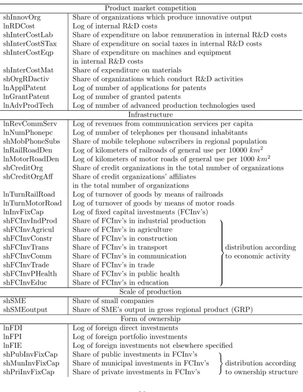
8. Control variables. We also aim to test some general hypothesis on regional socio-economic characteristics stimulating innovations. It is of par-ticular interest to investigate whether innovations are rather attributed to economically strong regions with large GRPs and budget revenues. Among variables tested are long term assets value, shares of urban population, un-employment and criminal activity. The full list of variables can be found in Table 6 in Appendix 7.1.
Innovations can be explained by the economic performance of companies, investments in infrastructure, and product market competition. However, they also induce improvements in economic performance, further investments in infrastructure and increase market competition (Cainelli et al. 2006). Therefore, we face the problem of a potential simultaneity bias. In order to tackle this problem, we use the instrumental variable approach in the context of a dynamic model specification.
2.2
Model Specification
In spite of the huge number of models proposed to explain the innovation process, there is no generally accepted model available encompassing all the factors of interest. Reviewing a great diversity of models, Forrest (1991) suggested some essential characteristics for a comprehensive model. First of all, the model should be nonlinear capturing an interrelationship of various stages of innovative activity. Then, it should include “identifiable” inputs and outputs. In addition, the generalized model must incorporate external effects, e.g., market competition and indicators of socio-economic environment. After all, the model should take into account the possible heterogeneity of regions. In order to set up such a generalized model, we consider the modified Cobb-Douglas Knowledge Production Function (KPF) (Crescenziet al.2007,
p. 170). Transforming it into a log-linear form approximating the initial model with arguments according to the hypotheses stated above we obtain:
𝑙𝑛𝑌𝑖 =𝛼+𝛽1𝑙𝑛𝑃 𝑀 𝐶𝑖+𝛽2𝑙𝑛𝑆𝑀 𝐸𝑖+𝛽3𝑙𝑛𝐹 𝑂𝑖+𝛽4𝑙𝑛𝐸𝑃𝑖
+𝛽5𝑙𝑛𝐼𝑛𝑓 𝑟𝑎𝑖+𝛽6𝑙𝑛𝑆𝑝𝑖𝑙𝑙𝐴𝑏𝑠𝑖+𝛽7𝑙𝑛𝑆𝑝𝑖𝑙𝑙𝑁𝑖 (1) +𝛽8𝑙𝑛𝑀 𝑎𝑐𝑟𝑜𝑖+𝑢𝑖,
where:
𝑌𝑖 innovative output of region 𝑖; 𝛼 a constant;
𝑃 𝑀 𝐶𝑖 indicators of market competition in region 𝑖; 𝑆𝑀 𝐸𝑖 indicators of SME’s activity in region 𝑖; 𝐹 𝑂𝑖 proxies for ownership structure of companies; 𝐸𝑃𝑖 proxies for companies’ economic performance; 𝐼𝑛𝑓 𝑟𝑎𝑖 proxies for regional infrastructure development;
𝑆𝑝𝑖𝑙𝑙𝐴𝑏𝑠𝑖 a vector of regional socio-economic characteristics, which may
improve ability to absorb new knowledge;
𝑆𝑝𝑖𝑙𝑙𝑁𝑖 socio-economic characteristics in neighboring regions; 𝑀 𝑎𝑐𝑟𝑜𝑖 further control variables, which address
relevant socio-economic characteristics of region 𝑖.
Moving from the KPF to (1), we approximate the stock of initial knowl-edge by several proxies of regional socio-economic characteristics (𝑆𝑝𝑖𝑙𝑙𝐴𝑏𝑠𝑖),
e.g., the number of doctoral students and employees in R&D departments. The number of patent applications (Crescenzi et al.2007) is used as a proxy for the stock of initial knowledge in parallel with the number of patents granted. Furthermore, in the dynamic specification of the model we include the regional innovative output in the previous period (𝑌𝑖,𝑡−1) as an additional
proxy for the stock of knowledge. Regional R&D activity is proxied by some market competition indicators (𝑃 𝑀 𝐶𝑖), e.g., the internal R&D costs.
Due to the logarithmic transformation in (1), 𝛽 is an elasticity: the per-cent change in𝑌 as a function of the percent change in the respective variable. As the transformation can be applied only to strictly positive data, some of the variables have to be expressed as percentage shares or average values. For these variables, 𝛽 is a rate of proportional change in 𝑌 per unit change in the respective regressor.
Gathering dependent and explanatory variables in vector 𝑦 and matrix
𝑦=𝛼𝜄𝑁 +𝑋𝛽+𝑢, (2)
where 𝛼 is a scalar, 𝜄𝑁 stands for a 𝑁 ×1 vector of ones, 𝑋 is a 𝑘×𝑁
matrix of 𝑘 regressors and their values for 𝑁 regions, 𝛽 is a 𝑘×1 vector of their coefficients and 𝑢is a 𝑁 ×1 vector of residuals. Here we use the panel data subscripts 𝑖for regions and 𝑡 for time.
2.2.1 Static Model Specification
Application of the Hausman test (Hausman and Taylor 1981) to preliminary estimates of (2) indicates that regional fixed effects (𝜇𝑖) should be taken into
account. To deal with these fixed effects we first specify a static model (3), where 𝑍𝜇 stands for the matrix of regional dummies:
𝑦=𝛼𝜄𝑁 +𝑋𝛽+𝑍𝜇𝜇+𝜈. (3)
Transforming the data into deviations from individual means we perform the LSDV (least squares dummy variables) estimation, which is also known as within estimation:
𝑦𝑖𝑡−𝑦𝑖 =𝛽(𝑥𝑖𝑡−𝑥𝑖) + (𝜈𝑖𝑡−𝜈𝑖). (4)
Assuming that𝜈∼𝑖𝑖𝑑(0, 𝜎2)and strict exogeneity of𝑋, the LSDV is the best linear unbiased estimator and consistent.
2.2.2 Dynamic Model Specification
As we are concerned about potential endogeneity of some of our explanatory variables, we consider a dynamic model suggested by Blundell and Bond (1998) with instruments in levels especially suitable for panel data with short time dimensions:
𝑦𝑖𝑡 =𝛿𝑦𝑖,𝑡−1+𝑋𝑖𝑡𝛽+𝑍𝜇𝜇+𝜈𝑖𝑡. (5)
The GMM method for dynamic panel data models with not strictly ex-ogenous variables was developed by Arellano and Bond (1991), introducing some basic restrictions on the model, e.g., no serial correlation, and using values of 𝑦𝑖𝑡 and 𝑋𝑖𝑡 lagged two periods or more as instrumental variables
in equations with first-differences. Later, it was shown that this estimator is weak and biased (Alonso-Borrego and Arellano 1999). The system GMM procedure introduced by Blundell and Bond (1998) appears superior, as it imposes additional restrictions on the initial condition process. It adds lagged
differences of 𝑦𝑖𝑡 and 𝑋𝑖𝑡 as additional instruments in order to improve the
efficiency for short time-series samples.
We consider two scenarios, where the explanatory variables 𝑋 are con-sidered either as endogenous or predetermined. Depending on which of these assumptions is maintained, different numbers of lags and lagged differences as instruments are used in the system GMM estimation. To test the validity of the instruments we apply the Sargan test (ST). The details of the system GMM estimation procedure are presented in Appendix 7.2.2
3
The Model Selection Procedure
3.1
The Optimization Problem
Let us first clarify the basic approach to the optimization problem. Consider the following regression function:
𝑦𝑡 =𝛼+𝛽𝑥𝑜𝑝𝑡𝑡 +𝑢, (6)
where 𝑥𝑡 = (𝑥1,𝑡, ..., 𝑥𝑘,𝑡) is a 𝑘-dimensional vector of variables with 𝑥𝑜𝑝𝑡𝑡
being the subset of all possible regressors we seek to identify. This might be the ‘true’ model in a Monte Carlo simulation setting or an optimal approx-imation to the unknown real data generating process. A vector 𝜔 specifies which variables are included in the model. It assigns the value of one or zero to indicate the selected or not selected variables. To select a model IC are implemented,which rank alternative models according to their fitness,while taking into account a penalty for model complexity.
Over the last years IC became a standard instrument in model selection problems ranging from lag order selection in multivariate linear (VAR and VEC) and nonlinear (MS-VAR) autoregression models to selection between rival nonnested models (Winker and Maringer 2004, Gatu et al. 2008).
In this study we implement Akaike’s IC (AIC), the Bayesian IC (BIC) and the Hannan-Quinn IC (HQIC). All these criteria have a similar structure:
IC=𝑙𝑛(𝜎2) +𝑓(𝑘, 𝑛), (7) where 𝜎2 is the maximum likelihood estimation of the residual sum of
squares. The second term is a penalty for the number of included parameters (𝑘). This term also depends on the sample size (𝑛). In particular, 2𝑘/𝑛,
𝑘𝑙𝑛(𝑛)/𝑛 and 2𝑘𝑙𝑛(𝑙𝑛(𝑛))/𝑛 are the AIC, BIC and HQIC penalties.
2We also apply the system GMM estimation procedure implemented in Stata 10 as a
Imposing some weak assumptions on the model space (𝑥𝑖,𝑡 and 𝜀𝑖,𝑡)
ac-cording to the results of Sin and White (1996) it can be shown that the vector 𝜔𝑖 that minimizes the 𝐼𝐶 converges to 𝜔𝑡𝑟𝑢𝑒 with probability close to
1 as 𝑛 → ∞. But for this to be true, it is essential that the penalty term
𝑓(𝑘, 𝑛) → ∞ and 𝑓(𝑘, 𝑛)/𝑛 → 0 as 𝑛 → ∞. In this sense, BIC and HQIC are consistent, while AIC is inconsistent.
In addition to the penalty for model complexity, we impose the constraint that at least one regressor from each group of variables specified in (1) is in-cluded. This constraint is enforced by imposing an additional multiplicative penalty (𝑝𝑗) to the objective function (7) in an optimization procedure. The
penalty increases over the iterations of the optimization algorithm to make sure that eventually the constraint is satisfied. This constraint is optional, as we might realize that no statistically significant variable is present for a par-ticular group. Furthermore, for the dynamic specification of the model the objective function is multiplicated by an additional penalty term (𝑝𝑒𝑛𝑆𝑇) de-rived from the results of the Sargan test to ensure that only valid instrument variables are considered:
IC= (𝑙𝑛(ˆ𝜈2) +𝑓(𝑘, 𝑛)) ( 1 + 8 ∑ 𝑗=1 𝑝𝑗 ) (1 +𝑝𝑒𝑛𝑆𝑇), (8)
where𝑗 stands for a group of variables and𝜈ˆdenotes residuals from the two-step estimator (see Appendix 7.2) and
𝑝𝑒𝑛𝑆𝑇 =
{
0 if 𝑆𝑇𝑝𝑟𝑜𝑏>0.1 1/𝑆𝑇𝑝𝑟𝑜𝑏 otherwise,
(9) where 𝑆𝑇𝑝𝑟𝑜𝑏 is the probability value of the Sargan test.
3.2
Heuristic Algorithms
Quality and precision of econometric estimation is crucially dependent on detecting the global optimum of any objective function. Breiman (2001) demonstrates the so called “Rashomon Effect”, where different model specifi-cations with very similar IC values provide different conclusions. Minimizing objective function (8) is not as simple as it might seem at first sight. In fact, the search space of candidate models is discrete (Winker (2001, p. 192)). The full enumeration of all possible solutions is only feasible for a small dimen-sional 𝑥𝑡. In our empirical problem the selection is made out of 80 variables
resulting in 280 potential sub-models. Therefore, the full enumeration is in-feasible even using efficient algorithms (Gatu et al. 2008).
In the last two decades, new nature-inspired optimization methods have become available. For an overview of these optimization techniques see Winker (2001) and Gilli and Winker (2004). In the following we describe the two heuristic methods implemented, the Threshold Accepting (TA) and the Genetic Algorithms (GA).
3.2.1 Threshold Accepting
The TA algorithm, suggested by Dueck and Scheurer (1990), is a refinement of classical local search procedures. In contrast to a local search, where a new solution is accepted only if an improvement is realized, TA also accepts uphill moves as long as they do not exceed a given threshold value 𝜏. A pseudocode of the TA implementation can be found in Algorithm 1.
Algorithm 1 Pseudocode for Threshold Accepting.
1: Generate at random a solution𝜔0, initialize𝐼
𝑚𝑎𝑥 and𝜏
2: for𝐼= 1to𝐼𝑚𝑎𝑥 do
3: Generate at random neighbor𝜔1∈ 𝒩(𝜔0)
4: if 𝑓(𝜔0)−𝑓(𝜔1)< 𝜏 then
5: 𝜔0=𝜔1
6: end if
7: Reduce𝜏
8: end for
In TA we generate an initial solution 𝜔0 as a vector of 𝑘 binary
compo-nents corresponding to our 𝑋 variables. A fixed number of variables (here it is 2) is included in each group and they are randomly distributed across the vector. Generating an initial solution at random instead of constructing it based on, e.g., empirical evidence or expectations, has the advantage that the algorithm will not start with a possible local optimum.
We generate a new solution𝜔1 by exchanging two randomly chosen
com-ponents with comcom-ponents located in a close neighborhood,3 in particular in the radius of three vector components. We choose the ’neighbor’ by means of the uniform random distribution and if it has the same value as the first component, than its value is changed to an opposite binary value: from 0 to 1 and vice versa. The same is true if the ’neighbor’ turns out to be the initially chosen component.
To generate an effective threshold sequence for all three IC, we obtain threshold values by a data driven method (Winker 2001, p. 170). To this end, we calculate absolute differences between the initial and new objective
3Changing the value of one element makes the algorithm slower and, e.g., of four
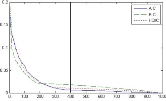
Figure 1: Threshold sequences from local deviation simulations.
function values with no penalty term for the number of groups included, and arrange them in decreasing order (Figure 1).
We use only a lower fraction𝜚of these sequences. This is made to improve the performance of the algorithm and not to accept solutions almost arbi-trarily during the early iterations. The vertical line in Figure 1 corresponds to 𝜚= 0.6 selected based on tuning experiments.
As TA is a stochastic process it may find the best possible solution in the search space and then loose it during the searching procedure. To avoid this, the best found solution is saved.
3.2.2 Genetic Algorithms
Unlike TA, GA, proposed by Holland (1975), are population based heuris-tic methods that operate on a set of solutions (population). Thus, a GA investigates the search space in many directions simultaneously so that the probability of getting stuck into a local optimum is reduced.
The members in the GA population (chromosomes) are represented as bit strings, in which each position (gene) has two possible values: 1 and 0. In each generation GA replaces parts of a population with new chromo-somes (children) aimed to represent better solutions for a particular problem. Children are generated using a crossover mechanism, that combines parts of chromosomes (parents), and mutation, that randomly changes genes in
chro-mosomes. For optimal model selection we implement the GA pseudocode described in Algorithm 2.
Algorithm 2 Pseudocode for Genetic Algorithms.
1: Generate initial population𝐾of solutions, initialize𝐺𝑚𝑎𝑥 and𝐶
2: for𝑔= 1to𝐺𝑚𝑎𝑥 do
3: Sort chromosomes in K
4: Select𝐾′ ⊂𝐾 (parents), select𝐾∗⊂𝐾 (elitist) 5: initialize𝐾′′=∅ (set of children)
6: for𝑐= 1to 𝐶do
7: Select individuals𝑥𝑝𝑎𝑟𝑒𝑛𝑡1 and𝑥𝑝𝑎𝑟𝑒𝑛𝑡2 at random from 𝐾′
8: Apply cross-over to𝑥𝑝𝑎𝑟𝑒𝑛𝑡1and𝑥𝑝𝑎𝑟𝑒𝑛𝑡2 to produce𝑥𝑐ℎ𝑖𝑙𝑑
9: 𝐾′′=𝐾′′∪𝑥𝑐ℎ𝑖𝑙𝑑
10: end for
11: 𝐾= (𝐾′, 𝐾′′)
12: Mutate𝐾 ∖ 𝐾∗ at 8 random points
13: end for
𝐾 is a matrix of 𝑝 initial solutions. We use 𝑝 = 500 considering this number to be large enough to screen the search space in different directions and at the same time small enough to allow for effective sorting and selection of the best solutions.4 As in TA, chromosomes in the initial population are generated with a fixed number of included variables, randomly distributed over the vectors. Thereafter, the population is sorted in an ascending order according to the objective function value. Then, the 50% of the chromosomes with the best target values (parents, 𝐾′) are transferred to the new popula-tion. We also select the ten best (elitist) chromosomes (𝐾∗). Based on 𝐾′
we construct new chromosomes (children) by crossing them over. Generating children we allow parents with superior objective values to be selected more often. First, we select 200 parents at random with an equal probability for the parents to be selected and generate 200 children. Then, the 40 parents with the best objective values generate 40 more children. The 10 last children are generated from the elitist solutions by changing at random one gene.
In the implementation we compare two crossover mechanisms: single-point crossover and uniform crossover. In the single-point crossover two parents are split at a random gene (crossover-point). From the split parts two new children are generated by combining the first part of one parent with the second part of the other parent. The crossover-point is placed between the second and the next to last genes (Kapetanios 2007).
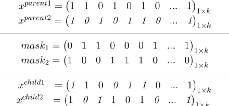
In contrast, in the uniform crossover parents may be split not only at one particular gene, but at each gene. With probability 𝑃0 we swap genes from
4We also tested populations of 100, 300 and 1000 solutions and found that the
𝑥𝑝𝑎𝑟𝑒𝑛𝑡1 =( 1 1 0 1 0 1 0 ... 1) 1×𝑘 𝑥𝑝𝑎𝑟𝑒𝑛𝑡2 =(1 0 1 0 1 1 0 ... 1) 1×𝑘 ——————————————————————— 𝑚𝑎𝑠𝑘1 = ( 0 1 1 0 0 0 1 ... 1)1×𝑘 𝑚𝑎𝑠𝑘2 = ( 1 0 0 1 1 1 0 ... 0) 1×𝑘 ——————————————————————— 𝑥𝑐ℎ𝑖𝑙𝑑1 =(1 1 0 0 1 1 0 ... 1)1×𝑘 𝑥𝑐ℎ𝑖𝑙𝑑2 =(1 0 1 1 0 1 0 ... 1) 1×𝑘
Figure 2: The uniform crossover mechanism.
two parents in a child. The uniform crossover can be presented as generating a mask of zeros and ones (see Figure 2), indicating for each gene from which parent it has to be taken. We set 𝑃0 = 0.5 resulting in equal probability for
each entry in the masks.
Performance analysis of the uniform crossover based on several binary function optimization problems can be found in Fogel (2006). It was shown that the uniform crossover outperforms both one- and two-point crossover mechanisms on average.
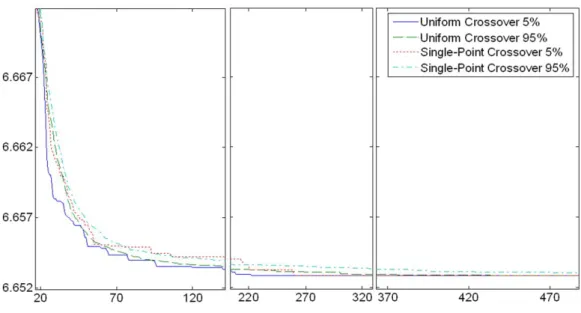
Testing both the single-point and uniform crossover for this particular problem based on repeated and independent Monte-Carlo simulations with 500 restarts we see that the uniform mechanism provides high quality so-lutions more reliably. The 95th percentiles of the results for the uniform crossover converge to the minimum value found in all replications (see Fig-ure 3), whereas for the single-point crossover a difference between the 5th and the rest 95th percentiles persists.5
The uniform crossover might be criticized for destroying superior chromo-some structures. We avoid this problem by preserving elitist solutions and, thus, screening the search space in a more efficient way.
After a new population is formed, mutation is applied at eight random genes with a probability of 50%.6 Mutation is applied to the whole new
population𝐾 except for the 10 elitist solutions and the 10 children generated from the elitist solutions by mutation. This procedure is repeated for a given number of generations 𝐺𝑚𝑎𝑥.
5In Figure 3, all objective function values accepted by the GA lie within the interval
between 6.65 and 6.72.
6We examined different number of genes and rates of mutation as well. By reducing the
number of genes or the probability of mutation, the computational time increases, while increasing both values increases the risk to miss high quality solutions.
Figure 3: Results of the single-point and uniform crossover.
4
Monte-Carlo Study
4.1
The Data Generating Process
In order to assess the performance of the implemented heuristic methods with an objective function as described in equations (7) and (8) we generate artificial data based on the panel dataset of Rosstat. First, a set of regressors (𝑋𝑀 𝐶) is randomly drawn from the database. Then, regression coefficients
(𝛽𝑀 𝐶) are estimated based on the dependent variable (𝑦). Finally, a new
dependent variable (𝑦𝑀 𝐶) is generated using the estimated coefficients adding
an identically and independently distributed error term:
𝑦𝑀 𝐶 =𝑋𝑀 𝐶𝛽𝑀 𝐶+𝜀, 𝜀 ∼𝑁(0, 𝜎𝜀2), (10)
where 𝜎2
𝜀 is the variance of the residuals.
Using a Data Generating Process (DGP) mimicking the empirical data, i.e., also with a cross-section dimension of 75 and eight time periods, we expect that the performance of the heuristics and the IC estimated based on this Monte-Carlo study is a good approximation for our real data problem.
4.2
Simulation Results
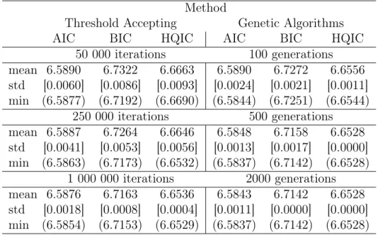
Table 1 presents results of TA and GA computational performance. The two algorithms are compared in terms of mean and minimum objective function
values and standard deviations. The descriptive results are obtained based on 10 restarts for each algorithm. The number of iterations for TA is taken equal to the number of chromosomes times the number of generations for GA resulting in the same number of function evaluations for both algorithms.
Table 1: Performance of the algorithms for different computing times. Method
Threshold Accepting Genetic Algorithms AIC BIC HQIC AIC BIC HQIC
50 000 iterations 100 generations mean 6.5890 6.7322 6.6663 6.5890 6.7272 6.6556 std [0.0060] [0.0086] [0.0093] [0.0024] [0.0021] [0.0011] min (6.5877) (6.7192) (6.6690) (6.5844) (6.7251) (6.6544) 250 000 iterations 500 generations mean 6.5887 6.7264 6.6646 6.5848 6.7158 6.6528 std [0.0041] [0.0053] [0.0056] [0.0013] [0.0017] [0.0000] min (6.5863) (6.7173) (6.6532) (6.5837) (6.7142) (6.6528) 1 000 000 iterations 2000 generations mean 6.5876 6.7163 6.6536 6.5843 6.7142 6.6528 std [0.0018] [0.0008] [0.0004] [0.0011] [0.0000] [0.0000] min (6.5854) (6.7153) (6.6529) (6.5837) (6.7142) (6.6528)
For TA with an increasing number of iterations we observe that mean, minimum objective function values and standard deviations decrease for all three information criteria (see Table 1).
For GA we obtain similar results, though the improvement is moderate. Comparing the results for the two heuristics we see that GA is able to find a good solution already with a relatively small number of generations (in particular, with 500 generations as it is seen from Table 1). Increasing the computational time up to 2 000 generations mainly reduces the variance of the results. Further increases of computational time (e.g., up to 5 000 000 iterations for TA and 10 000 generations for GA) do not improve the results significantly. As a result we conclude that GA appears superior to TA for this particular problem. First, the GA is about 20 percent faster than the TA for a comparable number of iterations.7 Second, GA provides us with
7Both algorithms are implemented using Matlab 7.7 on a Pentium IV 2.67 GHz. The
CPU time needed for 2 000 generations of the GA is about 700 s, while the TA implemen-tation with 1 000 000 requires 850 s. The small difference in CPU time is due to the more complex generation of neighbors for the TA as described above.
smaller standard deviations and slightly better objective function values (in terms of both mean and minimum values).
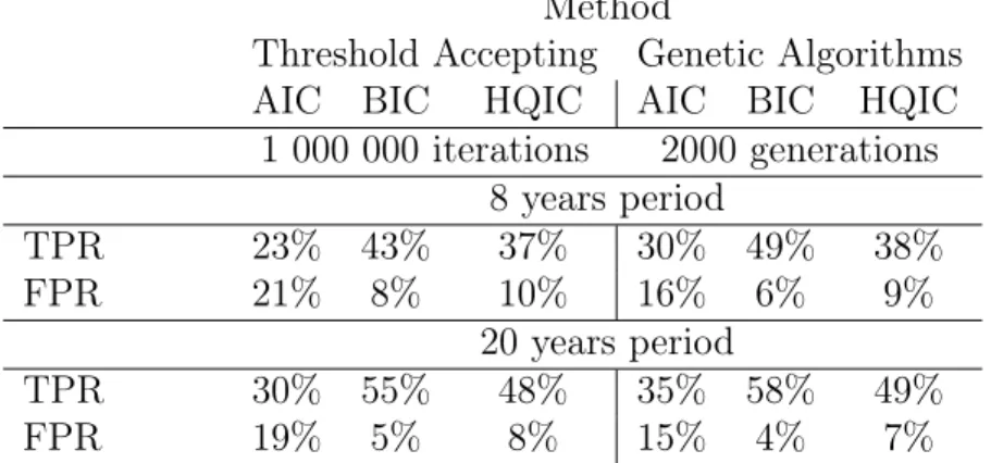
Now, to test the performance of our algorithms with an objective func-tion of type (8) in detecting ’true’ variables we run the algorithms for ten different artificial sets of data with eight ’true’ variables in each dataset. The simulation results are compared using the True Positive Rate (TPR) and the False Positive Rate (FPR)8 in the upper panel of Table 2.
Table 2: Performance of the algorithms. Method
Threshold Accepting Genetic Algorithms AIC BIC HQIC AIC BIC HQIC 1 000 000 iterations 2000 generations 8 years period TPR 23% 43% 37% 30% 49% 38% FPR 21% 8% 10% 16% 6% 9% 20 years period TPR 30% 55% 48% 35% 58% 49% FPR 19% 5% 8% 15% 4% 7%
As expected the objective function based on the Akaike criterion accepts too many ’false’ variables. Accepting on average 19-20 variables, AIC cor-rectly defines approximately 4 variables. BIC and HQIC significantly out-perform AIC, accepting less false variables (on average 8 and 11 regressors in total, respectively). As it is clear from Table 2 BIC is the most efficient IC in declining ’false’ variables, while HQIC regularly allows for more ’incorrect’ variables in the final solution. It is also evident that similarly to objective values, GA provides us with slightly better results than TA.
We believe that the main reason for the limited efficiency of all IC in Table 2 is the relatively small sample size: 75 regional observations for a period of eight years are not sufficient for the IC to identify the ’true’ model. Analyzing the data for eight years and using an optimization technique we find an IC-value smaller than the one corresponding to the ’true’ model.
In order to test the performance of the IC for a larger sample size, we artificially increase the time-series dimension: we select ’blocks’ from the dataset at random points (from 1 to 8) and add them to the current dataset.
8TPR is the percentage of ’true’ regressors from all regressors selected. FPR is the
Selecting the blocks at the same point for all variables, we produce a new dataset of 20 years. Although the dynamic structure of these artificial data differs from the one of the real data, we might still use them to test the performance of the selection criteria for larger sample sizes. Results of these experiments are presented in the lower panel of Table 2. It is obvious that the performance for all IC is significantly improved. Unfortunately, actual data for a longer period is not available for Russia.
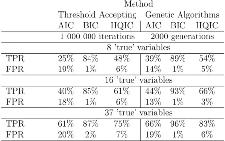
Table 3: Performance of the algorithms with no group penalty. Method
Threshold Accepting Genetic Algorithms AIC BIC HQIC AIC BIC HQIC 1 000 000 iterations 2000 generations 8 ’true’ variables TPR 25% 84% 48% 39% 89% 54% FPR 19% 1% 6% 14% 1% 5% 16 ’true’ variables TPR 40% 85% 61% 44% 93% 66% FPR 18% 1% 6% 13% 1% 3% 37 ’true’ variables TPR 61% 87% 75% 66% 96% 83% FPR 20% 2% 7% 19% 1% 6%
Considering again the original structure with eight periods, we also ana-lyze the performance of the IC when no penalties on the number of groups included are introduced (see Table 3). Thus, in the Monte-Carlo experiment with eight ’true’ variables, one from each group, BIC selects four variables on average with three to four of them correct and HQIC selects eight variables on average with four to five correct, accepting more false regressors. Increas-ing the number of a priori ’true’ variables the algorithms marginally increase the number of selected variables, improving their performance in terms of both: the TPR and FPR. For example, for 37 ’true’ variables (five variables in each group except of scale of production) HQIC selects 14 variables with 12 correct. However, it is obvious that for all IC this effect is accompanied with an increase of the number of true variables not included in the final model. This is also due to the finite sample size, where the asymptotic properties of the IC can be observed to a limited extent. In Table 3 it is also clear that GA have a tendency to select less variables for all the IC used, including less
true variables and rejecting more false variables. These facts should be taken into account when interpreting the results in Section 5.
5
Empirical Results on the Example of Russia
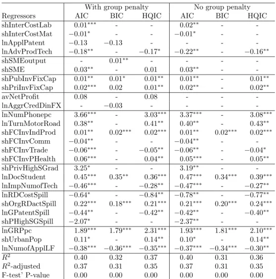
Based on the Monte-Carlo simulation results, we apply the superior GA algorithm on the database of Russian regions in order to specify the log-linear model of the form given in equation (1). We use the objective function (7)-(8) with AIC, BIC and HQIC with and without the penalty term on groups of variables included. The empirical results are obtained by running the GA 10 times with 2 000 generations for each IC. We only present the model specifications related to the smallest objective function values. Results for the static model are provided in Table 4 and for the dynamic model in Table 5.
The models obtained are similar in terms of variables included for all running sessions, but differ significantly between static and dynamic model specifications. Comparing the results in Tables 4 and 5 it is clear that the regression coefficients are different for most variables included in both spec-ifications. A good example to consider here is the GRP per capita. In the static model this variable has a strongly significant coefficient: 1% increase in the regressor is associated, ceteris paribus, with approximately 2% increase in the innovative output. But GRP can hardly be considered as exogenous with respect to the regional innovative performance. Considering this indica-tor as endogenous changes the result: in the GMM estimation the variable is estimated with an inverted sign and there is less evidence that it has a signif-icant effect on the dependent variable. In fact, in regions with ex ante high GRP per capita, e.g., regions in the North of Ural extracting oil, companies may have less incentives to innovate due to a different regional specialization. Therefore, in the following we concentrate on the system GMM estimation results, keeping the within estimation for a comparison.
An argument supporting the relevance of the obtained results is the fact that the set of regressors included is relatively stable for both assumptions on predetermined and endogenous variables. Another evidence for this is the fact that statistically significant9 variables are included with and without the
penalty on the number of groups included, while insignificant variables are dropped in specifications without this penalty.
According to the results in Table 5 the number of granted patents and
9The significance test is based on asymptotic standard errors for the one-step
estima-tor, which are seen to be more reliable if the residuals obtained from the estimator are heteroscedastic (see Arellano and Bond (1991) and Blundell and Bond (1998)).
Table 4: Within estimation results.
With group penalty No group penalty Regressors AIC BIC HQIC AIC BIC HQIC shInterCostLab 0.01∗∗∗ - - 0.02∗∗ - -shInterCostMat −0.01∗ - - −0.01∗ - -lnApplPatent −0.13 −0.13 - - - -lnAdvProdTech −0.18∗∗ - −0.17∗ −0.22∗∗ - −0.16∗∗ shSMEoutput - 0.01∗∗ - - - -shSME 0.03∗∗ - 0.01 0.03∗∗ - -shPubInvFixCap 0.01∗∗ 0.01∗ 0.01∗∗ 0.01∗∗ - 0.01∗∗ shPriInvFixCap 0.02∗∗∗ 0.02 0.01∗∗ 0.02∗∗ - 0.02∗∗ avNetProfit 0.08 - 0.08 - - -lnAggrCredDinFX - −0.03 - - - -lnNumPhonepc 3.66∗∗∗ - 3.03∗∗∗ 3.37∗∗∗ - 3.08∗∗∗ lnTurnMotorRoad 0.38∗∗ - 0.41∗∗ 0.40∗∗ - 0.43∗∗ shFCInvIndProd 0.01∗∗ 0.02∗∗∗ 0.02∗∗∗ 0.01∗∗ 0.02∗∗∗ 0.02∗∗∗ shFCInvComm −0.04∗∗ - - −0.04∗∗ - -shFCInvTrade −0.06∗∗∗ - −0.05∗∗ −0.06∗∗ - −0.04∗ shFCInvPHealth 0.06∗∗∗ - 0.04∗∗ 0.05∗∗∗ - 0.05∗∗ shPrivHighSGrad 3.25∗ - - 3.19∗∗ - -lnDocStudent 0.45∗∗∗ 0.35∗∗ 0.36∗∗∗ 0.47∗∗∗ 0.34∗∗∗ 0.39∗∗∗ lnImpNumofTech −0.46∗∗∗ - −0.28∗∗ −0.47∗∗∗ - −0.27∗∗ lnRDCostSpill −0.64∗ - −0.84∗∗ −0.78∗∗ - −0.77∗∗ shOrgRDactSpill 0.22∗∗∗ 0.18∗∗∗ 0.21∗∗∗ 0.21∗∗∗ 0.20∗∗∗ 0.24∗∗∗ lnGPatentSpill −0.44∗∗ - −0.42∗∗ −0.42∗∗ - −0.40∗∗ shPHighSGSpill −2.07∗ - - −2.37∗∗ - -lnGRPpc 1.89∗∗∗ 1.79∗∗∗ 2.31∗∗∗ 1.93∗∗∗ 1.81∗∗∗ 2.10∗∗∗ shUrbanPop 0.11∗ - 0.14∗∗ 0.10∗ - 0.14∗∗ lnNumofApplLF −0.38∗∗∗ −0.36∗∗∗ −0.35∗∗∗ −0.37∗∗∗ −0.34∗∗∗ −0.30∗∗ 𝑅2 0.40 0.32 0.37 0.40 0.31 0.36 𝑅2-adjusted 0.37 0.31 0.35 0.37 0.31 0.35 F-test’ P-value 0.00 0.00 0.00 0.00 0.00 0.00
the number of advanced production technologies used have, ceteris paribus, a positive effect on the regional innovative output. This result does not allow us to make any statement about the state of competition and its impact on the innovative activity. This finding rather provides us with an indirect estimate of knowledge spillovers within the limits of one region: new patents and technologies are widely seen as an instrument of knowledge transfer.
In conjunction to this result it is useful to consider the results on the hy-pothesis of knowledge spillovers from neighbor regions. The positive spillover effect of the innovative output in neighboring regions is contrasted with the negative effect of the number of granted patents. The positive influence of the value of innovative products in neighboring regions can be considered as plausible: a good or a service is a data carrier itself, and being exported can transfer knowledge to companies in neighboring regions.
On the contrary, the negative regression coefficient of the granted patents is a surprising result, as empirical evidence from the US and Western Eu-rope confirms patents as an instrument of knowledge diffusion (Bacchiocchi and Montobbio 2009). One might interpret this as a result of the property rights policy: technologies or goods patented in one region are protected from copying in neighbor regions. In this case, technologies implemented to produce innovative products in neighbor regions need to be either very close or even the same, which is a very strong assumption. Another explanation for this may be a concentration of Russian innovative companies in a few ’special economic zones’ (RusSEZ) with certain tax reliefs and further bene-fits for innovative companies. By this, these regions absorb production from neighbor regions instead of transferring knowledge.
Based on this result one might conclude that knowledge is regionally bound in Russia and particular measures to develop inter-regional knowl-edge diffusion are worth to undertake. These two effects are found to be strongly significant and are included with all IC in the final model speci-fication. Remember that these results are obtained with the neighborhood concept we have chosen. It is also relevant for further examination to test this hypothesis with a different concept, allowing, e.g., for knowledge spillovers between Moscow and St. Petersburg. These two most innovative regions in Russia are also expected to exhibit spillover effects with each other.
For the ownership hypothesis a positive partial effect of foreign direct investment (FDI) is identified. This is one of the few robust findings of this effect for the Russian economy (Tytell and Yudaeva 2006). Notice that for the static model specification FDI was not selected, and in the dynamic model it is included by all IC with the exception of BIC. According to the Monte-Carlo simulations BIC rejects more true variables than the other IC. However, the effect of FDI is fairly low. This may be due to a broader definition
T able 5: System GMM estimation results. Endogenous regressors Predetermined regress o rs With group p enalt y No group p enalt y With group p enalt y No group p enalt y Regressors AIC BIC HQIC AIC BIC HQIC AIC BIC HQIC AIC BIC HQIC Lagged dep enden t v ariable 0 . 18 ∗∗∗ 0 . 19 ∗∗∗ 0 . 15 ∗∗∗ 0 . 19 ∗∗∗ 0 . 29 ∗∗∗ 0 . 24 ∗∗∗ 0 . 20 ∗∗∗ 0 . 24 ∗∗∗ 0 . 17 ∗∗∗ 0 . 19 ∗∗∗ 0 . 25 ∗∗∗ 0 . 17 ∗∗∗ shInno vOrg 0 . 04 ∗ -0 . 03 ∗ -0 . 02 -lnGran tP aten t 0 . 24 ∗∗∗ -0 . 21 ∗∗∗ 0 . 26 ∗ 0 . 26 ∗∗ 0 . 24 ∗∗ 0 . 22 ∗∗ 0 . 22 ∗ 0 . 17 ∗ 0 . 23 ∗ 0 . 22 ∗ 0 . 18 ∗ lnA dvPro dT ec h 0 . 21 ∗∗∗ 0 . 43 ∗∗∗ 0 . 30 ∗∗∗ 0 . 21 ∗∗ 0 . 29 ∗∗ 0 . 23 ∗∗ 0 . 29 ∗∗∗ 0 . 34 ∗∗∗ 0 . 29 ∗∗∗ 0 . 32 ∗∗∗ 0 . 25 ∗∗∗ 0 . 33 ∗∗ shSMEoutput 0 . 004 0 . 004 0 . 001 -0 . 002 0 . 004 0 . 004 -lnFDI 0 . 05 ∗∗ 0 . 05 ∗ 0 . 05 ∗ 0 . 04 ∗∗ -0 . 05 ∗∗ 0 . 03 ∗ -0 . 03 ∗ 0 . 04 ∗∗ -0 . 05 ∗∗ shPriIn vFixCap 0 . 01 -0 . 01 -0 . 01 ∗ 0 . 01 0 . 01 0 . 01 0 . 01 -0 . 01 ∗∗ shAggrNetPinGRP 0 . 02 ∗∗∗ 0 . 02 ∗∗∗ 0 . 02 ∗∗∗ 0 . 02 ∗∗∗ 0 . 03 ∗∗∗ 0 . 03 ∗∗∗ 0 . 02 ∗∗∗ 0 . 01 ∗ 0 . 02 ∗∗ 0 . 02 ∗∗∗ 0 . 02 ∗∗∗ 0 . 01 ∗ a vNetProfit 0 . 06 -0 . 09 -0 . 04 -lnAggrCredDinRu 0 . 08 0 . 09 0 . 08 0 . 02 -0 . 01 0 . 04 -0 . 05 -lnRailRoadDen 0 . 14 ∗∗ 0 . 15 ∗∗∗ 0 . 13 ∗∗∗ 0 . 11 ∗ 0 . 17 ∗∗ 0 . 15 ∗∗∗ 0 . 02 -lnT urnRailRoad 0 . 01 -lnT urnMotorRoad -0 . 21 0 . 24 0 . 34 ∗∗∗ 0 . 19 ∗∗∗ -0 . 15 ∗∗∗ lnIn vFixCap 0 . 26 0 . 51 0 . 22 0 . 34 -0 . 47 ∗ 0 . 49 ∗ 0 . 52 ∗ 0 . 49 ∗ 0 . 49 ∗∗∗ 0 . 50 ∗ shF CIn vPHealth 0 . 03 ∗∗ -0 . 05 ∗∗ 0 . 04 ∗∗ -0 . 02 ∗∗ -0 . 04 ∗∗∗ 0 . 04 ∗∗∗ -0 . 04 ∗∗∗ shPubGradOEI -− 0 . 04 ∗∗ − 0 . 04 ∗ − 0 . 06 ∗∗ − 0 . 07 ∗∗ − 0 . 05 ∗∗ − 0 . 05 ∗∗ − 0 . 05 ∗∗ − 0 . 05 ∗∗ − 0 . 04 ∗∗∗ − 0 . 05 ∗∗∗ − 0 . 04 ∗ lnP ostdo cStud − 0 . 23 -− 0 . 12 -− 0 . 10 -lnInnOutSpill 0 . 25 ∗∗∗ 0 . 26 ∗∗∗ 0 . 28 ∗∗∗ 0 . 24 ∗∗∗ 0 . 31 ∗∗∗ 0 . 29 ∗∗∗ 0 . 30 ∗ 0 . 19 ∗∗∗ 0 . 28 ∗∗∗ 0 . 25 ∗∗∗ 0 . 25 ∗∗∗ 0 . 24 ∗∗∗ lnGP aten tSpill − 0 . 33 ∗∗∗ − 0 . 26 ∗∗∗ − 0 . 31 ∗∗∗ − 0 . 29 ∗∗∗ − 0 . 36 ∗∗∗ − 0 . 33 ∗∗∗ − 0 . 44 ∗ − 0 . 26 ∗ − 0 . 33 ∗∗∗ − 0 . 31 ∗∗∗ − 0 . 31 ∗ − 0 . 31 ∗ lnGRPp c − 0 . 14 − 0 . 32 ∗ − 0 . 17 -lnGRP -0 . 27 0 . 39 0 . 14 -𝑅 2 0 . 89 0 . 88 0 . 89 0 . 88 0 . 87 0 . 88 0 . 88 0 . 88 0 . 89 0 . 88 0 . 87 0 . 88 𝑅 2-adjusted 0 . 88 0 . 87 0 . 88 0 . 88 0 . 87 0 . 88 0 . 88 0 . 87 0 . 88 0 . 88 0 . 87 0 . 88 Sargan T est P-v alue 1 . 00 1 . 00 0 . 99 1 . 00 1 . 00 1 . 00 1 . 00 1 . 00 0 . 99 1 . 00 1 . 00 1 . 00 ∗∗∗ , ∗∗ , ∗ Statistically significan t, resp ectiv ely , at the 1, 5 and 10% lev el
of innovation used by Rosstat, including new products and services, which are not offered or produced in the country, and processes, which increase efficiency of the production. Another reason may be the low FDI inflow itself in relation to GDP in Russia (Tytell and Yudaeva 2006).
For the hypothesis on financial performance the only significant indicator selected with all criteria is the share of aggregated net profits in GRP. How-ever, its regression coefficient is of a fairly small value. To draw any concrete conclusions, the hypothesis must be tested on microdata.
Similarly, for the hypothesis on adoption of new knowledge, only the share of graduates from other public educational institutions (technical schools, colleges, academies) is selected and is found to be significant. In this case, the regression coefficient is negative, demonstrating that the share of graduates has, ceteris paribus, a negative impact on the innovative success. Taken in relation to the total regional population this indicator varies from its value around 1%, having a marginal impact on the innovative output. Nevertheless, the evidence is not obvious as the graduates of these schools are expected to enhance technical innovations. The negative impact might be explained by a selection bias: other public educational institutions being less attractive for potential students in comparison to universities are less efficient in preparing good specialists.
Among indicators on infrastructure the density of rail roads and the turnover of motor roads have partial negative effects on the dependent vari-able. Though, their inclusion in the final model is dependent on the assump-tion on the initial condiassump-tions process (endogenous or predetermined regres-sors). Similar evidence is found for the investments in fixed capital. The only exception for this are the investments in public health services. This re-gressor has a significant partial positive impact for both assumptions on the initial condition process. So far, we do not have an exhaustive explanation for this. Thus, we find some evidence that different infrastructure indicators have a positive impact on the innovative performance of regions, but until now, it is impossible to draw more specific conclusions.
Finally, there is no significant indicator on scale of production. Besides, the hypotheses on impact of public, municipal and private forms of ownership are not confirmed (the latter is not significant). None of the control variables are found to be significant.
6
Conclusions and Outlook
In this paper the innovative performance of Russian regions is analyzed. The innovative process is described in numerous studies with sometimes contra-dictive results. As there is no generally accepted model available encompass-ing all the factors of interest, a generalized log-linear model based on the regional data of Rosstat is suggested.
We optimize the model structure by selecting only those variables, which are relevant according to the information criteria. It is demonstrated that the corresponding optimization problem is complex due to the large discrete search space. Therefore, no classical optimization methods can be applied.
To deal with this problem two heuristic optimization approaches are sug-gested: Threshold Accepting and Genetic Algorithms. They are shown to be able to find an optimum or at least a very good result in terms of the IC value with, respectively, 1 000 000 iterations and 2 000 generations on average.
Comparing the heuristics we argue that for this particular problem for a given CPU time, GA provides marginally better results than TA in terms of the mean, minimum values and variance.
One problem that becomes obvious for our application is the asymptotic behavior of the IC. A sample size of 600 observations is too small for the information criteria to identify the ’true’ model. Instead, only up to 50% of the true variables are detected in a MC simulation. Relaxing the constraint that at least one variable from each group of potential regressors has to be included reduces the number of false variables included in the final model substantially (especially for BIC). However, the problem of relevant variables possibly not selected by the IC remains open.
Taking the unobserved heterogeneity and possible endogeneity of regres-sors into account, we compare both static and dynamic model specifications using GA. In particular, for the dynamic model specification, the system GMM estimation is undertaken. Based on this comparison a series of hy-potheses on stimulating innovations is tested.
In conclusion, we argue that the heuristic methods based on the IC are effective methods of model selection. In the future we will enhance our model selection procedure enabling to distinguish between strict exogenous, predetermined and endogenous variables simultaneously. For further study remains also the incorporation of the optimal choice of moments that could efficiently explore linear GMM moment restrictions and reduce the variance of the estimator. Application of the algorithms on a different dataset, in particular with a larger number of cross and time-series observations and with more accurate proxies on the market competition, investment climate and other hypotheses, is also of interest.
References
Alonso-Borrego, C. and M. Arellano (1999). Symmetrically normalized instrumental-variable estimation using panel data. Journal of Business and Economic Statistics 17(1), 36–49.
Arellano, M. and S. Bond (1991). Some tests of specification for panel data: Monte Carlo evidence and an application to employment equations. Re-view of Economic Studies 58(2), 277–297.
Bacchiocchi, E. and F. Montobbio (2009). Knowledge diffusion from univer-sity and public research. a comparison between US, Japan and Europe using patent citations. Journal of Technology Transfer 34(2), 169–181. Bilbao-Osorio, B. and A. Rodriguez-Pose (2004). From 𝑅&𝐷 to innovation
and economic growth in the EU. Growth and Change 35(4), 434–455. Blundell, R. and S. Bond (1998). Initial conditions and moment restrictions
in dynamic panel data models.Journal of Econometrics87(1), 115–143. Blundell, R., R. Griffith and J. Van Reenen (1999). Market share, market value and innovation in a panel of British manufacturing firms. Review of Economic Studies 66, 529–554.
Breiman, L. (2001). Statistical modelling: the two cultures. Statistical Sci-ence 16(3), 199–231.
Bucci, A. and C. P. Parello (2009). Horizontal innovation-based growth and product market competition. Economic Modelling26(1-2), 213–221. Cainelli, G., R. Evangelista and M. Savona (2006). Innovation and economic
performance in services: a firm-level analysis. Cambridge Journal of Economics 30(3), 435–458.
Crescenzi, R., A. Rodriguez-Posa and M. Storper (2007). The territorial dy-namics of innovation: a Europe-United States comparative analysis.
Journal of Economic Geography 7(6), 673–709.
Dueck, D. and T. Scheurer (1990). Threshold accepting: a general purpose algorithm appearing superior to simulated annealing. Journal of Com-putational Physics 90, 161–175.
Fernandez, C., E. Ley and M. Steel (2001). Model uncertainty in cross-country growth regressions. Journal of Applied Econometrics 16, 563– 576.
Fogel, D. B. (2006). Evolutionary Computation: Toward a New Philosophy of Machine Intelligence. Wiley-IEEE Press. Hoboken, NJ.
Forrest, J. E. (1991). Models of the process of technological innovation. Tech-nology Analysis & Strategic Management 3(4), 439–453.
Funk, M. (2006). Business cycles and research investment.Applied Economics
38, 1775–1782.
Gatu, C., E. J. Kontoghiorghes, M. Gilli and P. Winker (2008). An efficient branch-and-bound strategy for subset vector autoregressive model se-lection. Journal of Economic Dynamics & Control32, 1949–1963. Gilli, M. and P. Winker (2004). Applications of optimization heuristics to
estimation and modelling problems. Computational Statistics & Data Analysis 47(2), 211–223.
Hausman, J. A. and W. E. Taylor (1981). Panel data and unobservable in-dividual effects. Econometrica 49(6), 1377–1398.
Hendry, D. F. and H. M. Krolzig (2005). The properties of automatic "GETS" modelling. The Economic Journal 115(502), C32–C61.
Holland, J.H. (1975). Adaptation in Natural and Artificial Systems. Univer-sity of Michigan Press. Cambridge, MA.
Hsu, N.-J., H.-L. Hung and Y.-M. Chang (2007). Subset selction for vector autoregressive processes using lasso. Computational Statistics & Data Analysis 52(7), 3645–3657.
Jefferson, G., A. G. Z. Hu, X. Guan and X. Yu (2003). Ownership, per-formance, and innovation in China’s large- and medium-size industrial enterprise sector. China Economic Review 14(1), 89–113.
Kapetanios, G. (2007). Variable selection in regression models using non-standard optimization of information criteria. Computational Statistics & Data Analysis 52(1), 4–15.
Klotz, S. (1997). Econometric models with spatial autocorrelation -an introductory survey. Jahrbücher f. Nationalökonomie u. Statistik
218(1+2), 168–196.
Kozlov, K. and K. Yudaeva (2004). Imitations and innova-tions in a transition economy. Technical report. BOFIT. www.bof.fi/bofit/seminar/bofcef05/innovations.pdf.
MacGarvie, M. (2001). The determinants of international knowledge diffusion as measured by patent citations. Economics Letters87, 121–126. Merivate, E. J. and J. C. Pernias (2006). Innovation complementarity and
scale of production. Journal of Industrial Economics 54(1), 1–29. Okui, R. (2009). The optimal choice of moments in dynamic panel data
models. Journal of Econometrics 151(1), 1–16.
Opitz, P. and T. Sauer (1999). Strategic technology alliances: a way to inno-vative enterprises in Russia?. Post-Communist Economies 11(4), 487– 501.
Penrose, R. (1956). On best approximate solutions of linear matrix equations.
Proceedings of the Cambridge Philosophical Society 52(1), 17–19. Perez-Amaral, T., G. M. Gallo and H. White (2003). A flexible tool for model
building: The relevant transformation of the inputs network approach (RETINA).Oxford Bulletin of Economics and Statistics65(1), 821–838. Porter, M. E. (2003). The economic performance of regions.Regional Studies
37(6-7), 549–578.
Rosenberg, N. R., R. Landau and D. C. Mowery (1992). Technology and the Wealth of Nations. Stanford University Press. Stanford, CA.
Savin, I. and P. Winker (2009). Forecasting Russian foreign trade compar-ative advantages in the context of a potential WTO accession. Central European Journal of Economic Modelling and Econometrics 1(2), 111– 138.
Schumpeter, J. A. (1943). Capitalism, Socialism and Democracy. Allen Un-win. London.
Sin, C.-Y. and H. White (1996). Information criteria for selecting possibly misspecified parametric models. Journal of Econometrics71(1-2), 207– 225.
Sölvell, Ö. (2008). Clusters - Balancing Evolutionary and Constructive Forces. Ivory Tower Publishers. Stockholm.
Tytell, I. and K. Yudaeva (2006). The role of FDI in Eastern Europe and New Independent States. Technical report. Centro Studi Luca d’Agliano Development Studies Working Paper No. 217. Milan.
Winker, P. (1999). Causes and effects of financing constraints at the firm level: Some microeconometric evidence. Small Business Economics
12, 169–181.
Winker, P. (2001).Optimization Heuristics in Econometrics: Applications of Threshold Accepting. Wiley. Chichester.
Winker, P. and D. Maringer (2004). Optimal lag structure selection in VAR and VEC models. In: New Directions in Macromodelling (A. Welfe, Ed.). pp. 213–234. Elsevier. Amsterdam.
7
Appendix
7.1
Variables Used in the Analysis
Table 6: List of tested explanatory variables. Product market competition
shInnovOrg Share of organizations which produce innovative output lnRDCost Log of internal R&D costs
shInterCostLab Share of expenditure on labor remuneration in internal R&D costs shInterCostSTax Share of expenditure on social taxes in internal R&D costs shInterCostEqp Share of expenditure on machines and equipment
in internal R&D costs
shInterCostMat Share of expenditure on materials
shOrgRDactiv Share of organizations which conduct R&D activities lnApplPatent Log of number of applications for patents
lnGrantPatent Log of number of granted patents
lnAdvProdTech Log of number of advanced production technologies used Infrastructure
lnRevCommServ Log of revenues from communication services per capita lnNumPhonepc Log of number of telephones per thousand inhabitants shMobPhoneSubs Share of mobile telephone subscribers in regional population lnRailRoadDen Log of kilometers of railroads of general use per 10000𝑘𝑚2
lnMotorRoadDen Log of kilometers of motor roads of general use per 1000𝑘𝑚2
shCreditOrg Share of credit organizations in the total number of organizations shCreditOrgAff Share of credit organizations’ affiliates
in the total number of organizations
lnTurnRailRoad Log of turnover of goods by means of railroads lnTurnMotorRoad Log of turnover of goods by means of motor roads lnInvFixCap Log of fixed capital investments (FCInv’s)
shFCInvIndProd Share of FCInv’s in industrial production ⎫ ⎬ ⎭
shFCInvAgricul Share of FCInv’s in agriculture shFCInvConstr Share of FCInv’s in construction
shFCInvTrans Share of FCInv’s in transport distribution according shFCInvComm Share of FCInv’s in communication to economic activity shFCInvTrade Share of FCInv’s in trade
shFCInvPHealth Share of FCInv’s in public health shFCInvEduc Share of FCInv’s in education
Scale of production shSME Share of small companies
shSMEoutput Share of SME’s output in gross regional product (GRP) Form of ownership
lnFDI Log of foreign direct investments lnFPI Log of foreign portfolio investments
lnFIE Log of foreign investments not elsewhere specified shPubInvFixCap Share of public investments in FCInv’s }
shMunInvFixCap Share of municipal investments in FCInv’s distribution according shPriInvFixCap Share of private investments in FCInv’s to ownership structure
shPrivPubMunOrg Share of privatized public and municipal organizations
shEqtInvFixCap Share of equity in FCInv’s } distribution according shBCrInvFixCap Share of bank credits in FCInv’s to source of finance
Economic performance
shAggrNetPinGRP Share of aggregated net profit of companies in GRP avNetProfit Average net profit of companies in roubles (m)
lnAggrCredDinRu Log of aggregated credit debts of companies in roubles
lnAggrCredDinFX Log of aggregated credit debts of companies in foreign currency avCredDinRu Average credit debts of companies in roubles (m)
avCredDinFX Average credit debts of companies in foreign currency (in roubles, m) Knowledge spillovers I
shPubHighSGrad Share of public high-school graduates in total population (TP) shPrivHighSGrad Share of private high-school graduates in TP
shPubGradOEI Share of graduates from other public educational institutions in TP shPrivGradOEI Share of graduates from other private educational institutions in TP shPubHStoAllHS Share of public graduates in all high-school graduates
shPubtoAllGrad Share of public graduates in all graduates from other educational institutions
lnRDstaff Log of the number of employees in R&D departments lnDocStudent Log of number of doctoral students
lnPostdocStud Log of number of postdoctoral students
shExpRWorld Share of export to the rest of the world relative to GRP shImpRWorld Share of import to the rest of the world relative to GRP shExpCIS Share of export to the CIS countries relative to GRP shImpCIS Share of import to the CIS countries relative to GRP lnExpNumofTech Log of number of contracts for export of technologies lnExpValofTech Log of value of contracts for export of technologies
lnExpEarnofTech Log of annual earnings of contracts for export of technologies lnImpNumofTech Log of number of contracts for import of technologies
lnImpValofTech Log of value of contracts for import of technologies
lnImpEarnofTech Log of annual earnings of contracts for import of technologies Knowledge spillovers II
lnInnOutSpill Log of value of innovative products in neighboring regions (NR) lnRDCostSpill Log of internal costs on R&D in neighboring regions in NR shOrgRDactSpill Share of organizations which conduct R&D activities in NR lnGPatentSpill Log of number of granted patents in NR
lnAdvPrTSpill Log of number of advanced production technologies used in NR shPHighSGSpill Share of public high-school graduates in the total population in NR lnRDstaffSpill Log of the number of employees in R&D departments in NR
Control variables lnGRP Log of GRP in current prices
lnGRPpc Log of gross regional product per capita in current prices lnRevConsBudg Log of revenues of regional consolidated budgets
lnValLTAssets Log of value of regional long term assets
shEmplPop Share of employable population in total population shUrbanPop Share of urban population in total population
shUnEmplPop Share of unemployed population (relative to employable population) lnNumofApplLF Log of number of applications for labor force
7.2
System GMM Estimation Technique
Here we will state the assumptions of the system GMM estimators applied. First, 𝜇𝑖 and 𝜈𝑖𝑡 are independently identically distributed so that
𝐸(𝜇𝑖) = 0; 𝐸(𝜈𝑖𝑡) = 0; 𝐸(𝜈𝑖𝑡𝜇𝑖) = 0; 𝑖= 1, ..., 𝑁; 𝑡 = 2, . . . , 𝑇 (11)
and there is lack of serial correlation, but not necessarily independence over time:
𝐸(𝜈𝑖𝑡𝜈𝑖𝑠) = 0; 𝑖= 1, ..., 𝑁; 𝑡= 2, . . . , 𝑇; ∀𝑡 ∕=𝑠. (12)
Following Blundell and Bond (1998) we also make the standard assump-tion concerning the initial condiassump-tions 𝑦𝑖1:
𝐸(𝑦𝑖1𝜈𝑖𝑡) = 0; 𝑖= 1, ..., 𝑁; 𝑡= 2, . . . , 𝑇. (13)
Conditions (11), (12), (13) are sufficient for the following(𝑇−1)(𝑇−2)/2
linear moment conditions to be valid:
𝐸[𝑦𝑖,𝑡−2Δ(𝜇𝑖 +𝜈𝑖𝑡)] = 0; 𝑡 = 3, . . . , 𝑇, (14)
whereΔ(𝜇𝑖+𝜈𝑖𝑡) = Δ𝑢𝑖𝑡 =𝑢𝑖𝑡−𝑢𝑖,𝑡−1 = Δ𝑦𝑖,𝑡−ˆ𝛿Δ𝑦𝑖,𝑡−1−Δ𝑋𝑖,𝑡𝛽ˆ.
Intro-ducing lagged values of 𝑦𝑖𝑡 as instruments, we estimate 𝛿 in first-differences
for datasets with a time-series dimension𝑇 ≥3. But as these estimations are biased (Alonso-Borrego and Arellano 1999), we need to make an additional mild stationarity assumption about the initial conditions 𝑦𝑖1 allowing the use
of an extended ’system GMM’ estimator that uses lagged differences of 𝑦𝑖𝑡
as instruments for equations in levels. This stationarity condition on 𝑦𝑖1
re-quires 𝐸[(𝑦𝑖1 − 1𝜇−𝛿𝑖 )𝜇𝑖] = 0 for 𝑖 = 1, . . . , 𝑁, so that 𝑦𝑖𝑡 converges towards
its mean 𝜇𝑖
1−𝛿 for each region from period 𝑡 = 2 onwards. This yields the
condition:
𝐸[Δ𝑦𝑖,𝑡−1𝜇𝑖] = 0; 𝑖= 1, . . . , 𝑁. (15)
If (11), (12), (13) and (15) hold, the additional(𝑇−1)(𝑇 −2)/2moment conditions are valid:
𝐸[Δ𝑦𝑖,𝑡−1(𝜇𝑖 +𝜈𝑖𝑡)] = 0; 𝑡 = 3, . . . , 𝑇. (16)
Together the moment conditions on equations in first-differences (14) and on equations in levels (16) yield the system GMM estimator (Blundell and Bond 1998).