Unsupervised Selection and Estimation of
Non-Gaussian Mixtures for High
Dimensional Data Analysis
Tarek Elguebaly
A Thesis in
The Department of
Electrical and Computer Engineering
Presented in Partial Fulf llment of the Requirements for the Degree of PhD (Electrical and Computer Engineering) at
Concordia University Montr´eal, Qu´ebec, Canada
June 2014
c
CONCORDIA UNIVERSITY SCHOOL OF GRADUATE STUDIES
This is to certify that the thesis prepared
By:
Entitled:
and submitted in partial fulfillment of the requirements for the degree of
complies with the regulations of the University and meets the accepted standards with respect to originality and quality.
Signed by the final examining committee:
Chair External Examiner External to Program Examiner Examiner Thesis Supervisor Approved by Chair of Department or Graduate Program Director
Tarek Elguebaly
Unsupervised Selection and Estimation of Non-Gaussian Mixtures for High Dimensional Data Analysis
PhD (Electrical and Computer Engineering)
Dr. Adel M. Hanna Dr. Fakhreddine Karray Dr. Hoi Dick Ng
Dr. Abdessamad Ben Hamza Dr. Walaa Hamouda
Abstract
Unsupervised Selection and Estimation of Non-Gaussian Mixtures for High
Dimensional Data Analysis
Tarek Elguebaly, Ph.D. Concordia University, 2014
Lately, the enormous generation of databases in almost every aspect of life has created a great demand for new, powerful tools for turning data into useful information. Therefore, researchers were encouraged to explore and develop new machine learning ideas and methods. Mixture models are one of the machine learning techniques receiving considerable attention due to their ability to handle eff ciently and effectively multidimensional data. Generally, four critical issues have to be addressed when adopting mixture models in high dimensional spaces: (1) choice of the probability density functions, (2) estimation of the mixture parameters, (3) automatic determination of the number of componentsM in the mixture, and (4) determination of what features best discriminate among the different components. The main goal of this thesis is to summarize all these challenging interrelated problems in one unif ed model.
In most of the applications, the Gaussian density is used in mixture modeling of data. Although a Gaussian mixture may provide a reasonable approximation to many real-world distributions, it is certainly not always the best approximation especially in computer vision and image process-ing applications where we often deal with non-Gaussian data. Therefore, we propose to use three highly f exible distributions: the generalized Gaussian distribution (GGD), the asymmetric Gaus-sian distribution (AGD), and the asymmetric generalized GausGaus-sian distribution (AGGD). We are motivated by the fact that these distributions are able to f t many distributional shapes and then can be considered as a useful class of f exible models to address several problems and applications in-volving measurements and features having well-known marked deviation from the Gaussian shape. Recently, researches have shown that model selection and parameter learning are highly de-pendent and should be performed simultaneously. For this purpose, many approaches have been suggested. The vast majority of these approaches can be classif ed, from a computational point of view, into two classes: deterministic and stochastic methods. Deterministic methods estimate the model parameters for a set of candidate models using the Expectation-Maximization (EM)
framework, then choose the model that maximizes a model selection criterion. Stochastic methods such as Markov chain Monte Carlo (MCMC) can be used in order to sample from the full a pos-teriori distribution withM considered unknown. Hence, in this thesis, we propose three learning techniques capable of automatically determining model complexity while learning its parameters. First, we incorporate a Minimum Message Length (MML) penalty in the model learning step per-formed using the EM algorithm. Our second approach employs the Rival Penalized EM (RPEM) algorithm which is able to select an appropriate number of densities by fading out the redundant densities from a density mixture. Last but not least, we incorporate the nonparametric aspect of mixture models by assuming a countably inf nite number of components and using Markov Chain Monte Carlo (MCMC) simulations for the estimation of the posterior distributions. Hence, the diff culty of choosing the appropriate number of clusters is sidestepped by assuming that there are an inf nite number of mixture components.
Another essential issue in the case of statistical modeling in general and f nite mixtures in particular is feature selection (i.e. identif cation of the relevant or discriminative features describ-ing the data) especially in the case of high-dimensional data. Indeed, feature selection has been shown to be a crucial step in several image processing, computer vision and pattern recognition applications not only because it speeds up learning but also because it improves model accuracy and generalization. Moreover, the learning of the mixture parameters ( i.e. both model selection and parameters estimation) is greatly affected by the quality of the features used. Hence, in this thesis, we are trying to solve the feature selection problem in unsupervised learning by casting it as an estimation problem, thus avoiding any combinatorial search. Finally, the effectiveness of our approaches is evaluated by applying them to different computer vision and image processing applications.
Acknowledgements
I owe my deepest gratitude to my supervisor, Dr. Nizar Bouguila, for his continuous support and encouragement throughout my graduate studies. It was an honor for me to work with such a wonderful advisor.
I would like to thank the members of my committee for their encouragement, insightful com-ments, and advices. Also I am thankful to my fellow lab-mates at Concordia University for their support, motivation and all the good time we had together. I am also grateful to Concordia Uni-versity and to the Natural Sciences and Engineering Research Council (NSERC) of Canada for supporting my research during my graduate studies.
Finally, I would like to thank my family for unconditional support throughout my studies, your endless love and care always encourage me.
Table of Contents
List of Tables ix
List of Figures xi
1 Introduction 1
1.1 Mixture Models . . . 3
1.1.1 Probability Density Function Selection . . . 3
1.1.2 Parameters Learning . . . 4
1.1.3 Selection of the number of components . . . 5
1.1.4 Feature Selection . . . 6
1.2 Contributions . . . 7
1.3 Thesis Overview . . . 8
2 Generalized Gaussian mixture models as a nonparametric Bayesian approach for clustering using class-specif c visual features 10 2.1 Introduction . . . 11
2.2 A Hierarchical Bayesian Model for Clustering and Feature Selection . . . 13
2.2.1 The Modeling Approach . . . 13
2.2.2 Bayesian Hierarchical Model . . . 15
2.3 Nonparametric Bayesian Learning . . . 17
2.3.1 Priors and Posteriors . . . 17
2.3.2 The Inf nite Model . . . 20
2.3.3 Complete Algorithm . . . 21
2.4 Experimental Results . . . 23
2.4.1 Distinguishing Paintings from Photographs . . . 23
2.4.2 Image and Video Segmentation . . . 25
2.5 Discussion . . . 34
3 Background subtraction using f nite mixtures of asymmetric Gaussian distributions and shadow detection 39 3.1 Introduction . . . 40
3.2 Finite AGM Model . . . 43
3.2.1 Maximum Likelihood Estimation of the Mixture Parameters . . . 44
3.2.2 Model Selection Using the Minimum Message Length Criterion . . . 46
3.2.3 The AGM Model Learning Algorithm . . . 49
3.3 Background Subtraction . . . 50
3.3.1 Adaptive AGM algorithm . . . 50
3.3.2 Shadow Detection Algorithm . . . 53
3.3.3 Results . . . 56
3.4 Discussion . . . 59
4 Finite asymmetric generalized Gaussian mixture models learning for infrared object detection 65 4.1 Introduction . . . 66
4.2 Finite Asymmetric Generalized Gaussian Mixture Model . . . 69
4.2.1 The Finite Mixture Model . . . 69
4.2.2 Maximum Likelihood Estimation of the Mixture Parameters . . . 70
4.2.3 Model Selection Using MML Criterion . . . 72
4.2.4 Complete AGGM Learning Algorithm . . . 76
4.3 Experimental Results . . . 76
4.3.1 Pedestrian detection . . . 77
4.3.2 Multiple-Target Tracking . . . 81
4.4 Discussion . . . 90
5 Simultaneous high-dimensional clustering and feature selection using Asymmetric mixture models 92 5.1 Introduction . . . 93
5.2 Feature Selection for Asymmetric Mixture Models . . . 94
5.3 Learning via EM and MML . . . 97
5.3.1 Parameter estimation using EM . . . 97
5.3.2 Model selection using MML . . . 99
5.3.3 The Complete learning algorithm . . . 100
5.4 Learning via RPEM . . . 101
5.5 Experimental Results . . . 105
5.5.1 Scene Categorization . . . 105
5.6 Discussion . . . 120 6 Conclusions 121 List of References 124 A 147 B 148 C 149 D 151 E 155
List of Tables
2.1 Average classif cation accuracies (%) (±standard deviation) obtained using differ-ent approaches for distinguishing paintings from photographs. IGM: inf nite Gaus-sian mixture, IGM + FS: inf nite GausGaus-sian mixture with feature selection, IGGM: inf nite generalized Gaussian mixture, IGGM + FS: inf nite generalized Gaussian
mixture with feature selection. . . 26
2.2 Errors (E1 andE2) calculation for the Berkeley dataset. . . 28
2.3 Errors (E1andE2) calculation for the 2 tested videos when using our inf nite model (IGGM+FS), f nite Gaussian mixture (GM), f nite Gaussian mixture with feature selection (GM+FS), f nite generalized Gaussian (GGM), f nite generalized Gaus-sian with feature selection (GGM+FS), inf nite GausGaus-sian mixture (IGM), inf nite Gaussian mixture with feature selection (IGM+FS) and inf nite generalized Gaus-sian (IGM). . . 33
2.4 Confusion matrices for the infrared facial expression recognition application using: (a) GM, (b) IGM, (c) GGM, (d) IGGM, (e) GM+FS, (f) IGM+FS, (g) GGM+FS, (h) IGGM+FS. . . 37
2.5 Accuracies and NMI when applying the 8 methods for the infrared facial expres-sion recognition. . . 38
3.1 Baseline Precision and Recall . . . 61
3.2 Dynamic Background Precision and Recall . . . 62
3.3 Camera Jitter Precision and Recall . . . 63
3.4 Intermittent Object Motion Precision and Recall . . . 63
3.5 Shadows Precision and Recall . . . 63
3.6 Thermal Precision and Recall . . . 64
3.7 Overall Precision and Recall . . . 64
4.1 Precision and Recall . . . 80
4.3 Multiple target tracking results. . . 90 5.1 The confusion matrix of the AGM-EM-MML for the UIUC sports event data set. . 109 5.2 The confusion matrix of the AGM-RPEM for the UIUC sports event data set. . . . 110 5.3 The confusion matrix of the AGGM-EM-MML for the UIUC sports event data set. 110 5.4 The confusion matrix of the AGGM-RPEM for the UIUC sports event data set. . . 110 5.5 The confusion matrix of the AGM-EM-MML for the 15 scenes categories data set. 111 5.6 The confusion matrix of the AGM-RPEM for the 15 scenes categories data set. . . 111 5.7 The confusion matrix of the AGGM-EM-MML for the 15 scenes categories data set.111 5.8 The confusion matrix of the AGGM-RPEM for the 15 scenes categories data set. . 112 5.9 The average accuracies (%) for the UIUC event data set. . . 113 5.10 The average accuracies (%) for the 15 categories data set. . . 113 5.11 Average precision and recall (%) of all the descriptor/Classif er combinations for
the JAFFE database. . . 119 5.12 Average precision and recall (%) of all the descriptor/Classif er combinations for
the Cohn- Kanade database. . . 119 5.13 Average precision and recall (%) of all the descriptor/Classif er combinations for
List of Figures
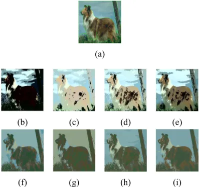
2.1 Sample images from each group. Row 1: Paintings, Row 2: Photographs. . . 25 2.2 Segmentation results for the f rst image from the Berkeley dataset. (a) GT, (b)
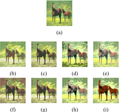
GM, (c) IGM, (d) GGM, (e) IGGM, (f) GM+FS, (g) IGM+FS, (h) GGM+FS, (i) IGGM+FS. . . 28 2.3 Segmentation results for the second image from the Berkeley dataset. (a) GT, (b)
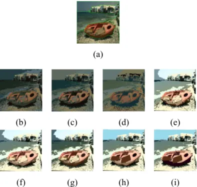
GM, (c) IGM, (d) GGM, (e) IGGM, (f) GM+FS, (g) IGM+FS, (h) GGM+FS, (i) IGGM+FS. . . 29 2.4 Segmentation results for the third image from the Berkeley dataset. (a) GT, (b)
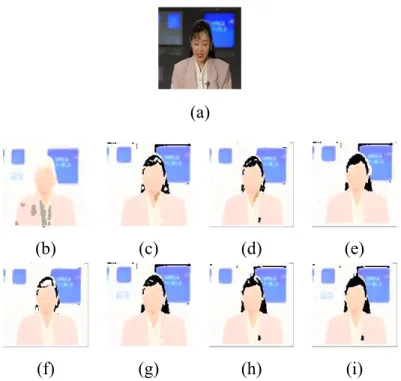
GM, (c) IGM, (d) GGM, (e) IGGM, (f) GM+FS, (g) IGM+FS, (h) GGM+FS, (i) IGGM+FS. . . 30 2.5 Sample image from Akiyo video. (a) Sample frame, (b) GM, (c) IGM, (d) GGM,
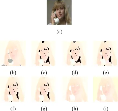
(e) IGGM, (f) GM+FS, (g) IGM+FS, (h) GGM+FS, (i) IGGM+FS. . . 31 2.6 Sample image from Suzie video. (a) Sample frame, (b) GM, (c) IGM, (d) GGM,
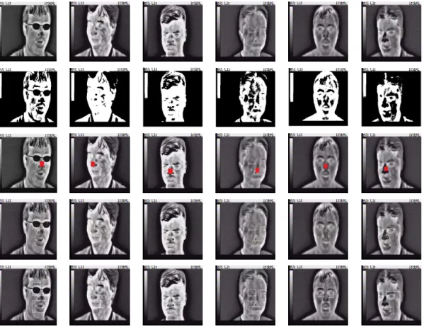
(e) IGGM, (f) GM+FS, (g) IGM+FS, (h) GGM+FS, (i) IGGM+FS. . . 32 2.7 Sample images from each group. Row 1: Surprise, Row 2: Happy, Row 3: Angry. . 35 2.8 Processing steps shown for sample images from each group. Row 1: sample
im-ages, Row 2: Thresholding, Row 3: Center location, Row 4: Interest points detec-tion, Row 5: Regions of interest extraction. . . 36 3.1 Probability density function of a pixel throughout a video sequence. . . 42 3.2 (a) Sample frame from Pets2006 video sequence in the baseline category, (b)
Stauf-fer et al. [2], (c) Zivkovic [3], (d) KaewTraKulPong et al. [4], (e) Evangelio et al. [5], (f) ELgammal et al. [6], (g) Nonaka et al. [7], (h) AGM, (i) AGM+SD. . . . 57 3.3 (a) Sample frame from Overpass video sequence in the dynamic background
cat-egory, (b) Stauffer et al. [2], (c) Zivkovic [3], (d) KaewTraKulPong et al. [4], (e) Evangelio et al. [5], (f) ELgammal et al. [6], (g) Nonaka et al. [7], (h) AGM, (i) AGM+SD. . . 58
3.4 (a) Sample frame from Badminton video sequence in the Camera Jitter category, (b) Stauffer et al. [2], (c) Zivkovic [3], (d) KaewTraKulPong et al. [4], (e) Evange-lio et al. [5], (f) ELgammal et al. [6], (g) Nonaka et al. [7], (h) AGM, (i) AGM+SD. 59 3.5 (a)Sample frame from Parking video sequence in the Intermittent Object Motion
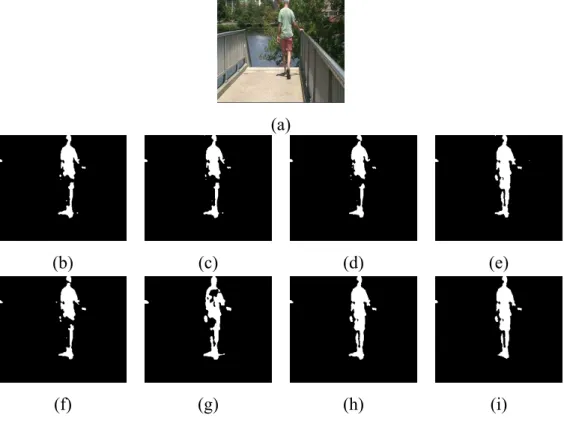
category, (b) Stauffer et al. [2], (c) Zivkovic [3], (d) KaewTraKulPong et al. [4], (e) Evangelio et al. [5], (f) ELgammal et al. [6], (g) Nonaka et al. [7], (h) AGM, (i) AGM+SD. . . 60 3.6 (a) Sample frame from PeopleInShade video sequence in the shadows category, (b)
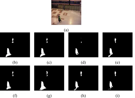
Stauffer et al. [2], (c) Zivkovic [3], (d) KaewTraKulPong et al. [4], (e) Evangelio et al. [5], (f) ELgammal et al. [6], (g) Nonaka et al. [7], (h) AGM, (i) AGM+SD. . . 61 3.7 (a) Sample frame from Corridor video sequence in the thermal category, (b)
Stauf-fer et al. [2], (c) Zivkovic [3], (d) KaewTraKulPong et al. [4], (e) Evangelio et al. [5], (f) ELgammal et al. [6], (g) Nonaka et al. [7], (h) AGM, (i) AGM+SD. . . . 62 3.8 Precision and Recall curves for : TheAGM and theAGM+SDwhen varyingT
andK. . . 64 4.1 (a) IR image, (b) Real and estimated (using GM, GGM and AGGM) histograms
for the IR image. . . 68 4.2 (a) IR image for f ve pedestrians in the presence of Haze, (b) GM, (c) IGM, (d)
GGM, (e) IGGM, and (f) AGGM. . . 78 4.3 (a) IR Image for six pedestrians on a very cloudy day, (b) GM, (c) IGM, (d) GGM,
(e) IGGM, and (f) AGGM. . . 79 4.4 (a) IR Image for six pedestrians on a rainy day, (b) MoG, (c) IMoG, (d) MoGG,
(e) IMoGG, and (f) MoAGG. . . 79 4.5 Some sample frames from the OSU Color-Thermal database. . . 82 4.6 (a) Color image, (b) IR image, (c) GM, (d) GGM, (e) IGGM, and (f) AGGM. . . . 85 4.7 (a) Color image, (b) IR image, (c) GM, (d) GGM, (e) IGGM, and (f) AGGM. . . . 85 4.8 (a) Color image, (b) IR image, (c) GM, (d) GGM, (e) IGGM, and (f) AGGM. . . . 86 4.9 Low level tracking example using the ellipse centroid metric. . . 87 4.10 System architecture. . . 89 4.11 Collision detection example. (a) Object before collision (b) Grouping and splitting
events identif ed. . . 89 5.1 Sample images from the UIUC sports event data set; (a) Snow-boarding, (b)
Sail-ing, (c) RowSail-ing, (d) Rock-climbSail-ing, (e) Polo, (f) Croquet, (g) Bocce, (h) Badminton.107 5.2 Sample images from the 15 categories data set; (a) Off ce, (b) Bedroom, (c) Open
country, (d) Highway, (e) Street, (f) inside-city, (g) Suburb-residence, (h) kitchen, (i) Coast, (j) Living-room, (k) Forest, (l) Mountain, (m) Tall-buildings, (n) Indus-trial, (o) Store. . . 108
5.3 Sample images for the seven emotions from the three datasets under consideration. First Row: JAFFE dataset, Second Row: Cohn-Kanade dataset, and Thrid Row: SFEW dataset. Facial expressions are: (a) Angry, (b) Disgust, (c) Fear, (d) Joy, (e) Neutral, (f) Sadness, and (g) Surprised. . . 115
Chapter
1
Introduction
Over the last decade, technological advances have brought an explosion of enormous data not only in size but also in dimension. These data pose a challenge to standard statistical methods and comparatively recently have received much attention. The importance of f nding a way to model and analyze multidimensional data lies in their usefulness in wide range of applications such as image processing and computer vision. Modeling and f nding valuable information in multidi-mensional data depend on recognizing complex patterns, regularities, and relationships in data. In recent years various algorithms were developed in the aim of automatically learning to rec-ognize complex patterns, and to produce intelligent decisions based on observed data. Machine learning is the branch of artif cial intelligence that offers a principled approach for developing and studying automatic techniques capable of learning models and their parameters based on training data [8–11]. Machine learning and statistical pattern recognition have seen dramatic growth over the past few years, this explosion is ascribable to the fact that they can be applied in diverse areas such as engineering, medicine, computer science, psychology, neuroscience, physics, and mathe-matics [12, 13]. Recent advances in machine learning fascinated researchers from different f elds because they offer promise for the development of novel supervised and unsupervised methods that can help in modeling and analyzing different data.
A broad range of tasks in computer vision may be viewed as unsupervised partitioning of data. Image and video segmentation and multimedia database categorization are two problems with two different application objectives that use low and high level visual information, respectively. How-ever, they are all built on the same idea, which is the partitioning of the visual entities (pixels
Chapter 1. Introduction
or images) into clusters or parts similar in their own composition and different when it comes to comparison to each others. The practice of classifying objects and patterns according to perceived similarities is the basis of most image processing and computer vision applications. This task is known as Clustering or cluster analysis and is one of the most fundamental modes of understanding and learning for humans and machines. Clustering is the task of grouping various objects into dif-ferent groups where objects in the same group are more similar to each other than to those in other groups. Clustering approaches can be categorized based on their cluster model into hierarchical, relocation, probabilistic, density based, and grid based. Hierarchical techniques create the clusters gradually and exploit the connectivity matrix which express the similarity between data items. Two main directions to hierarchical clustering exist: the agglomerative approach which starts with a set of singleton clusters containing only one element and iteratively merge pairs of clusters and the divisive approach which begins with a single cluster containing all objects and iteratively splits it to different clusters. Relocation algorithms do not build the clusters gradually, but they start with a randomly generated partition, then, relocate data items among existing clusters in order to improve them. Usually these methods require an apriori-f xed number of clusters. The most used method in this category is the K-means approach which uses an iterative procedure of two alternate steps: the data assignment, and the update of the centroids values. Probabilistic methods were built on the idea that the data set corresponds to a sample independently drawn from a mixture of several populations. Density-based clustering methods regard clusters as high density regions in the fea-ture space separated by low density regions. This interpretation has the superiority of detecting clusters of arbitrary shapes. These methods use two main concepts density and connectivity which take into account the local distribution in data and necessitate the def nition of neighborhood in data and nearest neighbors computations. Grid-based clustering algorithms segment the feature space and then aggregate dense neighbor segments. A segment is a multi-rectangular region in the feature space that results from the Cartesian product of individual feature sub-ranges. Thus, data partitioning is practically achieved through space partitioning. There are some grid-based methods that prune the attribute space in an apriori manner, thus, performing subspace clustering which can be critical in case of high-dimensional data, when irrelevant features can mask the grouping tendency. Therefore, It can be considered as an extension of traditional clustering that seeks to f nd clusters in different subspaces within a data set. In this thesis, we are interested with probabilistic approaches and especially mixture models.
different applications. Mixture models are normally used to model complex data sets by assuming that each observation has arisen from one of the different groups or components [14]. Moreover, mixture models have been successfully applied in different tasks such as clustering and density estimation.
1.1 Mixture Models
A mixture model is formed by taking linear combinations of a number of basic distributions. These basic distributions are called components of the mixture model. For instance, a mixture model with M components is given by:
p(X) = M
X
j=1
pjp(X|θj) (1.1)
where each component has a probability distribution p(X|θj) with parameters θj and a given weight pj. The sum of the weights of all components is equal to one and M represents the to-tal number of components. Mixture models can be f nite or inf nite [14, 15] depending on the number of componentsM in the model. Finite mixture models deal with a countably f nite num-ber of components. On the other hand, inf nite mixture models allowM to increase to inf nity. In order to use mixture models, three main points have to be identif ed: the choice of the probability density function (PDF), the approaches used for parameters estimation, and the selection of the number of components. Another essential issue in the case of statistical modeling in general and mixture models in particular is feature selection (i.e. identif cation of the relevant or discriminative features describing the data) especially in the case of high-dimensional data.
1.1.1 Probability Density Function Selection
Mixture models are convex combinations of two or more PDFs. By combining the properties of the individual PDFs, mixture models are capable of approximating any arbitrary distribution. Therefore, selecting the most accurate PDF that best represent the mixture components is of a crucial importance, because it affects the capability of the mixture to represent the data shape. Furthermore, the wrong selection of PDF may force the mixture model to increase the number of components in order to model the data (i.e overf tting). One of the most fundamental and widely used statistical models is the mixture of Gaussians which is generally justif ed for asymptotic
reasons (i.e. the sample is supposed to be suff ciently large) [16]. However, it has been observed that the Gaussian distribution is generally an inappropriate choice to model data in complex real life applications [17]. For instance, it is well-known that natural image clutter is generally non-Gaussian. Many studies have shown that the generalized Gaussian distribution (GGD), that we consider in the second Chapter of this thesis, can be a good alternative to the Gaussian thanks to its shape f exibility which allows the modeling of a large number of non-Gaussian signals [18– 21]. The GGD contains the Laplacian, the Gaussian and asymptotically the uniform distribution as special cases [22] and has been used in many challenging problems (see, for instance [21, 23, 24]). However, the GGD is still a symmetrical distribution inappropriate to model non-symmetrical data. Therefore, in the rest of this thesis, we suggest the consideration of two non-symmetrical distributions: the asymmetric Gaussian and the asymmetric generalized Gaussian.
1.1.2 Parameters Learning
Parameter learning approaches are used in order to estimate the model parameters. This problem is not straightforward and many deterministic as well as Bayesian approaches have been proposed. In deterministic approaches, parameters are assumed as f xed and unknown, and inference is founded on the likelihood of the data. Normally, the EM algorithm is employed to f nd maximum likelihood solutions for mixture models. However, the EM algorithm needs an appropriate predef ned number of components, otherwise, it will lead to a poor result. Furthermore, many works have proved that deterministic methods have severe problems such as convergence to local maxima, and the tendency to complicate the resulted models. On the other hand, Bayesian Markov Chain Monte Carlo (MCMC) methods consider parameters to be random, and to follow different probability distributions (prior distributions). These distributions describe our knowledge before considering the data, as for updating our prior beliefs the likelihood is used. Despite the fact that MCMC techniques have revolutionized Bayesian statistics by accommodating situations characterized by uncertainty of the statistical model structure [16], their use is often limited to small-scale problems in practice because of their high computational cost and the diff culty in tracking convergence [16, 25].
1.1.3 Selection of the number of components
Another crucial issue when using mixture models is the selection of the number of components or model complexity. The usual tradeoff in model complexity determination problem arises: with too many components, the mixture may overf tt the data, while a mixture with too few components may not be f exible enough to approximate the true underlying model. Lack of knowledge about the number of clusters is a challenging problem in mixture modeling and considerable efforts already have been made to investigate this important aspect. In the past decades, a lot of research has been devoted to the automatic selection of the number of clusters which best describe a given data set ( see, for instance, [26–28]). Most of the literature on model selection can be broadly divided into deterministic and Stochastic.
Deterministic approaches can be further partitioned into two groups. The f rst category esti-mates the model parameters for different ranges of M then chooses the value that maximizes a model selection criterion such as Akaike’s information criterion (AIC) [29], minimum description length (MDL) [30] and Laplace empirical criterion (LEC) [14]. Despite the popularity of these approaches, these conventional criteria may overestimate or underestimate the number of clusters due to the diff culty of choosing an appropriate penalty function. Furthermore, they may be time-consuming and lead to a sub-optimal solution because model selection and parameters estimation are determined in two separate steps. In contrast, the other direction is to introduce algorithms ca-pable of automatically estimating the model parameters and selecting the number of components simultaneously. Hence, this category generally gives a promising way to develop a robust clus-tering algorithm in terms of number of clusters. One of the widely used methods in this category is to incorporate a Minimum Message Length (MML) penalty in the model learning step [31, 32]. This can be done by choosing a large initial value for M and deriving the structure of the mix-ture by letting the estimates of some of the mixing probability to be zero. Therefore, this method aims at f nding the best overall model in the entire set of available models rather than selecting one among a set of candidate models [32]. Furthermore, the work in [33] introduced the rival penalized competitive learning (RPCL) algorithm which can automatically select the number of clusters during learning via penalizing the rival in competition. The basic idea of the RPCL is that for each input not only the winner of the input sample is updated to adapt to the input, but also its rival is de-learned by a smaller de-learning rate. Many experiments have shown that the RPCL can indeed automatically select the correct cluster number by gradually driving extra seed points
far away from the input data set. However, its performance is sensitive to the selection of the de-learning rate, such that if it is not well selected, the RPCL may completely break down. In order to overcome this problem, the rival penalized controlled competitive learning (RPCCL) was intro-duced in [34]. This algorithm sets the de-learning rate at the same value as the learning rate, then dynamically adjust it based on the relative distance of the winner to the rival and the current input, respectively. In [35], the Rival Penalized EM (RPEM) algorithm was proposed for density mixture clustering. The RPEM learns the model parameters by making the mixture components compete with each other at each time step; this can be done by not only updating the winning density com-ponent parameters to adapt to the input but also all rivals parameters are penalized with the strength proportional to the corresponding posterior density probabilities. Therefore, the RPEM is able to automatically select an appropriate number of densities by fading out the redundant densities from a density mixture which can save computing time.
Stochastic methods such as Markov chain Monte Carlo (MCMC) can be used in order to sample from the full a posteriori distribution with M considered unknown [36]. Despite their formal appeal, MCMC methods are too computationally demanding, therefore can’t be applied eff ciently in several complex applications.
1.1.4 Feature Selection
Another essential issue in the case of statistical modeling in general and f nite mixtures in particular is feature selection (i.e. identif cation of the relevant or discriminative features describing the data) especially in the case of high-dimensional data which analysis has been the topic of extensive research in the past. This is actually an important problem, since the main goal is not only the determination of clusters and their parameters but also to provide the most parsimonious model that can accurately describe the data. Moreover, it is noteworthy that the way employed by humans in clustering and recognition is based on formulating few selected features (i.e. humans pick up just the relevant information and ignore the irrelevant [37]) and clustering the data on the basis of these features [38]. Furthermore, feature selection can speed up learning and improve model accuracy and generalization. Therefore, feature selection has been shown to be a crucial step in several image processing, computer vision and pattern recognition applications such as object detection [39], handwriting separation [40], image retrieval, categorization and recognition [41]. However, the majority of research in mixture models assumes that all features have the same weight
and uses a pre-processing step such as principal components analysis to transform the original features into a new dimension-reduced space. The main drawback of that approach is that the physical meaning of the original features is generally lost [42]. Moreover, the learning of the mixture parameters (i.e. both model selection and parameters estimation) is greatly affected by the quality of the features used as shown for instance in [43] which has given renewed attention to the feature selection problem especially in unsupervised settings. Like many other model-based feature selection approaches (see, for instance, [44]) this work has been based on the Gaussian assumption by assuming diagonal covariance matrices [44] for all clusters (i.e. all the features are assumed independent). In this thesis, and following recent approaches (see, for instance [41, 43]), we are trying to solve the feature selection problem in unsupervised learning by casting it as an estimation problem, thus avoiding any combinatorial search. For each feature, we associate a relevance weight which measures the degree of its dependence on class labels.
1.2 Contributions
The aim of this thesis is to propose several novel approaches for high-dimensional non-Gaussian data modeling and clustering. The overall contributions of this thesis are as follows
☞A Bayesian Approach for Inf nite Generalized Gaussian Mixture Models Learning:
We extend the f nite generalized Gaussian mixture model introduced in [20] to the inf nite case through a nonparametric Bayesian framework namely Dirichlet process. The inf nite assumption is used to avoid problems related to model selection (i.e. determination of the number of clusters) and allows simultaneous separation of data into similar clusters and selection of relevant features.
☞Background Subtraction using Finite Mixtures of Asymmetric Gaussian distributions:
We implement a method for foreground segmentation of moving regions in image sequences by using a mixture of asymmetric Gaussians to enhance the robustness and f exibility of mixture modeling, and a shadow detection scheme to remove unwanted shadows from the scene.
We propose the consideration of asymmetric generalized Gaussian mixture models for ap-plications involving multidimensional non-Gaussian asymmetric data. In particular, we de-velop a principled learning approach to f t this kind of data. Our learning technique is based on an EM algorithm which goal is to minimize a message length objective in order to esti-mate and select simultaneously the mixture’s parameters and its model order (i.e. number of components), respectively.
☞Simultaneous High-Dimensional Clustering and Feature Selection using Asymmetric Mixture Models:
We propose two approaches for clustering high dimensional data using two asymmetric mix-ture models, namely AGM and AGGM. Furthermore, we tackle the problem of noisy and uninformative features by determining a set of relevant features for each data cluster. For model learning, the RPEM is used to allow simultaneous parameters estimation and model selection for the f rst approach and the expectation-maximization is used with the minimum message length criterion for the second approach.
1.3 Thesis Overview
The organization of this thesis is as follows:
❏ The f rst Chapter contains an introduction to mixture models.
❏ In Chapter 2, we propose a hierarchical inf nite mixture model of generalized Gaussian distri-butions for visual learning based on non-parametric Bayesian estimation. We also introduce an unsupervised feature selection approach to determine a set of relevant features for each data cluster. Furthermore, we demonstrate the effectiveness of the proposed approach via a set of challenging applications namely image categorization, image and video segmentation, and infrared facial expression recognition. This work is published in [45].
❏ In Chapter 3, we tackle the problem of foreground segmentation of moving regions in image sequences by using a mixture of asymmetric Gaussians to enhance the robustness and f ex-ibility of mixture modeling, and a shadow detection scheme to remove unwanted shadows from the scene. The results of comparing our method to different state of the art background
subtraction methods on real image sequences of both indoor and outdoor scenes show the eff ciency of our model for real-time segmentation. This work is published in [46].
❏ In Chapter 4, we present a highly eff cient expectation-maximization (EM) algorithm, based on minimum message length (MML) formulation, for the unsupervised learning of the AGGM models parameters. Extensive experiments involving challenging applications namely pedes-trian detection and Multiple Target Tracking are performed to verify the effectiveness of the proposed approach. This work is published in [47].
❏ In Chapter 5, we propose two unif ed statistical learning frameworks based on f nite AGM and AGGM models. The f rst learning algorithm is based on the optimization of a message length objective and the second one learns the models via an RPEM technique which allows simultaneous parameters estimation and model selection. Also, for both algorithms, we tackle the problem of noisy and uninformative features by determining a set of relevant features for each data cluster. The merits of the proposed work have been shown through a complicated computer vision applications, involving high-dimensional feature vectors and large number of classes, namely scenes categorization and facial expression recognition. Part of this work is published in [48].
Chapter
2
Generalized Gaussian mixture models as a
nonparametric Bayesian approach for
clustering using class-specif c visual features
In this chapter, we address the problem of modeling non-Gaussian data which are largely present, and occur naturally, in several computer vision and image processing applications via the learning of a generative inf nite generalized Gaussian mixture model. The proposed model, which can be viewed as a Dirichlet process mixture of generalized Gaussian distributions, takes into account the feature selection problem, also, by determining a set of relevant features for each data cluster which provides better interpretability and generalization capabilities. We propose then an eff cient algo-rithm to learn this inf nite model parameters by estimating its posterior distributions using Markov Chain Monte Carlo (MCMC) simulations. We show how the model can be used, while comparing it with other models popular in the literature, in several challenging applications involving pho-tographic and painting images categorization, image and video segmentation, and infrared facial expression recognition.2.1 Introduction
The problem of clustering data into homogenous groups is widely studied and has many applica-tions in a variety of areas such as image processing, data mining, computer vision and bioinfor-matics [49]. Given its importance many approaches have been proposed in the past. Finite mixture models have become increasingly popular as a formal approach to clustering by assuming that the data are originated from different sources where the data arising from each particular source are modeled by a certain probability density function [14]. Such an approach to clustering raises, how-ever, several fundamental problems: Which distribution should be considered to model the data? What order (i.e. number of clusters) should be selected? Should we consider all the features? How we should estimate the mixture parameters? The main goal of this chapter is to summarize all these challenging interrelated problems in one unif ed model.
One of the most fundamental and widely used statistical models is the mixture of Gaussians which is generally justif ed for asymptotic reasons (i.e. the sample is supposed to be suff ciently large) [16]. However, it has been observed that the Gaussian distribution is generally an inappropri-ate choice to model data in complex real life applications [17] and especially in the case of image processing problems where we often deal with small samples [50]. For instance, the distribution of intensity levels in natural images is well-known to be far from Gaussian [51–54]. Many studies have shown that the generalized Gaussian distribution (GGD) can be a good alternative to the Gaus-sian thanks to its shape f exibility which allows the modeling of a large number of non-GausGaus-sian signals [19, 20, 55, 56]. The GGD contains the Laplacian, the Gaussian and asymptotically the uni-form distribution as special cases [22] and has been used in many challenging problems (see, for instance, [21, 23, 24]). A standard method to learn f nite mixture models is maximum likelihood which generally estimates the parameters through the expectation maximization (EM) framework. The EM algorithm enables us to update the mixture parameters with respect to a data set. The EM, however, is not guaranteed to lead to the best global optimal solution, depends heavily on the choice of initial parameters, and produces models that generally overf ts the data which leads to suboptimal generalization performances [14, 57]. A solution to these problems can be provided by Bayesian approaches which consider the average result computed over several models by taking into account model uncertainty [58–60] and then enhances generalization performance [16, 25]. Bayesian methods have been extensively used in machine learning and signal processing because
they provide a strong theoretical framework to design clustering algorithms as well as a formal ap-proach to incorporate prior knowledge about the problem at hand (see, for instance, [20, 61–63]). A lot of research has been devoted also to the automatic selection of the number of clusters which best describe a given data set (see [14, 26, 64], for instance, and references therein).
Mixture models are parametric since a particular form has to be chosen for the components den-sities. At the same time, mixture models can be viewed as nonparametric, since it is possible to increase the number of components as new data arrive. The number of components can be actually supposed to increase to inf nity [65]. Thus, mixtures models provide actually the best of both worlds (i.e. parametric and nonparametric approaches). In this chapter, we are inter-ested in the nonparametric aspect of mixture models and in particular Bayesian nonparametric approaches for modeling and selection using mixture of Dirichlet processes [66] which have been shown to be a powerful alternative to determine the number of clusters [67–69]. In contrast with classic Bayesian approaches which suppose an unknown f nite number of mixture components, nonparametric Bayesian approaches assume inf nitely complex models (i.e. an inf nite number of components) and have witnessed considerable theoretical and computational advances in recent years [36, 65, 68, 70–74]. Reviews and in-depth coverage of nonparametric Bayesian approaches can be found in [75, 76]. Thus, our approach builds on and extends our work on f nite generalized Gaussian mixtures [20] to the inf nite case. To our knowledge, there has been no previous consid-eration of nonparametric Bayesian learning for the generalized Gaussian mixture.
The majority of research in mixture models has been primarily concerned with the estimation of parameters and the selection of the number of clusters. Such an approach has several limitations because a priori all features are typically assumed to have the same weight. This is actually an important problem, since the main goal is not only the determination of clusters and their param-eters but also providing the most parsimonious model to accurately describe the data which are typically highly dimensional in the number of variables. Moreover, it is noteworthy that the way employed by humans in clustering and recognition is based on formulating few selected features (i.e. humans pick up just the relevant information and ignore the irrelevant [38]) and cluster the data on the basis of these features [37]. Hence, a crucial preprocessing step is usually feature selec-tion which generally provides more comprehensible parsimonious statistical models. Indeed, some studies have shown that two completely different patterns can be made similar by increasing the number of redundant features that encode them [77]. In conventional approaches, feature selection is treated as a separate preprocessing step. It is important to differentiate between feature selection
and feature extraction. Unlike feature selection techniques, feature extraction approaches such as principal components analysis, transform the original features into a new dimension-reduced space. The main drawback of feature extraction approaches is that the physical meaning of the original features is generally lost [42]. In our case, and following recent approaches (see, for in-stance, [27, 41, 43, 78]), feature selection is performed simultaneously with the learning of clusters by incorporating the notion of feature relevancy into our inf nite model.
The remainder of this chapter is structured as follows: First, we introduce the main formalism of our model; then we derive the posterior distributions over the model parameters and we provide a detailed description of the learning approach. Next, a simulation study is conducted to demonstrate the effectiveness of the proposed approach via a set of challenging applications. Finally, we discus the merits and demerits of our approach.
2.2 A Hierarchical Bayesian Model for Clustering and Feature
Selection
We f rst introduce our simultaneous feature selection and clustering approach and then we show how it can be represented as a Bayesian Hierarchical model.
2.2.1 The Modeling Approach
Let X = {X~1, . . . , ~XN} be an unlabeled data set where each vectorX~i is composed of a set of continuous features representing a given object (e.g. image, video, document, etc.). It is common to assume that the data contains signals from various sources and generated from a f nite mixture model: p(X~i|ΘM) = M X j=1 pjp(X~i|θj) (2.1)
whereM is the number of components (i.e. sources) which determines the structure of the model, ΘM = (P , ~θ)~ , ~θ = (θ1, . . . , θM), P~ = (p1, . . . , pM) is the vector of the components weights which are positive and sum to one, and p(X~i|θj)are the components distributions which we take as multidimensional generalized Gaussians. In dimension d, by supposing that the features are
conditionally independent, the generalized Gaussian density can be def ned by [79]: p(X~i|~µ, ~σ, ~λ) = d Y k=1 p(Xik|µk, σk, λk) = d Y k=1 λk q Γ(3/λk) Γ(1/λk) 2σkΓ(1/λk) exp −A(λk) Xik−µk σk λk (2.2) in which A(λk) = Γ(3/λk) Γ(1/λk) λk/2
, Γ(.) denotes the Gamma function, ~µ = (µ1, . . . , µd), ~σ = (σ1, . . . , σd)and~λ= (λ1, . . . , λd). µk andσk are the pdf location and standard deviation parame-ters in thekthdimension. The generalized Gaussian has been shown to eff ciently take into account the non-Gaussian character of the natural image ensemble [80] thanks to the f exibility of its shape. The parameterλk controls the tails of the pdf and determines whether it is peaked or f at. Smaller values ofλk correspond to heavy tailed distributions, whenλ = 2we have the Gaussian distribu-tion, whenλ= 1, we have the Laplacian pdf, whenλ >>1the distribution tends to a uniform pdf, and whenλ < 1the pdf tends to be more peaked around the mean and to have heavier tails [79]. Notice that by selecting generalized Gaussians for the mixture components, the generic parameter θj in Eq. 2.1 becomes(~µj, ~σj, ~λj).
It is noteworthy that the model in Eq. 2.1 supposes actually that thedfeatures have the same im-portance and carry pertinent information which is not generally the case, since many of which can be irrelevant for the targeted application. This is especially true in the case of image processing and computer vision applications which generally generate high-dimensional feature vectors and thus grew out the need to have eff cient feature weighting and selection procedures [54, 81–84]. Examples include the challenging problems of object detection and visual scenes categorization where an important step is to determine which are the relevant features that express structure com-mon to a given object or visual scene class [85, 86]. In fact, using all the dimensions in general will not only result in poor modeling, but also incurs excessive costs for estimating an excessive number of model parameters, some of which are potentially irrelevant [42]. It is natural, then, to assume that different features may have different weights according to each data cluster [87, 88] which can be expressed as following in the case of mixture models [78]
p(X~i|Θ) = M X j=1 pj d Y k=1 ρjkp(Xik|θjk) + (1−ρjk)p(Xik|θirrjk) (2.3) whereΘ = (ΘM, ~ρ, ~θirr),~θirr = (θ1irr, . . . , θirrM),θjk = (µjk, σjk, λjk),θjkirr = (µirrjk, σjkirr, λirrjk), and ~
of featurekfor componentj (i.e. the probability that featurekis relevant for componentj). The previous model has actually a sound interpretation. Indeed, it considers that the features are not with equal importance and makes a distinction between those that are relevant and those which are irrelevant. Conceptually we assume that relevant features have been generated fromp(Xik|θjk) and irrelevant features have been generated from another distribution p(Xik|θjkirr) taken also as a generalized Gaussian. We f nally note that the previous model is reduced to the one in Eq. 2.1 when all the feature are considered as relevant.
2.2.2 Bayesian Hierarchical Model
In the context of Bayesian inference, the most important step is the determination of the poste-rior which is actually proportional to the model joint distribution [16, 25] which is given by the following in our case
p(P , Z, ~~ ρ, z, ~θ, ~θirr,X) = p(P~)p(Z|P~)p(~ρ|P , Z)p(z~ |ρ, ~~ P , Z)p(~θ|P , Z, ~~ ρ, z)
× p(~θirr|P , Z, ~~ ρ, z, ~θ)p(X |P , Z, ~~ ρ, z, ~θ, ~θirr) (2.4) where Z = (Z1, . . . , ZN) represents the missing allocation variables and z = (z1, . . . , zN) are missing binary vectors to identify if a given feature is relevant or not. Each Zi indicates from which cluster each vector X~i arose (i.e. Zi = j means thatX~i comes from component j). Each pj =p(Zi =j)represents thea prioriprobability that the vectorX~iwas generated by component j, and it follows from Bayes’ theorem [16, 25] thatp(Zi =j|X~i), the probability that vectoriis in clusterj, conditional on having observedX~iis given by
p(Zi =j|X~i) = pjQdk=1 ρjkp(Xik|θjk) + (1−ρjk)p(Xik|θirrjk ) PM j=1pj Qd k=1 ρjkp(Xik|θjk) + (1−ρjk)p(Xik|θjkirr) ∝ pj d Y k=1 ρjkp(Xik|θjk) + (1−ρjk)p(Xik|θjkirr) (2.5) As forz, we havezi = (~zi1, . . . , ~ziM),~zij = (zij1, . . . , zijd)where eachzijk indicates if featurek in vectorX~iis relevant for clusterjor not (i.e.zijk = 1, if the featurekis relevant for clusterjand zijk = 0, otherwise). Eachρjk = p(zijk = 1)represents the a prioriprobability that the feature k is relevant for component j, and it is straightforward to show thatp(zijk = 1, Zi = j|X~i), the
probability that a featurekis relevant for clusterj, conditional on having observedX~i is given by p(zijk= 1, Zi =j|X~i) = ρjkp(Xik|θjk) ρjkp(Xik|θjk) + (1−ρjk)p(Xik|θirrjk ) p(Zi =j|X~i) ∝ ρjkp(Xik|θjk)p(Zi =j|X~i) (2.6) and we can deduce that
p(zijk= 0, Zi =j|X~i) =
(1−ρjk)p(Xik|θirrjk )
ρjkp(Xik|θjk) + (1−ρjk)p(Xik|θirrjk )
p(Zi =j|X~i)
∝ (1−ρjk)p(Xik|θjkirr)p(Zi =j|X~i) (2.7) It is worth mentioning that if we condition onZ andz, the distribution ofX is simply given by
p(X |P , Z, ~~ ρ, z, ~θ, ~θirr) = p(X |~θ, ~θirr, Z, z) = N Y i=1 d Y k=1 p(Xik|θZik) zik p(Xik|θirrZik) 1−zik (2.8) We impose further common conditional independencies, so that:p(~ρ|P , Z) =~ p(~ρ),p(z|~ρ, ~P , Z) = p(z|~ρ),p(~θ|P , Z, ~~ ρ, z) = p(~θ),p(~θirr|P , Z, ~~ ρ, z, ~θ) =p(~θirr),p(~θ|Z, ~P) =p(~θ), thus
p(P , Z, ~~ ρ, z, ~θ, ~θirr,X) = p(P~)p(Z|P~)p(~ρ)p(z|~ρ)p(~θ)p(~θirr)p(X |~θ, ~θirr, Z, z) (2.9) A serious practical problem now is to choose the prior distributions which describe our prior opin-ion about the model parameters. In our case, we suppose that~θ,~θirr,~ρandP~ follow priors depend-ing on hyperparameters, drawn from independent hyperpriors, Λ, Λirr, δ and η, respectively. In addition, our prior distributions are that~µj,~σj,~λj,~µirrj ,~σjirr and~λirrj are all drawn independently:
p(~θ|Λ) = M Y j=1 p(~σj|Λj|σ)p(~µj|Λj|µ)p(~λj|Λj|λ) (2.10) p(~θirr |Λirr) = M Y j=1
p(~σjirr|Λirrj|σ)p(~µirrj |Λirrj|µ)p(~λirrj |Λirrj|λ) (2.11) whereΛ = (Λ1, . . . ,ΛM),Λj = (Λj|σ,Λj|µ,Λj|λ),Λirr = (Λirr1 , . . . ,ΛirrM)andΛirrj = (Λirrj|σ,Λirrj|µ,Λirrj|λ). To add more f exibility to the model, it is common to assume that the hyperparametersη, δ, Λirr
andΛthemselves follow distributionsp(η),p(δ),p(Λirr)andp(Λ), respectively, that we shall de-velop in the next section. The joint distribution of all our model’s variables is then expressed by the following factorization
p(P , Z, ~~ ρ, z, ~θ, ~θirr, η, δ,Λ,Λirr,X) = p(η)p(δ)p(Λ)p(Λirr) (2.12) × p(P~|η)p(Z|P~)p(~ρ|δ)p(z|~ρ)p(X |~θ, ~θirr, Z, z) M Y j=1 p(~σj|Λj|σ)p(~µj|Λj|µ)
× p(~λj|Λj|λ)p(~σjirr|Λirrj|σ)p(~µirrj |Λirrj|µ)p(~λirrj |Λirrj|λ)
2.3 Nonparametric Bayesian Learning
We f rst present the priors of our model. After specifying prior distributions, it is important to consider how to update these priors with information brought by the data to obtain the posterior distributions. After developing these posteriors, we describe the nonparametric approach by ex-tending the model to the inf nite case. The MCMC posterior inference and the complete learning algorithm are also given.
2.3.1 Priors and Posteriors
Conditional Posterior Distributions of~µj and~µirrj
We consider independent Normal priors with common hyperparametersψ andε2 as the mean and
variance, respectively, for the differentµjk andµirrjk: p(~µj|ψ, ε2) = d Y k=1 1 √ 2πεexp −(µjk −ψ)2 2ε2 (2.13) Andp(~µirr
j |ψ, ε2)has the same form asp(~µj|ψ, ε2). So, the generic hyperparametersΛj|µandΛirrj|µ become (ψ, ε)and according to the previous equation and our joint distribution in Eq. 2.12, the full conditional posterior distributions for~µj and~µirrj , giving the rest of the parameters, are:
p(~µj|. . .)∝p(~µj|ψ, ε2)p(X |~θ, ~θirr, Z, z) p(~µirrj |. . .)∝p(~µirrj |ψ, ε2)p(X |~θ, ~θirr, Z, z) (2.14)
The hyperparametersψ andεare given Normal and inverse Gamma priors, respectively: p(ψ|ǫ, χ2) = √1 2πχexp −(ψ−ǫ)2 2χ2 p(ε2|ϕ, ̺) = ̺ ϕexp(−̺/ε2) Γ(ϕ)ε2(ϕ+1) (2.15)
Thus, according to Eqs. 2.12, 2.13 and 2.15, we obtain the following posteriors
p(ψ|. . .)∝p(ψ|ǫ, χ2) M Y j=1 p(~µj|ψ, ε2)p(~µirrj |ψ, ε2) p(ε2|. . .)∝p(ε2|ϕ, ̺) M Y j=1 p(~µj|ψ, ε2)p(µ~irrj |ψ, ε2) (2.16)
Conditional Posterior Distributions of~σj and~σirrj
Independent Gamma priors with common hyperpriorsι, υ, as the shape and rate parameters, are given for~σj and~σjirr
p(~σj|ι, υ)∼ d Y k=1 σjkι−1υιexp −υσ jk Γ(ι) (2.17) And p(~σirr
j |ι, υ) has the same form as p(~σj|ι, υ). So, the generic hyperparameters Λj|σ and Λirrj|σ become(ι, υ)and according to the previous equation and our joint distribution in Eq. 2.12, the full conditional posterior distributions for~σj and~σjirr, giving the rest of the parameters, are:
p(~σj|. . .)∝p(~σj|ι, υ)p(X |~θ, ~θirr, Z, z) p(~σirrj |. . .)∝p(~σjirr|ι, υ)p(X |~θ, ~θirr, Z, z) (2.18) The hyperparametersιandυ are given inverse Gamma and Gamma priors, respectively:
p(ι|ϑ, ̟)∼ ̟
ϑexp(−̟/ι)
Γ(ϑ)ιϑ+1 p(υ|τ, ω)∼
υτ−1ωτexp −ωυ
Γ(τ) (2.19)
Thus, according to Eqs. 2.12, 2.17 and 2.19, we obtain the following posteriors p(ι|. . .)∝p(ι|ϑ, ̟) M Y j=1 p(~σj|ι, υ)p(~σirrj |ι, υ) p(υ|. . .)∝p(υ|τ, ω) M Y j=1 p(~σj|ι, υ)p(~σjirr|ι, υ) (2.20)
Conditional Posterior Distributions of~λj and~λirrj
For the parameters~λj and~λirrj we placed independent Gamma priors with common hyperparame-tersκandς: p(~λj|κ, ς) = d Y k=1 λκjk−1ςκexp −ςλ jk Γ(κ) (2.21)
Andp(~λirr
j |κ, ς) has the same form asp(~λj|κ, ς). So, the generic hyperparameters Λj|λ andΛirrj|λ become(κ, ς)and according to the previous equation and our joint distribution in Eq. 2.12, the full conditional posterior distributions for~λj and~λirrj , giving the rest of the parameters, are:
p(~λj|. . .)∝p(~λj|κ, ς)p(X |~θ, ~θirr, Z, z) p(~λirrj |. . .)∝p(~λirrj |κ, ς)p(X |~θ, ~θirr, Z, z) (2.22) The hyperparametersκandς are given inverse Gamma and Gamma priors, respectively:
p(κ|α, φ)∼ φ
αexp(−φ/κ)
Γ(α)κα+1 p(ς|ν, β)∼
ςν−1βνexp −βς
Γ(ν) (2.23)
Thus, according to Eqs. 2.12, 2.21 and 2.23, we obtain the following posteriors p(κ|. . .)∝p(κ|α, φ) M Y j=1 p(~λj|κ, ς)p(~λirrj |κ, ς) p(ς|. . .)∝p(ς|ν, β) M Y j=1 p(~λj|κ, ς)p(~λirrj |κ, ς) (2.24)
Conditional Posterior Distribution of~ρ
We know that each ρjk is def ned in the compact support [0,1], thus we consider for it a Beta distribution, with parametersδ1 andδ2common to all classes and all dimensions, as a prior, which
give us p(~ρ|δ) = Γ(δ1+δ2) Γ(δ1)Γ(δ2) M d M Y j=1 d Y k=1 ρδ1−1 jk (1−ρjk)δ2−1 (2.25) So, the generic hyperparameterδ become(δ1, δ2). Recall that ρjk = p(zjk = 1) and1−ρjk = p(zjk = 0), k = 1, . . . , d, j = 1, . . . , M thus each zjk follows ad-variate Bernoulli distribution and we have p(z|~ρ) = N Y i=1 M Y j=1 d Y k=1 ρzijk jk (1−ρjk) 1−zijk = M Y j=1 d Y k=1 ρfjk jk (1−ρjk) N−fjk (2.26)
wherefjk =PNi=1Izijk=1. Then, according to Eqs. 2.12, 2.25 and 2.26, we have
p(~ρ|. . .)∝p(~ρ|δ)p(z|~ρ)∝ M Y j=1 d Y k=1 ρfjk+δ1−1 jk (1−ρjk) N−fjk+δ2−1 (2.27) The hyperparameters δ1 andδ2 are given Gamma priors with common hyperparameters(ϕδ, ̺δ) which give us the following posteriors
2.3.2 The Inf nite Model
An important issue now is the determination of the number of clusters which has been widely studied from both Bayesian and deterministic perspectives by supposing that the number of com-ponents is bounded (see, for instance, [14, 26]). An alternative approach that has attracted a lot of attention recently is to def ne mixture of distributions with a countably inf nite number of compo-nents [65]. The attractive features of nonparametric Bayesian approaches, which can incorporate inf nitely many parameters, have been widely exploited and are well documented and will not be repeated here (see, for instance, [36, 65, 68, 76]). In the following, we explain the main idea behind this approach in the case of mixture models.
According to Eq. 2.12, the only terms that involveP~ whose dimensionality isM arep(Z|P~)and p(P~|η). Recall thatpj =p(Zi =j), j = 1, . . . , M, thus
p(Z|P~) = M Y j=1 pnj j (2.29)
where nj = PNi=1IZi=j is the number of vector in cluster j. The distribution p(P~|η) is taken as a symmetric Dirichlet with parameters η
M. Because the Dirichlet is a conjugate prior to the multinomial, we can marginalize outP~ from Eq. 2.12:
p(Z|η) = Z ~ P p(Z|P~)p(P~|η)d ~P = QMΓ(η) j=1Γ( η M) Z ~ P M Y j=1 pnj+Mη−1 j d ~P = Γ(η) Γ(η+N) M Y j=1 Γ(Mη +nj) Γ(Mη ) (2.30)
which can be considered as a prior onZ. We have also p(P~|Z, η) = p(Z|P~)p(P~|η) p(Z|η) = Γ(η+N) QM j=1Γ( η M +nj) M Y j=1 pnj+Mη−1 j (2.31)
which is a Dirichlet distribution with parameters(n1+Mη , . . . , nM+Mη )from which we can show that:
p(Zi =j|η, Z−i) =
n−i,j+ Mη
N −1 +η (2.32)
whereZ−i ={Z1, . . . , Zi−1, Zi+1, . . . , ZN},n−i,j is the number of vectors, excludingX~i, in clus-terj. The main idea behind countably inf nite mixture models relies on observing that by taking
the limit ofp(Zi =j|η, Z−i)asM → ∞gives us [65, 68] p(Zi =j|η, Z−i) =
( n
−i,j
N−1+η ifn−i,j >0(clusterj is represented) η
N−1+η ifn−i,j = 0(clusterj is not represented)
(2.33) Thus, a vector X~i is allocated to an existing (i.e. represented) cluster with a certain probability proportional to the number of vectors already assigned to this cluster and it is affected to a new (i.e. not represented) cluster with probability proportional to the hyperparameterη. It is noteworthy that inf nite mixture models takes implicitly into account the notion of online learning and then the fact that features relevancy may change as new data arrive which is crucial in several machine vision applications for instance [89]. Having the conditional priors in Eq. 2.33, the conditional posteriors are obtained by combining these priors with the likelihood of the data [65, 68]
p(Zi =j|. . .) = ( n−i,j N−1+η Qd k=1 ρjkp(Xik|θjk) + (1−ρjk)p(Xik|θjkirr)) ifjis represented
R ηp(X~i|~θj,~θirrj ,zi)p(θj|Λj)p(θirrj |Λjirr)p(~ρj|δ)
N−1+η dθjdθirrj d~ρj ifj is not represented (2.34) Concerning the hyperparameters η1, we have chosen an inverse gamma prior with parameters (χη, κη)for it:
p(η|χη, κη)∼
κηχηexp(−κη/η)
Γ(χη)ηχη+1 (2.35)
which gives with Eq. 2.33 the following posterior (for more details, see [65]) p(η|. . .)∝ κη χηexp(−κ η/η) Γ(χη)ηχη+1 ηMΓ(η) Γ(N +η) (2.36)
2.3.3 Complete Algorithm
Several Monte carlo methods for sampling mixture posteriors have been developed in the past [16, 25]. The most widely applied approach is the Gibbs sampling (see [91], for instance, for interesting discussions) that we will use to sample from the obtained model posteriors as follows:
• GenerateZi from Eq. 2.34 and then updatenj,j = 1, . . . , M,i= 1, . . . , N. • Update the number of represented componentsM.
1This parameter plays an important role in controlling the weights of the mixture components and then the number
of clusters. Indeed, it is possible to show that the number of clusters increase at a rate proportional toηlogNand then
• pj = Nn+jη,j = 1, . . . , M and the mixing parameters of unrepresented components are given bypU = η+ηN.
• Generate the ~zij from a d-variate Bernoulli distribution with parameters p(zijk = 1, Zi =j|X~i).
• Generateρkfrom Eq. 2.27,k = 1, . . . , d.
• Generate~µj and~µirrj from the posteriors in Eq. 2.14,~σj and~σjirr from the posteriors in Eq. 2.18,~λj and~λirrj from the posteriors in Eq. 2.22,j = 1, . . . , M.
• Update the hyperparameters: Generateψ,ε2, ι, υ, κ, ς,δ
1, δ2 and ηaccording to the
posteriors in Eqs. 2.16, 2.20, 2.24, 2.28 and 2.36, respectively.
Note that, for the initialization step we start by assuming that all the vectors are in the same cluster and that all the features are relevant, and we generate the parameters by sampling from their prior distributions. It is noteworthy also that although an inf nite model appears complex because of the number of involved parameters, it allows actually straightforward posterior inference with MCMC simulation as it is clear from the previous algorithm. The above algorithm can be viewed actually as a self-ref nement process that starts with an initial set of data and feature relevancy. From this initial state, the process strives to f nd features that are discriminative for each cluster, and then ref ne the clusters by determining the cluster label of each vector using these relevant features. Via this self-ref nement process, the accuracy of the whole data representation is gradually improved. All the conditional posterior distributions are straightforward to sample from (especially the posteriors of ρdand~zij which have known forms). Indeed, sampling from Eqs. 2.16, 2.20, 2.24, 2.28 and 2.36 is based on adaptive rejection sampling (ARS) [92]. The sampling of the vectorsZi (Eq. 2.34) is based on an approach, originally proposed in [68]. For simulations from the posteriors of~µj,~µirrj , ~σj,~σjirr,~λj and~λirrj , we apply the well known random walk Metropolis-Hastings (M-H) algorithm (i.e. log-normal proposals with scaleζ2). An important problem when using MCMC techniques is
the convergence assessment which has been the topic of extensive rigorous studies in the past (see, for instance, [93–95]). Several systematic approaches for establishing convergence of MCMC have been proposed and one of them that we follow is the diagnostic approach proposed by Raftery and Lewis [96, 97], that has been shown to often work well in practice. This approach is based on a single long-run of the Gibbs sampler.
2.4 Experimental Results
Performance evaluation for our model is conducted using a set of challenging experiments in-volving distinguishing paintings from photographs, image and video segmentation, and infrared facial expression recognition. The main goal of these experiments is to compare our inf nite model (IGGM+FS) with other models that have been used in the literature namely f nite Gaussian mix-ture (GM) [28], f nite Gaussian mixmix-ture with feamix-ture selection (GM+FS) [43], f nite generalized Gaussian (GGM) [21], f nite generalized Gaussian with feature selection (GGM+Fs) [27], inf -nite Gaussian mixture (IGM) [65], inf -nite Gaussian mixture with feature selection (IGM+FS) and inf nite generalized Gaussian (IGGM) [74]. In these applications our specif c choice for the hyper-parameters isϕδ = 2, ̺δ = 0.5, χη = 2, κη = 1, ǫ= 0, χ2 = 1, ϕ = 2, ̺= 0.5, ϑ = 2, ̟ = 1, τ = 2, ω = 0.5, α = 2, φ = 1, ν = 0.5andβ = 2. In order to conduct a sensitivity test we have used different values of hyperparameters in the following intervals :ϕδ ∈[1.8,2.2], ̺δ ∈[0.3,0.7], χη ∈ [1.8,2.2], κη ∈[0.8,1.2], ǫ∈[0,0.4], χ2 ∈[0.8,1.2], ϕ ∈[1.8,2.2], ̺∈[0.3,0.7], ϑ∈[1.8,2.2], ̟ ∈ [0.8,1.2], τ ∈ [1.8,2.2], ω ∈ [0.3,0.7], α ∈ [1.8,2.2], φ ∈ [0.8,1.2], ν ∈ [0.3,0.7] and β ∈ [1.8,2.2]. Having the outputs of our algorithm when changing the hyperparameters in hand we applied a student t test to determine the robustness of the posteriors results with respect to our hyperparameters.
2.4.1 Distinguishing Paintings from Photographs
Image Description
Distinguishing paintings from real photographs is an important and challenging (even for a human observer) problem in several applications such as content-based image retrieval, web site f ltering (e.g. distinguishing pornographic images from nude paintings) [98, 99], categorization [100] and content-based access to art paintings [101]. However, very few works have been proposed in the past [98, 99, 101, 102] as compared, for instance, to the problem of distinguishing photographs and computer-generated graphics [103–105]. In particular, the authors in [98, 99] found that an important step is the extraction of the right visual features derived from the edge, color and gray-scale-texture information. In particular, the following distinguishing features have been derived and found eff cient. Four scalar-valued, called visual features, were def ned namely color edges
vs. intensity edges (Eg), spatial variation of color (R), number of unique colors (U) and pixel sat-uration (S). Pixel distribution in RGBXY space (~s) and gray-scale-texture have been considered, also.
Color edges vs. intensity edges feature is def ned as Eg = #pixels: intensity, not color edgetotal number of edge pixels [98, 99]. The spatial variation of color, R, is def ned as the average over all image pixels of the sums of the areas of the facets of the pyramids determined by three normals at each pixel. These normals are obtained by determining at each pixel the orientation of the plane that best f ts a5×5 neighbor-hood centered on that pixel in the RGB domain. The number of unique colors,U, is def ned as the number of unique colors of an image normalized by the total number of pixels. The pixel satura-tion, S, is def ned as the ratio between the count in the highest bin (20) and the lowest (1) of the mean saturation histogram derived from the image represented in the HSV color space. The pixel distribution in RGBXY space represents an image by a f ve dimensional vectors~sof the singular values of its RGBXY pixel covariance matrix (i.e. the image representation in the RGB color space enhanced by adding the two spatial coordinates,xandyto the RGB vector of each pixel). Finally, the gray-scale-texture feature is a description of the image by a feature vector of 32 dimensions which represent the mean and standard deviation of the Gabor responses across image locations for f ltered images obtained by considering four different scales and four orientations (0, 90, 45, 135 degrees). Using all these features images can be represented by 41-dimensional vectors which can be used for the categorization task (i.e. paintings vs. photographs).
Results
The performance of our inf nite mixture model was evaluated on the data set considered in [98, 99] which contains 6000 photographs, with 568×506 pixels mean size and standard deviation equal to 144×92 pixels, and 6000 paintings with mean size and standard deviation equal to 534×497 and 171×143 pixels, respectively. In this data set, the painting class includes conventional canvas paintings, murals and frescoes, but excludes line drawings and computed-generated images. On the other hand, the class photographs includes exclusively three-dimensional real-world scenes color images. Figure 2.1 shows examples of images from both classes. From these images, and like [98, 99], we have generated 36 training sets where each set consists of 1000 paintings and 1000 photographs and the corresponding testing sets consist of the remaining images (i.e. 5000 paintings and 5000 photographs). Having the training data in hand, we apply our algorithm, presented in