Bain : a program for Bayesian testing of order constrained hypotheses in structural equation models

Bain: A program for Bayesian testing of order

constrained hypotheses in structural equation

models

Xin Gu1_{, Herbert Hoijtink}2_{, Joris Mulder}3_{, and Yves Rosseel}4 1_{Department of Educational Psychology, East China Normal}

University, China

2_{Department of Methodology and Statistics, Utrecht University, The} Netherlands; CITO Institute for Educational Measurement, Arnhem,

The Netherlands

3_{Department of Methodology and Statistics, Tilburg University, The} Netherlands

4_{Department of Data Analysis, Ghent University, Belgium}

October 19, 2018

1_{Corresponding address: [email protected] (Xin Gu)}

2_{Herbert Hoijtink is supported by the Consortium on Individual Development (CID)}

which is funded through the Gravitation program of the Dutch Ministry of Education, Culture, and Science and the Netherlands Organization for Scientic Research (NWO grant number 024.001.003).

3_{Joris Mulder was supported by a Vidi Grant of the Netherlands Organization for}

Scientic Research (NWO grant number 452-17-006).

“This is an Accepted Manuscript of an article published by Taylor & Francis

in the Journal of Statistical Computation and Simulation 2019, available

online: http://www.tandfonline.com/

Abstract

This paper presents a new statistical method and accompanying software for the evaluation of order constrained hypotheses in struc-tural equation models (SEM). The method is based on a large sample approximation of the Bayes factor using a prior with a data-based cor-relational structure. An ecient algorithm is written into an R package to ensure fast computation. The package, referred to as Bain, is easy to use for applied researchers. Two classical examples from the SEM literature are used to illustrate the methodology and software. Keywords: Approximate Bayesian procedure, Bayes factors, Order constrained hypothesis, Structural equation model.

1 Introduction

Applied researchers have become increasingly interested in the evaluation of order constrained hypotheses because the traditional null hypothesis is often not a realistic representation of the population of interest (Cohen, 1994; Royall 1997, pp.79-81). In structural equation models, researchers may have explicit theories or expectations, for example, about the ordering of the relative eects of independent variables on a dependent variable or researchers may expect which indicator for a latent variable is dominant over the other indicators. These expectations can be represented by order constrained hypotheses among the model parameters. Order constrained hypotheses can be evaluated using either the frequentist approach by means ofp values (see, e.g., Silvapulle and Sen, 2005; van de Schoot, Hoijtink, and

Dekovi´c, 2010) or the Bayesian approach by means of Bayes factors (see,

e.g., van de Schoot, Hoijtink, Hallquist, and Boelen, 2012; Klugkist, Laudy, and Hoijtink, 2005; Hoijtink, 2012). In this paper, the Bayes factor (Kass and Raftery, 1995) is used as a criterion for assessing the hypotheses because

p values can only reject a null hypothesis. Bayes factors on the other hand

are able to measure the relative evidence in the data between multiple non-nested hypotheses containing order constraints (Wagenmakers, 2007). For this reason, Bayes factors can be viewed as a more generally applicable tool for statistical hypothesis testing than classicalp values.

During the past decade, Bayesian evaluation of hypotheses with order (or inequality) constraints on the parameters of interest has been stud-ied for various statistical models. Besides statistical theory development, these studies rendered software packages that can be used by applied re-searchers, see Hoijtink (2012, pp.179) for an overview. As a pioneer, Klugk-ist, Laudy, and Hoijtink (2005) presented a Bayesian approach to

evalu-ate analysis of (co)variance models (ANOVA or ANCOVA) with order con-straints on the means. The study for ANOVA models was further devel-oped by Kuiper and Hoijtink (2010) for the comparison of means using both Bayesian and non-Bayesian methods. This research resulted in a software package ConfirmatoryANOVA (Kuiper, Klugkist, and Hoijtink, 2010). There-after, Mulder, Hoijtink, and Klugkist (2010) extended the previous study to multivariate linear models (MANOVA, repeated measures, multivariate regression), which is implemented in the software package BIEMS (Mulder, Hoijtink and, de Leeuw, 2012). Finally, Gu, Mulder, Decovi´c, and Hoijtink

(2014) explored a general Bayesian procedure using a diuse normal prior distribution with a diagonal covariance structure. Although this methodol-ogy provided reasonable default outcomes of the Bayes factor, the diagonal prior covariance structure can be criticized because the resulting Bayes fac-tor is not invariant for linear one-to-one transformations of the data. The invariance property is important because it ensures that the relative evidence between two hypotheses, as quantied by the Bayes factor, does not depend on the arbitrary parameterizations of the model (Mulder, 2014a).

To illustrate the issue, consider three repeated measurements coming from a multivariate normal distribution, i.e., xi= (xi1, xi2, xi3)T ∼N(θ,Σ),

where θ = (θ1, θ2, θ3)T is a vector containing the measurement means and

Σis the measurement covariance matrix. Now assume we are interested in

testing a monotonic increase of the means against an unrestricted alternative:

H1 :θ1 < θ2 < θ3 versus Hu :θ ∈ R3 where R3 denotes the 3-dimensional

real vector space. A standard choice for the prior under H1 is to use a

truncation of the unconstrained prior under Hu in the order constrained

space under H1 (e.g., Klugkist et al., 2005). This results in the following

expression of the Bayes factor:

B1u=

P r(θ1 < θ2< θ3|X, Hu) P r(θ1< θ2 < θ3|Hu)

, (1)

which corresponds to the ratio of the posterior probability that the con-straints of H1 are satised under Hu and the prior probability that the

constraints of H1 are satised under Hu. Now consider a very vague prior

with a multivariate normal distribution for the measurement means under

Hu with a diagonal covariance structure, πu(θ) = N(0, ωI3), where I3 is

a 3-dimensional identity matrix and ω is chosen large enough so that the

posterior probability in the numerator in (1) is virtually independent of the prior, say, ω = 106. This prior results in a prior probability that

the constraints hold that is equal to 1

6 (for any choice of ω, see Klugkist,

pos-terior probability that the measurement means increase multiplied by 6, i.e.,

B1u = 6×P r(θ1 < θ2< θ3|X, Hu).

Now we consider a one-to-one transformation of the data where the rst element corresponds to the dierence between the rst and second repeated measurement, the second element corresponds to the dierence between the second and third repeated measurement, and the third element corresponds to the third repeated measurement, i.e., yi = (yi1, yi2, yi3) = (xi1−xi2, xi2− xi3, xi3). Again the transformed observations follow a multivariate normal

distribution, say, yi ∼N(η,Ψ), where the rst, second, and third element

of η are equal to the rst mean dierence, the second mean dierence, and the mean of the third observation. The equivalent hypothesis test in this parameterization comes down to H1 :η1 < 0, η2 < 0, η3 ∈ R1 versus Hu :

η∈R3. Similarly as in (1), the Bayes factor is now given by B1u=

P r(η1<0, η2 <0|Y, Hu) P r(η1 <0, η2<0|Hu)

.

Again we consider independent normal priors for the mean parameters, i.e.,

πu(η) = N(0, ωI3), with ω very large. In this case the prior probability

that the constraints of H1 hold under Hu equals 1₄, and consequently, the

Bayes factor is equal to the posterior probability of negative mean dierences (which is equivalent to an increase of the measurement means) multiplied by 4, i.e., B1u = 4×P r(η1 <0, η2 <0|Y, Hu). Thus, the Bayes factor diers

with a factor of 4

6 for these two parameterizations, which is quite large. For

larger dimensions with, say, 10 measurements, the violation will be even larger (Mulder, 2014a; 2014b). This is highly undesirable. To resolve this we present a new default prior resulting in a new Bayesian testing procedure for testing order constrained hypotheses in SEM which avoids this issue. The general idea is to let the prior covariance structure of the parameters of interest to depend on the covariance structure in the sample.

The second main contribution is the development of an ecient algo-rithm for computing the prior and posterior probability that a set of order (inequality) constraints hold, which are key quantities when computing Bayes factors. This contribution is needed because computing these probabilities as the proportion of draws satisfying the constraints can be very inecient when the hypotheses contain many order constraints on the parameters of interest. In this case the posterior and prior probability that the constraints hold can be very small and therefore billions of draws may be needed in order to get accurate estimates of the probabilities and the resulting Bayes factors (Hoijtink, 2012). For this reason an ecient algorithm is presented that con-sists of roughly two steps. First, the probability of a set of order constraints

is written as product of conditional probabilities. Second, the conditional probabilities are computed as the arithmetic mean of conditional probabili-ties which have analytic expressions in the Gibbs sampler. As will be seen this new algorithm is much more ecient than the use of the proportion of draws satisfying the constraints.

The algorithm is implemented into an R package referred to as Bain to ensure fast computation. For the computation of the Bayes factor using Bain the user only needs to provide the estimates of the parameters of interest and the inverse of the Fisher information matrix of the parameters which serves as the posterior covariance matrix. These statistics can for instance be obtained using the lavaan package (Rosseel, 2012) in R for the analysis of structural equation models (SEM). Other software, such as Mplus, can also be used to obtain these statistics, but here we will use lavaan as the basis for our analyses because it is free.

In what follows, Section 2 shortly introduces SEM models and denes order constrained hypotheses. For the evaluation of order constrained hy-potheses, the Bayes factor as a criterion is briey introduced in Section 3. Subsequently, Section 4 species prior and posterior distributions which are the determinants of the Bayes factor. Thereafter, the procedure for the computation of Bayes factors is presented in Section 5 in which seven sub-sections describe the principles and algorithms used. To illustrate how to evaluate order constrained hypotheses using our program, Section 6 analyzes two classic SEM models: conrmatory factor analysis and multiple regression models with latent variables. Finally, a user manual is provided in Appendix B such that researchers can use the implementation in Bain successfully for the analysis of their own data.

2 Order constrained structural equation models

The structural equation model (SEM) mainly consists of two components, i.e., the measurement model which expresses the relations between latent variables and their indicators, and the structural model which expresses the relations between endogenous and exogenous (latent) variables, see for ex-ample J¨oreskog and S¨orbom (1979). The measurement model can be written

by

y=Λyη+y

where y and x denote the vectors of endogenous and exogenous observed variables, respectively,ηandξ denote the vectors of endogenous and exoge-nous latent variables, respectively,ΛyandΛxare the corresponding matrices

of factor loadings, and the measurement errors y and x have zero means

and covariance matricesΨy andΨx, respectively.

The structural model represents the relations among latent variables:

η=Bη+Γξ+δ, (3)

where B andΓ are matrices of regression coecients, andδwith mean of0

and covariance matrix ofΨδ is the error term. In addition,

Φη = (I−B)−1(ΓΦξΓT +Ψδ)(IT −BT)−1, (4)

whereΦη and Φξ are the covariance matrices of the latent variables η and

ξ, respectively. Note that both η and ξ may contain observed variables if one wants to model the relationship between observed variables. This can be done by creating single-indicator latent variables (with a xed factor loading of 1, and zero measurement error) corresponding to each observed variable. The general framework of SEM is described by equations (2) and (3) which can be specied using lavaan syntax (Rosseel, 2012) in R. As can be

seen from (2), (3) and (4), the non-xed elements in{Λy,Λx,B,Γ,Ψy,Ψx,Ψδ,Φξ} of a specic SEM model can be collected in a parameter vector λ. The

density of the data is given by f(X|λ), where X denotes the data (Bollen, 1989). The distribution of dataX is most often multivariate normal, though it could also involve multinomial distribution, et al. Furthermore, the non-xed parameters can be divided intoλ={θ,ζ}, where θdenotes the target parameters that will appear in the order constrained hypotheses elaborated in the next section, andζ denotes the nuisance parameters that will not.

2.2 Order constrained hypotheses

Order constrained hypotheses express the expectations of researchers among the (standardized) target parameters in SEM. For example, hypothesisH1 : θ1 > θ2 where θ1 and θ2 are the coecients of the predictors ξ1 and ξ2,

respectively, implies that the predictor ξ1 is stronger than ξ2. The general

form of an order constrained hypothesisHi is given by

Hi :Riθ >ri, (5)

whereRi is the restriction matrix containing order constraints, andθ andri

We assume that the number of constraints is K and the number of target

parameters isJ. Therefore,Ri is a K×J matrix, and the lengths ofθ and

ri are J and K, respectively. For instance,H2 :θ1> θ2> θ3 is an example

withJ = 3 and K = 2, which leads to θ = (θ1, θ2, θ3)T and an augmented

matrix: [R2|r2] = 1 −1 0 0 1 −1 0 0 .

The augmented matrix[Ri|ri]should be implemented as input of Bain.

The hypothesis Hi is often compared to an unconstrained hypothesis

Hu :θ∈RJ, (6)

whereRJ denotes theJ-dimensional real vector space, or to its complement

Hic :notHi. (7)

Furthermore, we can evaluateHi against a competing hypothesis H_i0 :R

i0θ>ri0. (8)

The evaluation of these hypotheses can be conducted using Bayes factors, which will be elaborated in the next section.

When specifying order constrained hypotheses in SEM models, the target parameters may need to be standardized. For example, if hypothesis H1 : θ1 > θ2 compares two regression coecients to determine which predictor

is stronger, then the coecients θ1 and θ2 should be standardized to be

comparable. The standardization of target parameters can be achieved by standardizing the observed and latent variables in SEM models. However, this manner might be criticized because the data is used twice, once for standardization and once for evaluation of the hypothesis (Gu et al., 2014). The lavaan package (Rosseel, 2012) provides an alternative approach that can directly obtain estimates and covariance matrix of standardized target parameters. This paper uses the alternative standardization approach in lavaan. To keep the notation simple, in this paper θ will be used to denote both unstandardized and standardized target parameters.

3 Bayes factor

The Bayes factor of Hi against Hu is dened as the ratio of two marginal

likelihoods (Jereys, 1961; Kass and Raftery, 1995; Hoijtink, 2012):

BFiu= mi(X) mu(X) = RR f(X|θ,ζ)πi(θ,ζ)dθdζ RR f(X|θ,ζ)πu(θ,ζ)dθdζ , (9)

whereπi(θ,ζ) and πu(θ,ζ) denote the prior distribution under Hi and Hu

(will be specied in the next section), respectively, andf(X|θ,ζ)denotes the

density ofX givenθ and ζ (see Bollen, 1989). Furthermore, from equation (9) it follows that the Bayes factor of Hi against Hic can be obtained as

BFiic = BFiu/BFicu, and the Bayes factor of Hi against Hi0 is BFii0 = BFiu/BF_i0

u.

The Bayes factor BFiu quanties the relative evidence in the data in

favor of hypothesisHi againstHu. For exampleBFiu= 2indicates that the

support in the data forHi is twice as large as the support forHu. A general

guideline for the interpretation of the Bayes factor is that BFiu ∈ (1,3]

indicates evidence forHi that is not worth mentioning, and BFiu∈(3,20], BFiu ∈(20,150] and BFiu > 150indicate positive, strong and very strong

evidence forHi, respectively (Kass and Raftery, 1995). Note that ifBFiu<1

which implies evidence againstHi, the strength of this evidence is quantied

using the rule above for the reciprocal ofBFiu. Furthermore, Bayes factors BFiic and BFii0 can also be interpreted using the same rule. Although this rule renders a proposal to interpret the Bayes factor, it is not suggested using it strictly because this interpretation is a rough descriptive statement with respect to the standards of evidence, which could very well be modied based on the research context. For this reason users can judge by themselves when the evidence in the data is positive, strong or decisive in favor or against a hypothesis based on the observed Bayes factor.

Formula (9) can be simplied to (Klugkist and Hoijtink, 2007):

BFiu= fi ci , (10) where ci= Z Z θ∈Θi πu(θ,ζ)dθdζ = Z θ∈Θi πu(θ)dθ, (11)

called relative complexity (Mulder 2014b), is the proportion of the prior distribution (specied in the next section) in agreement with Hi relative to Hu, and fi = Z Z θ∈Θi πu(θ,ζ|X)dθdζ = Z θ∈Θi πu(θ|X)dθ, (12)

called relative t, is the proportion of the posterior distribution (specied in the next section) in agreement withHi relative toHu. HereΘi ={θ|Riθ>

ri}denotes the parameter space constrained byHi, andζ is not constrained.

The complexity implies how specic a hypothesis is, and the t implies how much the data supports a hypothesis relative to Hu. The more specic the

hypothesis, the less the complexity, while the more the support from the data, the larger the t. The derivation of equation (10) can be found in Mulder (2014b). Equation (10) shows that the Bayes factor of an order constrained hypothesis Hi against an unconstrained hypothesis Hu can be

represented as the ratio of the t and complexity of Hi. This

representa-tion facilitates our development of the software for the evaluarepresenta-tion of order constrained hypotheses.

Based onBFiu, the Bayes factorBFiic forHi againstHic, andBFii0 for two competing hypothesesHi and Hi0 can also be derived. Noting that the

proportions of prior and posterior distributions in agreement with Hic are

1−ci and 1−fi, respectively, it follows that BFiic = fi ci /1−fi 1−ci . (13)

Analogously,BFii0 can be obtained by

BFii0 =BF_iu/BF_i0_u = fi

ci /fi0

ci0. (14)

Furthermore, an accessible manner for comparing a set of hypotheses is to transform Bayes factors into posterior model probabilities (PMPs). The PMPs are a representation of the support in the data for each hypothesis on a scale between 0 and 1. Assuming equal prior probabilities for the hypotheses, we obtain PMPs for all the competing hypotheses excludingHu

using (Hoijtink, 2012, pp.52) P M Pi= BFiu P iBFiu for i= 1, . . . , IN, (15)

where IN denotes the number of competing hypotheses. The execution of

our program renders both Bayes factors (10) and PMPs (15). As was shown in (10), the Bayes factor for Hi againstHu depends on the complexity and

t for which the prior and posterior distributions ofθ under Hu need to be

specied, respectively. The specication of prior and posterior distributions will be introduced in the next section.

4 Prior and posterior distributions

The specication of prior distributions is an important step in Bayesian hy-pothesis testing. As can be seen from equation (11), only a proper prior ofθ

for the unconstrained hypothesis needs to be specied; the priors under the order constrained hypotheses automatically follow from this prior by trun-cating the unconstrained prior in the respective order constrained subspaces. The unconstrained prior that is proposed in this paper is partly based on the fractional Bayes factor of O'Hagan (1995) which is known to be invariant for linear transformations. In the fractional Bayes factor a prior is implicitly constructed using a small fraction of the information in the data. A key property of the resulting automatic prior is that it has the same covariance structure as the covariance structure in the data (Mulder, 2014b).

In SEM the covariance structure in the data of the parameters of interest is contained in the estimated covariance matrix of the (standardized) target parameters, denoted by _Σˆ_{θ. This covariance matrix can be obtained by}

standard SEM software packages such as lavaan (Rosseel, 2012). Following the idea of a data-based covariance structure, as in the fractional Bayes factor, the following unconstrained normal prior will be used for the target parameters

π_u∗(θ) =N(0, ωΣˆθ), (16)

where ω controls the amount of prior information (a small/large value for ω implies an informative/vague prior). To avoid the dependence of the

(ar-bitrarily chosen) mean vector 0, we let ω go to ∞. Although extremely

vague priors are not recommended when testing hypotheses with equality constraints due to Lindley-Bartlett's paradox (Lindley, 1957; Bartlett, 1957), such priors can be used for testing order constrained hypotheses (Klugkist et al., 2005).

To illustrate that the prior probability that the constraints hold is invari-ant for linear transformations, let us consider the following order constrained hypothesisH2 :θ1 > θ2 > θ3 with restriction matrix

R2 =

1 −1 0 0 1 −1

for the repeated measures datay_i = (yi1, yi2, yi3)T ∼N(θ,Σy), where θ =

(θ1, θ2, θ3)T is a mean vector and Σy is a covariance matrix. Now let us

consider a data set where the three measurements are independent, e.g.,

ˆ

Σθ = I3, resulting in an unconstrained prior of the form N(0, ωI3). In

this case the prior probability, which reects the relative complexity of H2

relative toHu, is equal toP r(θ1> θ2 > θ3|Hu) = 1₆, for any choice ofω >0.

zi = (yi1−yi2, yi2−yi3, yi3)T =Lyi, with L=   1 −1 0 0 1 −1 0 0 1  .

We shall write zi ∼ N(γ,Σz), where γ = Lθ = (θ1 −θ2, θ2 −θ3, θ3)T

and Σz =LΣyLT. Thus, the equivalent constrained hypothesis in the new

parameterization corresponds to H2 : γ1 > 0, γ2 > 0. Consequently, the

estimated covariance matrix is now

ˆ Σγ=LΣˆθLT =LLT =   2 −1 0 −1 2 −1 0 −1 1  .

This results in an unconstrained prior for the target parameters of(γ1, γ2)T ∼

N(0, ω

2 −1

−1 2

). The prior probability now remains unchanged because

P r(γ1 >0, γ2 >0|Hu) = 1₆, for any choice of ω >0.

Theorem 1 provides a general proof of this invariance of the prior prob-ability that the constraints ofHi hold with respect to the mean parameters

in multivariate data.

Theorem 1: The complexity ofHi:Riθ>riwhen usingπ∗u(θ)is invariant

for linear one-to-one transformation of the multivariate datay∼N(θ,Σy).

Proof: For the multivariate data, the covariance matrix of θ is approxi-mated by_Σˆ_{θ =SY/n, whereSY = (Y −1 ¯y}T₎T_{(Y −1 ¯y}T_{)withy¯being the}

sample means ofY = (y₁,· · ·,y_n). Following (16) the prior distribution for

θ isπ∗_u(θ) =N(0,ω_nSY).

Consider a linear one-to-one transformation Ly=z∼N(γ,Σz), where

L is a J ×J full rank matrix, and γ = Lθ and Σz = LΣyLT. After

linear transformation, similarly, the covariance matrix ofγ is approximated by _Σˆ_{γ = SZ/n, where SZ = (Z −1¯z}T₎T_{(Z −1¯z}T_{) with z¯ being the}

sample means of Z = (z1,· · ·,zn). Note that SZ = L(Y −1 ¯yT)T(Y −

1 ¯yT)LT =LSYLT which impliesΣˆγ=LΣˆθLT, then the prior distribution

for γ becomesπ∗_u(γ) =N(0,ω_nLSYLT)

Letβ₁=Riθ−ri and β∗ =RiL−1γ−ri with π_u∗(β₁) =N(0,ω

nRiSYR T

and π∗_u(β∗) =N(0, ω nRiL −1_S Z(RiL−1)T) =N(0, ω nRiSYR T i ) (18) then we have P(Riθ >ri|πu∗(θ)) = P(β1 >0|πu∗(β1)) =P(β∗ >0|πu∗(β∗)) = P(RiL−1γ >ri|πu∗(γ)) (19)

which manifests that the complexity is invariant.

Therefore the prior distribution in (16) is used for Bayes factor compu-tation between order constrained hypotheses in SEM. Next, the posterior distribution is specied to obtain the relative t (12).

4.2 Normal approximations to posterior distributions

In order to compute Bayes factors for order constrained hypotheses in SEM models, the asymptotic normality of the posterior distribution is used based on Laplace's method (DiCiccio, Kass, Raftery, and Wasserman, 1997; Gel-man, Carlin, Stern, and Rubin, 2004, pp.101-107). As elaborated in the beginning of this section, the posterior distribution only depends on the density of the data f(X|θ,ζ) when using the vague prior in (16) while

let-ting ω → ∞. Subsequently the posterior distribution can be approximated

by:

πu(θ|X)≈N(ˆθ,Σˆθ), (20)

where_θˆ _{denotes the estimates of the target parameters, andΣ}ˆ_{θ is their}

co-variance matrix. Both of them can be obtained in lavaan using estimation methods, such as least square estimation and maximum likelihood estima-tion (Rosseel, 2012). Furthermore, to obtain standardized_θˆ _andΣˆ_{θ lavaan}

provides approaches to standardize the observed variables and to directly standardize the target parameters. The performance of these two approaches of standardization was discussed in Gu et al. (2014), which showed that the variances of standardized parameters obtained using two approaches are dif-ferent, whereas the resulting Bayes factors are similar. Now that the prior and posterior distributions have been specied, the Bayes factor can be ob-tained using (10). In the following section an ecient algorithm is described for the computation of the prior and posterior probability that the order constraints hold underHu, which are key ingredients of the computation of

the Bayes factor.

The normal approximation is widely used in hypothesis testing and model selection. Examples include Akaike's information criterion (AIC; Akaike,

1973), Bayesian information criterion (BIC; Schwarz, 1978), and Wald's test (Gourieroux, Holly, and Monfort, 1982). In a way, the Bayes factor based on the approximated normal posterior (20) is similar as the BIC. The BIC is a large sample approximation of the marginal likelihood, whereas the pro-posed Bayes factor is a large sample approximation of a specic expression of the Bayes factor for an order constrained hypothesis against an uncon-strained hypothesis. Both methods rely on a minimally informative prior and a large sample approximation of the posterior. An important dierence is however that the proposed Bayes factor is suitable for evaluating hypothe-ses with order constraints while the BIC is not. To achieve this the proposed Bayes factor also needs the estimated Fisher information covariance matrix to approximate the posterior probability that the order constraints hold.

5 An ecient algorithm for Bayes factor

computa-tion

As was elaborated in Section 3, the Bayes factor is a ratio of the posterior probability that the order constraints of Hi hold under Hu, denoted by the

relative tfi, and the prior probability that the order constraints ofHi hold

under Hu, denoted by the relative complexity ci. Because both the prior

distribution π∗_u(θ) = N(0, ωΣˆθ) and the posterior distribution πu(θ|X) ≈ N(ˆθ,Σˆθ) are normal distributions, for notational convenience each of them

can be denoted by

p(θ) =N(µ_θ,Σθ). (21)

Thus, the complexity and t can be represented by the following probability

P(Hi) =P(Riθ>ri) =

Z

Riθ>ri

p(θ)dθ. (22)

This probability can be estimated by sampling from the prior or posterior distribution using the Gibbs sampler (Gelman, et al., 2004).

Before presenting the core algorithm of the Gibbs sampler, we shall present two psteps of the sampling procedure which can eciently re-duce the computing time. First, the Bayes factor is decomposed in Section 5.1 such that less iterations of the Gibbs sampler are needed to accurately estimate the complexity and t. Second, the target parameters are trans-formed in Section 5.2 such that in each iteration of the Gibbs sampler less time is needed. Thereafter, Section 5.3 introduces the constrained Gibbs sampling procedure based on the transformed parameters. After obtaining

the samples of transformed parameters, decomposed complexities and ts can be estimated using two methods proposed in Section 5.4. Furthermore, the sample size of the Gibbs sampler for accurate estimation of the complex-ity and t is discussed in Section 5.5. Section 5.6 summarizes the constrained Gibbs sampling procedure by which we estimate the complexity and t, and thus the Bayes factor.

5.1 Decomposition of the Bayes factor

When hypothesisHi is formulated using a relatively large number of order

constraints, accurately estimating the complexity and t can be computa-tionally intensive. For example, Gu et al (2014) showed that the complexity ofH1:θ1 >, . . . , > θ10 under prior

π_u∗(θ) =N(0, ωI)

is c1 = 1/J! = 1/10!, that is, a very small value with the need of more

than 20 million Gibbs sampler draws (Hoijtink, 2012, p.207) to ensure the deviation of the estimate is almost never over 10%. Directly estimating

this complexity may not be feasible or extremely time-consuming. This conclusion also applies to the estimation of the complexity underπ∗_u(θ)and

the t, because the accuracy of the estimation only depends on the size of complexity or t and the number of Gibbs sampler draws. Consequently, when computing the Bayes factor for hypotheses with relatively large K, a

decomposition of the Bayes factor is needed (Klugkist, Laudy, and Hoijtink, 2010):

BFiu=BFi1,u×BFi2,i1 × · · · ×BFiK,iK−1, (23)

whereik, k= 1, . . . , K denotes a hypothesis using the constraints in the rst krows ofRi. More specically,BFik,ik−1 is dened by:

BFik,ik−1 =

fik,ik−1

cik,ik−1

. (24)

Let Hik denote the hypothesis using constraints in the rst k rows of Ri, thencik,ik−1 and fik,ik−1 denote the probabilities of prior and posterior

dis-tributions in agreement withHik conditional on Hik−1, respectively. Then,

the complexity and t can be expressed by

ci = K Y k=1 cik,ik−1 and fi = K Y k=1 fik,ik−1. (25)

Let

P(Hik|Hik−1) =P(Rikθ>rik|Ri1θ>ri1, . . . ,Rik−1θ>rik−1) (26)

denote either cik,ik−1 or fik,ik−1, then the probability (22) for ci and fi

be-comes

P(Hi) =P(Hi1)×P(Hi2|Hi1)× · · · ×P(HiK|HiK−1). (27)

Because each of the probabilities in (27) is larger than P(Hi) especially

whenK is large, accurately estimatingcik,ik−1 or fik,ik−1 requires much less

draws from the Gibbs sampler compared to directly estimating ci or fi.

Although every probability in (27) needs to be estimated, the total sample size for decomposed ci or fi is still less than that without decomposition

because the sample size for accurate estimation increases dramatically asK

increases. This will be illustrated in Section 5.5. Before introducing the method for the computation of the probability (26), we transform the target parameters such that the order constrained hypothesis has a simple form, which will be elaborated in the next section.

5.2 Transformation of target parameters

This section simplies the form of the hypothesisHi using parameter

trans-formation β =Riθ−ri such that Hi :Riθ > ri becomes Hi :β >0 and

the decomposed complexity or t shown in (26) becomes

P(Hik|Hik−1) =P(βk|β1 >0, . . . , βk−1 >0). (28)

This transformation was also used in Mulder (2016). It has three benets in terms of the eciency of estimating the decomposed complexity and t. First, the subset of vector β that needs to be sampled has a length that is less than or equal toJ (the length ofθ). Take hypothesisH1 :θ1 > θ2 > θ3

for example. The transformation (β1, β2)T = (θ1 −θ2, θ2 −θ3)T leads to H1 :β1 > 0, β2 >0. Therefore, we only need to sample β with a length of

2. Although for another example H2 : θ1 > 0, θ2 > 0, θ1 > θ2 the length

of β, where (β1, β2, β3)T = (θ1, θ2, θ1−θ2)T, is larger than the length ofθ,

only a subset (β1, β2)T needs to be sampled because β3 = β1 −β2. This

issue will be further explained in the following paragraph. Second, it is more straightforward to dene the conditional probability in (28) than in (26), because each β has a lower bound of 0 if it is constrained, whereas if θ is

constrained, a lower and upper bound has to be determined which will take much eort especially whenK is relatively large. It will be shown in Section

P(βk|β1 > 0, . . . , βk−1 > 0) can analytically be determined, which will be

further discussed in Section 5.4.

Sinceθhas a multivariate normal distribution (21), after the linear trans-formation,β also has a multivariate normal distributionp(β) =N(µ_β,Σβ),

whereµ_β = Riµθ−ri and Σβ =RiΣθRTi . It should be noted that ifRi

is of full row rank, then the elements ofβis linearly independent, otherwise the elements ofβ are not independent. Take, for example, hypothesis

H3 : θ1 > θ3 θ1 > θ4 θ2 > θ3 θ2 > θ4 with [R3|r3] =     1 0 −1 0 1 0 0 −1 0 1 −1 0 0 1 0 −1 0 0 0 0     . (29)

The matrixR3 has a rank of 3 and the transformation

β=     β1 β2 β3 β4     =R3θ−r3 =     θ1−θ3 θ1−θ4 θ2−θ3 θ2−θ4     (30)

implies that β4=−β1+β2+β3. Without loss of generality, we suppose the

rank ofRi isM and let

β= (β¯,β˜) = ( ¯β1, . . . ,β¯M,β˜M+1, . . . ,β˜K), (31)

where_β¯_{containsMindependent elements ofβ, andβ}˜_{is a linear combination}

of the elements of _β¯_{. This implies that we only need to sample β}¯ _{from its}

distribution. The distribution of_β¯_isp(β¯_{) =N(µ¯}

β,Σβ¯)withµβ¯ =R¯iµθ−r¯i

and Σ_β¯ = R¯iΣθR¯ T

i , where R¯i is a full row rank matrix that consists of M rows of Ri and r¯i is the corresponding constant vector. Although R¯i

may not be unique, any set of linearly independent M rows of Ri can be

chosen because the order of constraints does not aect the evaluation of the hypothesis.

The specication of_R¯_{i,r¯i, and the linear combination ofβ}¯_{that renders} ˜

β can be achieved using elementary row operations (Gaussian elimination) for the matrixRi. The procedure is implemented in R package Bain. Details

are given as follows:

1. Set an identity matrixCwith a rank ofmax{K, J}. InitializeA=Ri, M =K and d= (1,2, . . . , K) to record the swap of constraints inRi.

(i) If Ak,k = 0 and Ak0_,k 6= 0 where k0 > k, then swap the kth row

with thek0th row inA and C, and swap dk anddk0 ind.

(ii) If Ak,k 6= 0after step (i), then let Ak,j =Ak,j/Ak,k and Ck,j =

Ck,j/Ck,k for j= 1,· · ·, J.

(iii) Let Ak0_,j =A_k0_,j−A_k,jA_k0_,k and C_k0_,j =C_k0_,j−C_k,jC_k0_,k for

all k06=kand j= 1,· · ·, J.

3. Fork= 1,· · · , K, if PJ

j=1|Ak,j|= 0thenM =M−1.

4. For k = 1,· · ·, K, if PJ

j=1|Ak,j| = 0 and PjJ=1|Ak0_,j| 6= 0 where

k0 > k, then swap the kth row with the k0th row in A and C, and swapdk anddk0 ind.

5. Let Ri = (Ri,d1, . . . ,Ri,dK)

T _{and r}

i = (rd1, . . . , rdK), where Ri,dk denotes the dkth row of Ri. Then let β = Riθ > ri in which β¯

corresponds to the rst M elements in β and β˜ corresponds to the remaining part.

After conducting this procedure, we obtain the rank of Ri, i.e., M, and

[R¯i|r¯i]which contains the rst M rows of[Ri|ri]. Furthermore, the

depen-dence inβ can be expressed by

CM+1,d1·β1+ · · · +CM+1,dK ·βK =rdM+1,

...

CK,d1·β1+ · · · +CK,dK ·βK =rdK. (32) For example, for the hypothesis H3 shown in (29), executing the procedure

above renders [A|C] =     1 0 −1 0 1 0 0 −1 0 1 −1 0 0 1 0 −1 1 0 0 0 0 1 0 0 0 0 1 0 0 0 0 1     →     1 0 0 −1 0 1 0 −1 0 0 1 −1 0 0 0 0 0 1 0 0 −1 1 1 0 −1 1 0 0 1 −1 −1 1     (33)

and d = (1,3,2,4) which means the second and third rows have been

swapped. Since there are three non-zero rows in A after Gaussian elim-ination, the rank of Ri is M = 3 and the rst three rows of Ri are

according to (32) the last row of C after Gaussian elimination indicates

β1−β2−β3+β4 = 0, i.e., β4 =−β1+β2+β3.

After the transformation of target parameters, the probabilityP(βk|β1 >

0, . . . , βk−1 >0)from equation (28) can be estimated using the constrained

Gibbs sampler. This will be discussed in the next section.

5.3 Constrained Gibbs sampler

The constrained Gibbs sampler is applied to estimate each decomposed com-plexity and t. The basic principle of the Gibbs sampler is to sequentially generate a sample for each β conditionally on the current values of all the

others. As was elaborated before, only _β¯ _{needs to be sampled, and the}

sample of _β˜ _{can be computed using the sample of β}¯_{. Since β}¯ _{is normally}

distributed, the conditional distribution of any parameter of_β¯_{given the}

re-maining parameters is also normal. In each iteration, _β¯t

k, where t denotes

the iteration index of the Gibbs sampler andk= 1, . . . , M, can be sampled

from the following conditional distribution

p( ¯βt_k|β¯_lt6=k) =N(µβ¯k+ k−1 X l=1 bkl( ¯βlt−µ¯βl) + M X l=k+1 bkl( ¯βlt−1−µβ¯l),[(Σ −1 ¯ β )kk] −1_), (34) where µ¯_βk is the mean of β¯k in this full conditional distribution, bkl is

the element at the kth row and lth column in the matrix BM×M = I −

[diag(Σ−_¯1

β )]

−1_Σ−1 ¯

β withΣβ¯ being the covariance matrix ofβ¯and I being a M×M identity matrix, and(Σ−_β¯1)kkis the element at thekth row andkth

column inΣ−_β¯1. The derivation of equation (34) can be found in Gelman, et

al. (2004, pp.579).

The estimation of probability P(βk|β1 > 0, . . . , βk−1 > 0) requires a

sample of _β¯ _{= ( ¯β1, . . . ,β}¯_{M) from the prior or posterior distribution that is}

in agreement with the rstk−1constraintsβ1 >0, . . . , βk−1>0. Using the

current value of β and the linear restriction if Ri is not of full row rank, a

lower boundLand a upper boundU ofβ¯can be specied. More specically, ifk≤M+ 1then( ¯β1,· · ·,β¯k)are sampled with a lower bound of L= 0and

no upper bound, and otherβs are not constrained. Ifk > M+ 1, allβ¯have a lower bound ofL= 0, and( ˜βM+1>0, . . . ,β˜k−1 >0)will be used to dene

a further lower bound and a upper bound of _β¯ _{based on their dependence.}

Using inverse probability sampling (Gelfand, Smith, and Lee, 1992), it is straightforward to obtain a sample from truncated normal distribution (34) constrained in (L, U) according to the following two steps.

(i) Randomly generate a number ν via a uniform distribution on the

in-terval [0,1].

(ii) Compute _β¯_{k = Φ}−1 ¯

βk[Φβ¯k(L) +ν(Φβ¯k(U)−Φβ¯k(L))], where Φβ¯k is the cumulative distribution function of (34) andΦ−_β¯1

k is the inverse cumu-lative distribution function.

Running the Gibbs sampler for t = 1, . . . , T iterations renders a sample of

each component of _β¯ _{= ( ¯β1, . . . ,β}¯_{M). As elaborated in Section 5.2, β}˜ _is

linearly dependent on_β¯_{. Thus, we can also obtain a sample of β}˜_{using the}

sample of _β¯_{and equation (32).}

The choice of burn-in period and the check of convergence are important steps in the Gibbs sampler. In our method, however, we specify the prior distribution and approximate the posterior distribution with a multivari-ate normal distribution. Therefore, convergence is not an issue because the sample from multivariate normal distribution converges very fast even if the initial value is far away from the prior or posterior mode. This is explicitly illustrated in Gu et al. (2014), which applies the constrained Gibbs sampler to multivariate normal distributions as well. In addition, Gu et al. (2014) also shows that within a burn-in period of 100 iterations the eect of the initial values is eliminated and the sample converges to the desired distribu-tion. Thus, we discard the rst 100 iterations as a burn-in phase of the Gibbs sampler. In the next section, two methods for estimating the decomposed complexity and t are presented based on the samples ofβ obtained in this section.

5.4 Two methods for estimating complexity and t

In this section, we propose two approaches to estimate the probability (28) after obtaining the samples of β of size T from either prior or posterior

distribution. A straightforward manner is counting the number of samples in agreement withβk>0: P(βk>0|β1>0, . . . , βk−1 >0) =T−1 T X t=1 I(βt_k>0|β₁t >0, . . . , β_kt−1>0), (35) whereI(·) denotes the indicator function which is 1 if the argument is true

and 0 otherwise.

Particularly for estimating this probability with respect to the rst M

by Gelfand and Smith (1992) and used in Morey, Rouder, Pratte, and Speck-man (2011), and Mulder (2016). The principle of this method is that the density of the univariateβk can be approximated by the average of its full

conditional density constructed using the current sample of all the other

βs. This implies the probability P(βk > 0) given the density of βk can be

approximated by the average of P(βk > 0) given the conditional density

based on dierent samples. Consequently, using the constrained samples for

β1, . . . , βk−1 in the conditional density, we obtain P(βk>0|β1 >0, . . . , βk−1>0) = T−1 T X t=1 P(βk >0|β1t >0, . . . , βkt−1 >0, βkt+1, . . . , βtK). (36)

This probability can easily be computed because the conditional distribution (34) of βk is a univariate normal distribution that is easily integrated for βk>0.

It should be emphasised that this method is not applicable for estimating decomposed complexities or ts for whichk > M, becauseβ˜k fork > M is a

linear combination of_{β1, . . . ,}¯ _β¯_{M, which meansβ}˜_{kis a point givenβ1, . . . ,}¯ _β¯_M.

Therefore in this case equation (35) will be used. Despite of this limitation, the new method (36) is still attractive because it increases the accuracy of the estimation for a give sample size of the Gibbs sampler. This will be elaborated in the next paragraph. This implies that fewer iterations of the Gibbs sampler are needed to obtain an acceptable accuracy. Consequently, for estimating the decomposed complexities and ts in our program, the new method (36) is used when k ≤ M, whereas the approach shown in (35) is

used whenk > M.

To investigate the performance of the two methods, we shall consider a series of hypotheses H1 : θ1 > . . . > θJ for J = 3, . . . ,5 and estimate

the complexities under π_u∗(θ) =N(0, ωΣˆθ), where0 is a zero vector with a

length ofJ,Σˆθ=I is aJ×J identity matrix, andω→ ∞. The true value of c1 with respect to priorπ∗u(θ) in these hypotheses is known ascT rue1 = 1/J!.

We estimate the complexities ofH1 1000 times using each method when the

sample size of the Gibbs sampler isT = 50,500, and5000. This results inc(₁₁s)

andc(₁₂s)based on methods (35) and (36), respectively, wheres= 1, . . . ,1000.

Thereafter, we compute the mean squared relative error (MSRE),M SRE1 =

1 1000 P1000 s=1( cT rue1 −c (s) 11 cT rue 1 )2 and M SRE2 = ₁₀₀₀1 P1000s=1( cT rue1 −c (s) 12 cT rue 1 )2, to measure

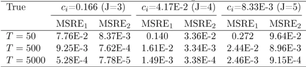
the accuracy of the estimation using methods (35) and (36), respectively. Table 1 displays the MSREs of the estimate forc1. As can be seen in

Ta-Table 1: MSRE of estimate using two methods

True ci=0.166 (J=3) ci=4.17E-2 (J=4) ci=8.33E-3 (J=5)

MSRE1 MSRE2 MSRE1 MSRE2 MSRE1 MSRE2

T = 50 7.76E-2 8.37E-3 0.140 3.36E-2 0.272 9.64E-2

T = 500 9.25E-3 7.62E-4 1.61E-2 3.34E-3 2.44E-2 8.96E-3

T = 5000 5.28E-4 7.78E-5 1.49E-3 3.38E-4 2.46E-3 9.15E-4

ble 1, the MSREs from method (36) MSRE2are much smaller than that from

method (35) MSRE1. This implies that method (36) needs a smaller sample

size of the Gibbs sampler to attain the same accuracy. Furthermore, it can be seen that the MSREs decreases as sample size increases, and small com-plexityci =8.33E-3 needs more sample size than large complexityci= 0.166

to obtain the same magnitude of MSREs. This implies we can determine sample sizeT for both methods (35) and (36) based on the acceptable

esti-mation accuracy and the size of the probability under estiesti-mation. This will be discussed in the next section.

5.5 Sample size determination for the Gibbs sampler

This section discusses the sample size T of the Gibbs sampler needed to

accurately estimateP(βk>0|β1 >0, . . . , βk−1 >0), which has a true value PT rue. As stated earlier, this probability is estimated using method (35)

if k > M, and method (36) if k ≤ M. For method (35), Hoijtink (2012,

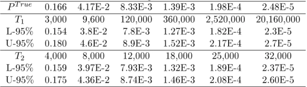
p.154) proposes a rule to determine the sample sizeT1 needed to accurately

estimate the complexity or t, which is shown in the top panel of Table 2. The criterion is that the95%central credibility interval for the estimate has

lower and upper bounds that are less than10%dierent from the true value.

The rst row in Table 2 displays the true probabilitiesPT ruethat needs to be

estimated. In addition, L-95%and U-95%demonstrate the lower and upper

bounds of the95%central credibility interval when using the corresponding

T1 above.

For method (36), we present a new rule to determine the sample sizeT2

based on a more strict accuracy criterion, that is, the dierences between both L-95% and U-95%, and PT rue are less than 5%. We let N(µβk, σ

2 βk) denote the distribution of βk in P(βk|β1 > 0, . . . , βk−1 > 0), where µβk is the mean andσ_β2

k is the variance. Then equation (36) becomes

P(βk|β1 >0, . . . , βk−1>0) = P(βk>0|βk∼N(µβk, σ

2 βk))

Table 2: Gibbs sample size determination

PT rue 0.166 4.17E-2 8.33E-3 1.39E-3 1.98E-4 2.48E-5 T1 3,000 9,600 120,000 360,000 2,520,000 20,160,000

L-95% 0.154 3.8E-2 7.8E-3 1.27E-3 1.82E-4 2.3E-5

U-95% 0.180 4.6E-2 8.9E-3 1.52E-3 2.17E-4 2.7E-5

T2 4,000 8,000 12,000 18,000 25,000 32,000

L-95% 0.159 3.97E-2 7.93E-3 1.32E-3 1.89E-4 2.37E-5

U-95% 0.175 4.36E-2 8.74E-3 1.46E-3 2.08E-4 2.60E-5

where_λˆ_k=µβ

k/σβk is the standardized population mean of βk. The princi-ple of the samprinci-ple size determination for method (36) is based on two facts. First, in the Gibbs sampler, we obtain T2 samples of βk from N(µβk, σ

2 βk) or standardizedβk fromN(ˆλk,1). This implies that the distribution of the

standardized sample mean of βk, denoted by λk, is N(ˆλk,_T1₂). Second, the

probabilityP(βk|β1 >0, . . . , βk−1 >0)is a one-to-one correspondence

func-tion of ˆ_{λk. For example, if λ}ˆ_{k = 0, we obtain a probability of 1/2, and}

conversely if the true value of the probability is1/6, we would expect aˆλk of

−0.97. These enable us to determine the sample sizeT2 needed to accurately

estimateP(βk>0|β1>0, . . . , βk−1 >0)given a true valuePT rue using the

following steps.

1. Compute_λˆ_{ksuch thatP(βk>0|βk∼N(ˆλk,1)) =P}T rue_{, and initialize} T2 = 1000.

2. Sample λk 10000 times from N(ˆλk,_T1₂), and then obtain 10000

esti-mates ofP(βk>0|βk∼N(ˆλk,1)).

3. Using 10000 estimates ofP(βk>0|βk∼N(ˆλk,1)), compute their95%

central credibility interval(L, U).

4. If either |L−PT rue_|

PT rue >5% or

|U−PT rue_|

PT rue >5%, then T2 =T2+ 1000and go to Step 2.

The bottom panel of Table 2 displays the sample sizeT2 and the resulting

L-95% and U-95%from the procedure above given correspondingPT rue.

In Bain, Table 2 is adopted to determine the sample size T1 and T2 of

the Gibbs sampler for estimating each decomposed complexity and t based on methods (35) and (36). Because T1 or T2 is large enough to accurately

be sucient to estimate a probability that is larger than this PT rue. We

estimateP(βk|β1 >0, . . . , βk−1 >0) with a starting sample sizeT1 = 3000

ifk > MorT2= 4000ifk≤M, and gradually resetT1 orT2 based on Table

2 until the estimate of the complexity or t is larger than the corresponding

PT rue. Note that if the estimate is still less than 2.48E-5 when using the

correspondingT1 or T2, we specify T1 = 100,000,000or T2 = 100,000. 5.6 Summary of the computation of the Bayes factor

This section summarizes the computation of the Bayes factor forHi against Hu, which is a ratio of the t and complexity. The following steps describe

how our program computes the complexity and t, and therefore the Bayes factor.

1. Transform θ intoβ using the procedure shown in Section 5.2. Then, we obtain(β¯,β˜)and M the rank ofRi.

2. Repeat Step (1), . . . ,(6) for k = 1, . . . , K to estimate each P(βk >

0|β1>0, . . . , βk−1 >0)for the decomposed complexitycik,ik−1 and t

fik,ik−1.

(1) Initialize the sample size of the Gibbs sampler as T2 = 4000 if

k≤M andT1= 3000 if k > M, and initialize β= 0.

(2) Repeat Step (a) or (b) fort= 1, . . . , T2+100iterations ifk≤M or

fort= 1, . . . , T1+ 100iterations if k > M, where100denotes the

rst100iterations, that is, a burn-in phase of the Gibbs sampler.

(a) If k ≤ M + 1, then dene a boundary (L, U) = (0,∞) for ¯

β1, . . . ,β¯k−1 and no boundary for β¯k, . . . ,β¯K. Thereafter,

se-quentially generate a sample of_β¯t

from the truncated distri-bution of (34) as previously described in Step (i) and (ii) in Section 5.3.

(b) If k > M + 1, then dene a boundary (L, U) for β¯1, . . . ,β¯M

using the linear relation between the_β¯_>0andβ˜_>0.

There-after, sequentially generate a sample of_β¯t

from the truncated distribution of (34) as previously described in Step (i) and (ii) in Section 5.3. Then a sample of _β˜t _{is obtained by means of}

its linear dependence on_β¯t

.

(3) Discard all the iterations for whicht≤100to account the burn-in

(4) Ifk≤M, compute the probabilityP(βk>0|β1>0, . . . , βk−1 >0) =T₂−1PT2+100 t=101 P(βk >0|βk∼N(µtβk,(σ 2 βk) t_{)) using method (36)} in Section 5.4.

(5) Ifk > M, compute the probabilityP(βk>0|β1>0, . . . , βk−1 >0)

=T₁−1PT1+100

t=101 I(βkt >0|β1t>0, . . . , βkt−1>0)using method (35)

in Section 5.4.

(6) If P(βk|β1 > 0, . . . , βk−1 > 0) obtained in Step (4) or (5) is less

than the reference value that corresponds to the currentT2 or T1

in Table 2, respectively, then reset T2 or T1 using the value of the

next column in the table and restart the procedure from Step (2). If not, the estimation ofP(βk|β1>0, . . . , βk−1 >0)is completed,

which renders the decomposed complexity cik,ik−1 or t fik,ik−1.

This was elaborated in Section 5.5.

3. The complexity and t can be computed by ci = QKk=1cik,ik−1 and

fi=QKk=1fik,ik−1 shown in Section 5.1. Then, the Bayes factor forHi

againstHu isBFiu=fi/ci.

6 Empirical applications in SEM

In this section, our procedure of evaluating order constrained hypotheses will be illustrated using two classic SEM applications. One example concerns conrmatory factor analysis (CFA), and the other example concerns multiple regression model.

6.1 Conrmatory factor analysis

In the rst example, we reanalyze a dataset built into lavaan called Holzinger-Swineford1939 (Rosseel, 2012). This dataset is taken from the Holzinger and Swineford 1939 (H&S) study, which is a commonly used example in factor analysis. The raw dataset consists of scores of 301 seventh and eighth grade students from the Pasteur School (n=145) and Grant-White School (n=156) who participated in 26 psychological aptitude tests. In our example, only a subset with 9 variables of the complete data is extracted to measure 3 correlated latent variables, each with three indicators, i.e.,

• a visual factor (ξ1) is measured by visual perception (x1), cubes (x2)

and lozenges (x3).

• a textual factor (ξ2) is measured by paragraph comprehension (x4),

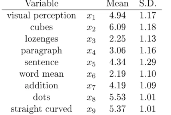
Table 3: Descriptives for the variables in the conrmatory factor analysis Variable Mean S.D. visual perception x1 4.94 1.17 cubes x2 6.09 1.18 lozenges x3 2.25 1.13 paragraph x4 3.06 1.16 sentence x5 4.34 1.29 word mean x6 2.19 1.10 addition x7 4.19 1.09 dots x8 5.53 1.01 straight curved x9 5.37 1.01

• a speed factor (ξ3) is measured by addition (x7), counting of dots (x8)

and discrimination of straight and curved capitals (x9).

The descriptives for the observed variables are given in Table 3, whereas the relations between latent variables and their indicators are formulated in the next paragraph and expressed using path notation (without showing measurement errors) in Figure 1.

The conrmatory factor analysis model for the H&S data can be repre-sented as:

x=Λxξ+x, (38)

wherex= (x1, . . . , x9)T denotes observed variables,ξ = (ξ1, ξ2, ξ3)T denotes

latent variables, ΛT_x =   θ1 θ2 θ3 0 0 0 0 0 0 0 0 0 θ4 θ5 θ6 0 0 0 0 0 0 0 0 0 θ7 θ8 θ9   (39)

is a matrix of factor loadings, andx is a3×1vector of measurement errors

with x ∼ N(0,Ψx) and Ψx being its covariance matrix. The covariance matrix of observed variables is given by:

Σx =ΛxΦξΛTx +Ψx, (40) where the factor covariance matrixΦξ is a symmetric matrix:

Φξ=   φ11 φ12 φ13 φ12 φ22 φ23 φ13 φ23 φ33  . (41)

visperc (𝑥𝑥₁) cubes (𝑥𝑥₂) lozenges (𝑥𝑥3) visual (𝜉𝜉₁) textual (𝜉𝜉₂) speed (𝜉𝜉₃) paragraph (𝑥𝑥4) sentence (𝑥𝑥₅) wordmean (𝑥𝑥₆) addition (𝑥𝑥7) dots (𝑥𝑥₈) straight curved (𝑥𝑥9)

Figure 1: Conrmatory factor analysis

Because the conrmatory factor analysis model is a measurement model without a structural model, we can simply specify this model using lavaan syntax in R (see Appendix A). To ensure that the target parameters are com-parable, we standardize them all. As is elaborated in Appendix A, lavaan provides both the standardized estimates and covariance matrix of target parameters. Recall that this is all the information that Bain needs to com-pute Bayes factors. Furthermore, in factor analysis models, indicators are required to both identify the model and set a metric for latent variables. This can be typically achieved either by standardizing the variances of la-tent variables or by constraining one factor loading per lala-tent variable to 1. In this example, the former way is chose.

Factor loadings indicate the degree of correspondence between the factor and the indicator, with higher loadings making the indicator more repre-sentative of the factor. Researchers might be interested in the issue which indicator plays the most important role in dening a factor. For instance, the rst indicator of every factor may be expected to be strongest, which can be represented by the following hypothesis

H1 :

θ1 >{θ2, θ3} θ4 >{θ5, θ6}

θ7 >{θ8, θ9}

We can also test a hypothesis with respect to the structure of the correlations between the latent variables. For example, we can evaluate whether the correlation between visual and textual is larger than the correlation either between visual and speed or between textual and speed:

H2 :φ12>{φ13, φ23}. (43)

Using R package Bain (the user manual of Bain can be found in Appendix B) to compute Bayes factors forH1 againstHuorH1c rendersBF1u = 0.076 or BF11c = 0.073. ForH2 againstHu or H2c, Bain renders BF2u = 1.33 or

BF22c = 1.59. These results imply that hypothesis H1 is not supported by the data, and the evidence from the data for H2 is not convincing because BF2u or BF22c is quite close to 1.

6.2 Multiple regression with latent variables

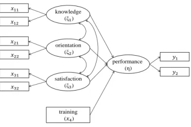
In a study reported by Warren, White, and Fuller (1974) (data available at https://informative-hypotheses.sites.uu.nl/software/bain), a sam-ple of 98 managers of farmer cooperatives was selected with the objective of studying managerial behavior. They postulated that a latent variable manager performance (η) was predicted by three correlated latent variables,

i.e., knowledge (ξ1), orientation (ξ2) and satisfaction (ξ3), and an observed

variable training (x4). The latent variablesη,ξ1,ξ2, andξ3 were measured

based on qualitative and quantitative answers to identical questionnaires collected from a random sample of managers in farmer cooperatives. These variables are assumed to be measured with error, and the errors of measure-ment were computed using the split halves procedure (Warren, et al., 1974) for all variables subject to measurement error:

• η is measured byy1 andy2,

• ξ1 is measured by x11 and x12,

• ξ2 is measured by x21 and x22,

• ξ3 is measured by x31 and x32.

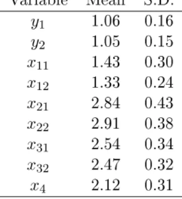
The observed variables are described in Table 4 and the graphical specica-tion of this structural equaspecica-tion model is found in Figure 2.

As can be seen from Figure 2, the relations of the variables can be repre-sented by a multiple regression model withη,ξ1,ξ2, and ξ3 that are latent.

Table 4: Descriptives for the variables in the multiple regression model Variable Mean S.D. y1 1.06 0.16 y2 1.05 0.15 x11 1.43 0.30 x12 1.33 0.24 x21 2.84 0.43 x22 2.91 0.38 x31 2.54 0.34 x32 2.47 0.32 x4 2.12 0.31

The measurement model is given by

y = Λyη+y

x = Λxξ+x, (44)

where x = (x11, x12, x21, x22, x31, x32)T denotes observed variables, and η

andξ = (ξ1, ξ2, ξ3)T are latent variables. For the structural model, we have η=θ0+θ1ξ1+θ2ξ2+θ3ξ3+θ4x4+δ, (45)

where θ0 is the intercept, θ1, θ2, θ3, and θ4 are regression coecients, and δ ∼ N(0, σ2) is the residual. This regression model is analyzed in lavaan

(see Appendix A). We standardize the coecients to make them comparable. Using the standardized estimates and covariance matrix of these coecients from lavaan, Bain can compute Bayes factors.

The hypothesis we evaluated is based on the results obtained by Warren et al. (1974) It states that knowledge is the strongest predictor followed by orientation, training and satisfaction. The resulting hypothesis is

H3:θ1 > θ2> θ4 > θ3. (46)

This hypothesis can be compared to, for example, knowledge is stronger than orientation followed by satisfaction and training:

H4:θ1 > θ2> θ3 > θ4, (47)

and training is stronger than satisfaction followed by orientation and knowl-edge:

𝑥11 𝑥12 𝑥21 𝑥22 knowledge (ξ1) 𝑥31 𝑥32 𝑦1 orientation (ξ2) satisfaction (ξ3) performance (η) 𝑦2 training (𝑥4)

Figure 2: Multiple regression with latent variables Table 5: Bayes factors and PMPs ofH3,H4 and H5

BFic PMPs H3 11.90 0.785 H4 2.676 0.214 H5 0.010 0.001

The results of the evaluation of these three hypotheses using Bain are dis-played in Table 5 (the user manual of Bain can be found in Appendix B). As can be seen, there is evidence in favor ofH3, no convincing evidence for H4, and evidence against H5. Furthermore, it can be seen from the PMPs

introduced in (15) thatH3 receives the largest support from the data.

7 Discussion

Order constrained hypotheses provide a representation of a researcher's the-ory with respect to the relations between the parameters of interest in SEM models. We developed a Bayes factor that can evaluate these hypotheses in a direct manner. A very vague prior was proposed that incorporates the covariance structure of the target parameters in the data. A proof was given that the prior probability that the order constraints hold, a key ingredient

of the Bayes factor when testing order constrained hypotheses, was invariant for linear transformations of the data.

The multivariate normal prior that is used to compute the prior proba-bility can be applied to order constrained testing problems where parame-ters have symmetric prior distributions such as regression coecients, group means, and factor loadings. Even in the case of non-symmetric prior distri-butions, the procedure will be accurate in most cases. For example, when testing a specic ordering of J variances using identical inverse gamma

pri-ors, the prior probability of this specic ordering will be equal to1/J!which

is identical to when computing the probability using independent normal pri-ors. The method could break down in asymmetric cases where the boundary value does not lie in the middle of a parameter space. For instance when testing0≤θ < .2 versus.2≤θ≤1, whereθ is the probability of a success

in a binomial experiment, and a uniform prior is specied on θ, the prior

probabilities of θ falling in these two intervals could be dierent than when

computing the probability using a normal distribution on θ. Extending the

methodology for such asymmetric testing problems would be an interesting topic to explore for future research.

Furthermore, a new algorithm was developed to ensure fast computa-tion to ensure general utilizacomputa-tion of the methodology by applied researchers. The methodology was implemented in the R package Bain which only needs the estimates and covariance matrix of target parameters (which can be ob-tained from the free R-package lavaan), and one or more restriction matrices representing a researcher's expectations. The output from Bain consists of Bayes factors and posterior probabilities for the hypotheses. These can be used which provide a direct answer about the relative evidence in the data between the hypotheses under investigation.

Appendix

A Estimates and covariance matrix obtained using

lavaan

Bain uses the estimates and covariance matrix of target parameters to com-pute Bayes factors. These can be obtained from the R package lavaan (Rosseel, 2012). This appendix illustrates how to obtain the estimates and covariance matrix of target parameters using the two examples discussed in

Section 6.

First of all, researchers need to install the version 0.5-18 or higher version of lavaan by starting R and typing install.packages("lavaan"). Note that R should be upgraded to R.3.5.0 or a higher version. The user manual of the latest version of lavaan can be found at

https://CRAN.R-project.org/package=lavaan.

The following R syntax renders the estimates and covariance matrix for the CFA model presented in Section 6.1.

# Load lavaan package. library(lavaan)

# Specify the CFA model.

CFA.model <- 'visual = x1 + x2 + x3 textual = x4 + x5 + x6 speed = x7 + x8 + x9'

fit<-cfa(CFA.model,data=HolzingerSwineford1939,std.lv = TRUE) # Obtain standardized estimates of parameters

standardizedSolution(fit)

# Obtain standardized covariance matrix of parameters. Sigma <- lavInspect(fit, "vcov.std.all")

Sigma[1:9,1:9] # For target parameters in (42) Sigma[19:21,19:21] # For target parameters in (43)

The output of standardizedSolution(fit, ci = FALSE) for the CFA model is lhs op rhs est.std se z pvalue 1 visual = x1 0.772 0.055 14.041 0 2 visual = x2 0.424 0.060 7.105 0 3 visual = x3 0.581 0.055 10.539 0 4 textual = x4 0.852 0.023 37.776 0 5 textual = x5 0.855 0.022 38.273 0 6 textual = x6 0.838 0.023 35.881 0 7 speed = x7 0.570 0.053 10.714 0 8 speed = x8 0.723 0.051 14.309 0 9 speed = x9 0.665 0.051 13.015 0 ... 22 visual textual 0.459 0.064 7.189 0 23 visual speed 0.471 0.073 6.461 0 24 textual speed 0.283 0.069 4.117 0

Note that the label visual = x1 denotes the factor loadingθ1 relating x1 to ξ1 and the label visual textual denotes the covariance φ12

be-tweenξ1 and ξ2. We only show the results for nine factor loadings used in

(42) and three covariances used in (43). The standardized estimates of the target parameters are given in the column under est.std. For example, the estimate ofθ4 is 0.852 in the row of textual = x4, and the estimate ofφ23

is 0.283 in the row of textual speed.

The output of Sigma contains the standardized covariance matrix of the target parameters. We only show the covariance matrix Sigma[19:21,19:21] ofφ12,φ13, andφ23:

visualtextual visualspeed textualspeed

visualtextual 0.0040678110 0.0007276616 0.001156340

visual speed 0.0007276616 0.0053037342 0.001480068

textual speed 0.0011563398 0.0014800678 0.004723718

The following R syntax renders the estimates and covariance matrix for the regression model in Section 6.2.

# Load lavaan package. library(lavaan)

# Set R working director where the data is saved. setwd("C:/Example2")

# Read data "performance.csv".

performance<-read.csv("performance.csv") # Specify the regression model.

perform.model<-' # measurement model kno = x11 + x12 ori = x21 + x22 sat = x31 + x32 per = y1 + y2 # regressions

per kno + ori + sat + tra'

fit<-sem(perform.model,data=performance,std.lv = TRUE) # Obtain standardized estimates and covariance matrix

standardizedSolution(fit)

Sigma[9:12,9:12] # For target parameters in (46), (47), (48) The output of standardizedSolution(fit, ci = FALSE) for the re-gression model is lhs op rhs est.std se z pvalue ... 9 per kno 0.478 0.161 2.960 0.003 10 per ori 0.336 0.165 2.030 0.042 11 per sat 0.151 0.105 1.440 0.150 12 per tra 0.286 0.084 3.403 0.001 ...

Note that the label per kno denotes the coecient θ1 which relates η to ξ1 in the regression model (45). We only show the results for the

four regression coecients used in (46), (47), and (48). The standardized estimates of the target parameters are given in the column under est.std. For example, the estimate of θ1 is 0.478 in the row of per kno, and the

estimate ofθ4 is 0.286 in the row of per tra.

The output of Sigma[9:12,9:12] renders the standardized covariance matrix ofθ1, . . . , θ4:

perkno perori persat pertra

perkno 0.026034895 -0.0223249106 -0.0050273595 -0.0011610045 perori -0.022324911 0.0273346337 0.0043904540 -0.0007619234 persat -0.005027359 0.0043904540 0.0110250662 -0.0002713825 pertra -0.001161004 -0.0007619234 -0.0002713825 0.0070519650

The standardized estimates and covariance matrix of target parameters obtained in lavaan can be used as input for Bain. This will be shown in the user manual in Appendix B.

B User Manual of Bain

Bain is an R package developed for the evaluation of order constrained hy-potheses using the algorithm presented in the paper. It can be downloaded at https://informative-hypotheses.sites.uu.nl/software/bain/. Windows, Mac, and Linux versions are oered, respectively, by downloaded les Bain_xxx.zip, Bain_xxx.tgz, and Bain_xxx.tar.gz, where xxx denotes package version. After downloading the package, for example, windows users can install Bain in R by