Title
Interacting Default Intensity with a Hidden Markov Process
Author(s)
YU, F; Ching, WK; GU, J; SIU, TK
Citation
Quantitative Finance , 2017, v. 17, p. 781-794
Issued Date
2017
URL
http://hdl.handle.net/10722/240945
Rights
Postprint:
This is an Accepted Manuscript of an article published by Taylor
& Francis Group in [Quantitative Finance] on [2017], available
online at:
http://www.tandfonline.com/doi/abs/10.1080/14697688.2016.1237
036; This work is licensed under a Creative Commons
Attribution-NonCommercial-NoDerivatives 4.0 International
License.
arXiv:1603.02902v1 [q-fin.CP] 9 Mar 2016
Interacting Default Intensity with Hidden Markov
Process
Feng-Hui Yu ∗ Wai-Ki Ching † Jia-Wen Gu ‡ Tak-Kuen Siu §
March 10, 2016
Abstract
In this paper we consider a reduced-form intensity-based credit risk model with a hidden Markov state process. A filtering method is proposed for extracting the underlying state given the observation processes. The method may be applied to a wide range of problems. Based on this model, we derive the joint distribution of multiple default times without imposing stringent assumptions on the form of default intensities. Closed-form formulas for the distribution of default times are obtained which are then applied to solve a number of practical problems such as hedging and pricing credit derivatives. The method and numerical algorithms presented may be applicable to various forms of default intensities.
Keywords: Reduced-form Intensity Model; Default Risk; Credit Derivatives; Hidden Markov Model (HMM).
1
Introduction
Modeling credit risk has long been a critical issue in credit risk management. Attention has been given to it especially since the global financial crisis in 2008. Credit risk modeling has a lot of applications, for example, pricing and hedging the credit derivatives, as well as the management of credit portfolios. Models adopted in the finance industry may be grouped into two major
∗Advanced Modeling and Applied Computing Laboratory, Department of Mathematics, The University of
Hong Kong, Pokfulam Road, Hong Kong. E-mail: [email protected].
†Corresponding author. Advanced Modeling and Applied Computing Laboratory, Department of Mathematics,
The University of Hong Kong, Pokfulam Road, Hong Kong. E-mail: [email protected].
‡Department of Mathematical Science, University of Copenhagen, Denmark. E-mail: [email protected]. §Department of Applied Finance and Actuarial Studies, Faculty of Business and Economics, Macquarie
categories: structural firm value models and reduced-form intensity-based models. For the first class of models, it was pioneered by Black and Scholes (1973) and Merton (1974). The key idea of the structural firm’s value model is to model the default of a firm by using its asset value, where the asset value is governed by a geometric Brownian motion. When the asset value falls below a certain prescribed level, the default of the firm is triggered. For the second kind of model, it was pioneered by Jarrow and Turnbull (1995) and Madan and Unal (1998). The main idea of reduced-form intensity-based models is to consider the defaults as exogenous processes and describe their occurrences with Poisson processes and their variants.
The interacting intensity-based default models are widely adopted to model the portfolio credit risk and defaults. Since we focus on contagion models in this paper as in, for example, Giesecke (2008), we differentiate intensity-based credit risk models into top-down models and bottom-up models. The top-down models focus on modeling the default times at the portfolio level without reference to the intensities of individual entities. Based on this, one can also recover the individual entity’s intensity with some method like random thinning, etc. Some works related to this class of models include Davis and Lo (2001), Giesecke, Goldberg and Ding (2005), Brigo, Pallavicini and Torresetti (2006), Longstaff and Rajan (2008) and Cont and Minca (2011), etc. While the bottom-up model focuses on modeling the default intensities of individual reference entities and their aggregation to form a portfolio default intensity. Some works related to this class of models include Duffie and Garleanu (2001), Jarrow and Yu (2001), Sch¨onbucher and Schubert (2001), Giesecke and Goldberg (2004), Duffle et al. (2006) and Yu (2007), etc. The differences between these two classes of models are the form of individual entity’s default intensities and the way the portfolio aggregation is formed. In this paper we shall focus on a bottom-up model.
Based on the model developed by Lando (1998), Yu (2007) extended the model and applied the extended model multiple defaults and their correlation. In addition, Yu adopted the total hazard construction method proposed by Norros (1986) and Shaked and Shathanthikumar (1987) to simulate the distribution of default times which have interacting intensities. Zheng and Jiang (2009) then adopted this method and derived closed-form formulas for the multiple default distributions under their contagion model. Gu et al. (2013) introduced a recursive method to calculate the distribution of ordered default times, and Gu et al. (2014) further proposed a hidden Markov reduced-form model with a specific form of default intensities.
In this paper we develop a generalized reduced-form intensity-based credit model with hidden Markov process. The model is applicable to a wide class of default intensities with various forms
of dependent constructions. For the hidden Markov process, we also discuss a flexible method to extract the hidden state process given the observations processes, which may hopefully have applications in diverse fields. Then using the total hazard construction method by Yu (2007), we derive closed-form formulas for the joint default distribution. When the intensities are homogeneous, analytic algorithm for the calculation of the joint distribution of ordered default times is provided. The explicit formula may enhance the computational efficiency in applications, for instance, pricing of credit derivatives. We remark that the results in Gu et al. (2014) is a special case of the method discussed here. In addition, we extend the total hazard construction method to the cases with hidden process to simulate the joint distribution of default times. We remark that hidden Markov models have been employed in studying credit risk, see for instance, Frey and Runggaldier (2010, 2011), Frey and Schmidt (2011), Elliott and Siu (2013) and Elliott et al. (2014).
The rest of this paper is structured as follows. Section 2 gives a snapshot of the interacting intensity-based default model with hidden Markov process. Section 3 presents the method for extracting the hidden state process from the observation processes. Section 4 derives the closed-form expression for the joint default distribution based on the total hazard construction method, and also presents an analytic formula for the distribution of ordered default times. Besides, the extended total hazard construction method under a hidden Markov process to obtain the joint distribution of default times is also presented. Section 5 provides numerical methods for some situation in Section 3 which may be used in both Sections 3 and 4, and error analysis is also discussed. Section 6 illustrates an application of the proposed method in pricing credit derivatives. Finally, Section 7 concludes the paper.
2
Model Setup
Let (Ω,F, P) be a complete probability space where P is a risk-neutral probability measure, which is assumed to exist. Suppose there are K interacting entities, and we let Ni(t) :=
1{τi≤t}, where τi is a stopping time, representing the default time of credit name i, for each
i= 1,2,· · ·, K. Suppose we have an underlying state process (Xt)t≥0 describing the dynamics
of the economic condition. Let FX
t := σ(Xs,0 ≤ s ≤ t)∨ N where N represents all the null
subsets of Ω in F and C1∨ C2 is the minimalσ-algebra containing both the σ-algebras C1 and
C2. We also letHt:=σ(Xt)∨ FtN where
FN
We assume that for eachi= 1,2, . . . , K,Ni(t) possesses a nonnegative, {Ht}t≥0-adapted,
inten-sity processλi satisfying
E Z t 0 λi(s)ds <∞, t≥0, (1)
such that the compensated process
Mi(t) :=Ni(t)− Z t∧τi
0
λi(s)ds , t≥0, (2)
is an ({Ht}t≥0, P)-martingale. Note that after the default timeτi, Ni(t) will stay at the value
one, so there is no need to compensate for Ni(t) after time τi, see, for example, Elliott et al.
(2000).
For all the market participants, we assume that they cannot observe the underlying process (Xt)t≥0 directly. Instead, they observe the process (Yt)t≥0, revealing the delayed and noisy
information of (Xt)t≥0, and also observe the default process (Nti)t≥0. Hence, the common
information set available to the market participants at time t is Ft :=FtY ∨ FtN whereFtY :=
σ(Ys,0≤s≤t)∨ N. We further assume that (Xt)t≥0 is an “exogenous” process to (Nti)t≥0, i=
1,2, . . . , K, i.e., For anyt, theσ-fieldsFX
∞ andFtN are conditionally independent givenFtX and
P(τi 6=τj) = 1, i6=j.
To simplify our discussion, throughout the paper, we suppose that (Xt)t≥0 is a two-state
Markov chain taking a value in {x0, x1}. We assume the transition rates of the chain for
“x0 → x1” and “x1 → x0” are θ0 and θ1, respectively. The observable process (Yt)t≥0 is
again a two-state Markov chain taking value in{y0, y1}, with transition rates depending onXt,
i.e., η0(Xt)(y0 → y1) and η1(Xt)(y1 →y0), where η0 and η1 are real-valued functions. At time
0, we suppose that X0 is in state x0 and Y0 is in state y0. The methods introduced later in
our paper may still be applicable when the Markov chainsX andY have more than two states though more complicated notation may involve.
3
Extraction of Hidden State Process with Observable
Pro-cesses
To specify the form of the intensities, we give the following notations. Suppose that at time t, NtD defaults have already occurred at t1, t2, . . . , tND
t such that 0 =t0< t1<· · ·< tND t ≤t. Then we denote TND t = (t1,· · ·, tNtD) the ordered N D
t default times and IND
t = (j1,· · ·, jNtD)
assume that i > ND
t and t < τi, where τi is the obligor i’s default time. Each process λi
(i = 1, . . . , K), is {Ht}t≥0-predictable, that is to say λi(t) is known given information about
the chain X and all the default processes prior to time t. Then the intensity of τi may be
written as λit = λi(t|IND
t , TNtD, Xt) where Xt is the state of chain X at time t. Note that
(IND
t , TNtD, Xt)∈ Ht.
Since the path ofX is unobservable, while the path ofY and Ni, (i= 1, . . . , K) are
observ-able, we can use the relationship between X, Y and Ni, (i= 1, . . . , K) to find the probability
law ofX. We apply the recursive method proposed in Gu et al. [15] to calculate the conditional probability P(Xt=xi|Ft), (i= 0,1, t ≥0). Before discussing the method, we need to find the
expressions for all the unknown items in the recursive formulas. In the process of finding the expressions, we also present moment generating function method to achieve our goal.
3.1 Some Preliminaries
Let ¯Ti,k,j(s0,∆s) be the union of subintervals of time of the chain X in state xk in the time
interval [s0, s0+ ∆s] given the chain starts from Xs0 =xi and ends at Xs0+∆s =xj. For each
i, j= 0,1, we let ¯
Ti,j(s0, t) = ( ¯Ti,0,j(s0, t),T¯i,1,j(s0, t))T and u(¯t) = (u0(¯t), u1(¯t))T
where ¯t ∈ [s0, s0+t]. Note that ¯Ti,1,j(s0, t) = [s0, s0 +t]\T¯i,0,j(s0, t). Since jumps in chain Y
and defaults are Poisson processes, using the concept of moment generating function, we define ¯ Ψij(s0,u, t) =E " exp (Z ¯ Ti,0,j(s0,t) u0(¯t)d¯t+ Z ¯ Ti,1,j(s0,t) u1(¯t)d¯t )# .
Note that u(¯t) is an arbitrary integrable function. This means, in this case, we can adopt this moment generating function. For instance,u(¯t) can be the transition rates of jumps in chainY or the default rates which are the default intensities accumulated by all the entities by time ¯t before default.
Proposition 1 Let Φ¯ij(s0,u, t) =Pij(t) ¯Ψij(s0,u, t), where Pij(t) is the probability that a
pro-cess in state xi will be in state xj after a time of t, and i, j= 0,1. Then ¯ Φij(s0,u, t) =θi Z t 0 exp Z s0+t−s s0 (ui(¯t)−θi)d¯t ¯ Φjj(s0+t−s,u, s)ds ¯ Φii(s0,u, t) =θi Z t 0 exp Z s0+t−s s0 (ui(¯t)−θi)d¯t ¯ Φji(s0+t−s,u, s)ds+ exp Z s0+t s0 (ui(¯t)−θi)d¯t (3) where i, j= 0,1.
Proof: ¯ Ψij(s0,u, t) = E " exp Z ¯ Ti,0,j(s0,t) u0(¯t)d¯t+ Z ¯ Ti,1,j(s0,t) u1(¯t)d¯t !# = θi Pij(t) Z t 0 e−θis·e Rs0+s s0 ui(¯t)dt¯P jj(t−s)E " exp Z ¯ Tj,0,j(s0+s,t−s) u0(¯t)d¯t+ Z ¯ Tj,1,j(s0+s,t−s) u1(¯t)d¯t !# ds = θi Pij(t) Z t 0 exp Z s0+s s0 (ui(¯t)−θi)d¯t Pjj(t−s) ¯Ψjj(s0+s,u, t−s)ds = θi Pij(t) Z t 0 exp Z s0+t−s s0 (ui(¯t)−θi)d¯t Pjj(s) ¯Ψjj(s0+t−s,u, s)ds. We also have ¯ Ψii(s0,u, t) = θi Pii(t) Z t 0 e Rs0+t−s s0 (ui(¯t)−θi)d¯tP ji(s) ¯Ψji(s0+t−s,u, s)ds+ e Rs0+t s0 (ui(¯t)−θi)d¯t Pii(t) . Replace ¯Ψij(s0,u, t) by ¯ Φij(s0,u,t)
Pij(t) , we can then get the system of equations in the proposition.
We find that when the expression of u(¯t) satisfies some “good” property, Eq. (3) in the above proposition has a unique solution. The property is that u(¯t) does not have any direct relationship with time ¯teven though it may have implied relationship with ¯t. This meansu(¯t) can be written as u. Then, not only the problem of solving Eq. (3) can be simplified, but some related definitions can also be simplified as well. Similar as before, let Ti,k,j(∆s) be the
occupation time of the chainXin statexkin the time interval [s, s+∆s] given the chain starting
from Xs=xi and ending atXs+∆s=xj. For each i, j = 0,1, we let
Ti,j(t) = (Ti,0,j(t), Ti,1,j(t))T and u= (u0, u1)T ∈R2.
The moment generating function of Ti,j(t) is given by
Ψij(u, t) =E(exp{uTTi,j(t)}).
Apply the same method to Ψij(u, t) as we have done to ¯Ψij(u, t), and let
Φij(u, t) = Ψij(u, t)·Pij(t).
We can also get the equivalent Eq. (3) for Φij(u, t), i.e., replacing ¯Φij(u, t) with Φij(u, t),
(ui(¯t)−θi) with ui−θi in Eq. (3). Then to solve the equivalent equation, it suffices to solve a
linear system of O.D.E.s (c.f. Gu et al. [15]): ∂Φ(u, t)
where Φ(u, t) = Φ11(u, t) Φ12(u, t) Φ21(u, t) Φ22(u, t) and A= u0−θ0 θ0 θ1 u1−θ1 .
This linear system of O.D.E.s is known as the fundamental matrix equation in the literature. Then it is well-known that the equation has a unique solution which is called the fundamental matrix solution with the initial condition Φij(u,0) = 1, i, j= 0,1 as
Φ(u, t) =eAt1·1T
where 1 is the two-dimensional column vector with all entries being equal to 1. Hence we can get the solution for Ψij(u, t) by
Ψij(u, t) =
Φij(u, t)
Pij(t)
.
In practice, when the expressions of ui(¯t), (i= 0,1) are given, we can substitute them into
the above Eq. (3), then intuitively we can check whether it has a solution. Note that the expressions of ui(¯t), (i= 0,1) determine whether the system is solvable. If it is solvable, then
we can obtain the solution ¯Φij(s0,u, t), (i, j= 0,1). Note that the results in [15] can be regarded
as a special case that has a unique solution.
3.2 Recursive Formulas for Extracting Hidden Process
Forωet∈ Ft, we can expressωet in a more clear way as follows:
e ωt= (NtY, NtD, SNY t , INtD, TNtD) where • SNY t = (s1, s2, . . . , sNtY), • IND t = (j1, j2, . . . , jNtD), • TND t = (t1, t2, . . . , tNtD), • NY
t counts the number of jumps in chain Y by time t,
• ND
t counts the number of defaults by timet,
• (s1, s2, . . . , sNY
t ) is the collection of ordered jump times of the chain Y by time t, i.e.,
0< s1< . . . < sNY t ≤t,
• (t1, t2, . . . , tND
t ) is the collection of ordered default times by time t, i.e., 0 < t1 < . . . <
tNY t ≤t,
• (j1, j2, . . . , jND
t ) is the collection of ordered corresponding name of defaulters by time t,
i.e., name ji defaults at time ti.
Hereωetcan be interpreted as the state of the stochastic dynamical system at timet. Given the
information up to time t, i.e., Ft, we divide the time period [0, t] into (NtY +NtD) sub-periods,
[0, h1], (h1, h2], . . . , (hNY
t +NtD−1, hNtY+NtD]. In each of them, exactly one default or one jump
in Y is observed. When there is no default or jump occurred by time t, the calculation of P(Xt=xi | Ft) can be simplified and we shall introduce it later.
Define ¯IND
t = (1,2, . . . , K)\INtD. Suppose that s and s+ ∆s are two endpoints of one
sub-period. The following characterizes the computational method for P(Xt = xi | Ft). For e ω∈ {tk=s+ ¯tk∈(s, s+ ∆s]}, P(Xs =xi | Fs+∆s) = P(Xs =xi | Fs, tk =s+ ¯tk, jk=β) = P(Xs=xi| Fs)·Pl=0,1fti,lk(s+ ¯tk;β, s,∆s) P j=0,1P(Xs=xj | Fs)·Pl=0,1f j,l tk(s+ ¯tk;β, s,∆s) (4) and P(Xs+∆s=xi| Fs+∆s) = X j=0,1 P(Xs =xj | Fs+∆s)P(Xs+∆s=xi | Fs+∆s, Xs=xj) = X j=0,1 P(Xs =xj | Fs+∆s) ftj,i k(s+ ¯tk;β, s,∆s) P l=0,1f j,l tk(s+ ¯tk;β, s,∆s) (5) where ftj,i k(t;β, s,∆s)dt=P(tk∈dt, jk =β, Xs+∆s =xi |Xs =xj, N D s , NsY, IND s ).
Similarly, we have for ωe∈ {sk =s+ ¯sk∈(s, s+ ∆s]},
P(Xs =xi | Fs+∆s) = P(Xs=xi | Fs)Pl=0,1f i,l sk(s+ ¯sk;s,∆s X j=0,1 P(Xs=xj | Fs) X l=0,1 fskj,l(s+ ¯sk;s,∆s (6) and P(Xs+∆s=xi | Fs+∆s) = X j=0,1 P(Xs=xj | Fs+∆s) fskj,i(s+ ¯sk;s,∆s) P l=0,1f j,l sk(s+ ¯sk;s,∆s (7) where fskj,i(t;s,∆s)dt = P(sk∈dt, Xs+∆s=xi |Xs=xj, NsD, NsY, IND s ).
Combining Eqs. (4), (5), (6) and (7), we obtain a recursive method for computing P(Xt =
xi | Ft) in terms of ftkj,i(s+ ¯tk;β, s,∆s) and fskj,i(s+ ¯sk;s,∆s). That is to say, with the fact
that P(X0 = x0|F0) = 1 and P(X0 = x1|F0) = 0, we can apply them to Eq. (4) or Eq. (6)
according to Ft, and then to get P(X0 = xi|F∆s) which are unknown in the calculation of
P(X∆s =xi|F∆s) in Eq. (5) or Eq. (7). The equation to calculateP(X∆s=xi|F∆s) should be
chosen according toFtas well. By repeating this recursion procedure, we can obtain the desired
conditional probabilities.
To get the expressions for the desired ftj,i
k(s+ ¯tk;β, s,∆s) and f j,i
sk(s+ ¯sk;s,∆s), we need
to use the method introduced in section 3.1. Replace u by −(ηi(x0), ηi(x1)), i = 0,1 and we
know that there exists unique solutions for Ψij, i, j = 0,1. Replace u(¯t) by −(λi(x0), λi(x1)),
i= 1,· · ·, K in Eq. (3), we then could have a direct sense of whether it is solvable or not. If it is solvable and has an analytical solution, then from the definition of ftj,i
k(s+ ¯tk;β, s,∆s) and fskj,i(s+ ¯sk;s,∆s), we get fj,i sk(s+ ¯sk;s,∆s) = X l=0,1 Pjl(¯sk)Pli(∆s−s¯k)ηC(NY s)(xl) ×Ψjl −(ηC(NY s)(x0), ηC(NsY)(x1)) T,¯s k ×Ψli −(ηC(NY s+1)(x0), ηC(NsY+1)(x1)) T,∆s−s¯ k ×Ψ¯jl s,− X i∈I¯N D s (λi(¯t|IND s , TNsD, x0), λi(¯t|INsD, TNsD, x1)) T,¯s k ×Ψ¯li s+ ¯sk,− X i∈I¯N D s (λi(¯t|IND s , TNsD, x0), λi(¯t|INsD, TNsD, x1)) T,∆s−¯s k , ftj,ik(s+ ¯tk;β, s,∆s) = X l=0,1 Pjl(¯tk)Pli(∆s−¯tk)λβ(s+ ¯tk|IND s , TNsD, Xs=xl) ×Ψjl(−(ηC(NY s)(x0), ηC(NsY)(x1)) T,¯t k) ×Ψli −(ηC(NY s)(x0), ηC(NsY)(x1)) T,∆s−¯t k ×Ψ¯jl s,− X i∈I¯ N Ds (λi(¯t|IND s , TNsD, x0), λi(¯t|INsD, TNsD, x1)) T,¯t k ×Ψ¯li s+ ¯tk,−Pi∈I¯∗ N Ds (λi(¯t|IN∗D s , T ∗ ND s , x0), λi(¯t|I ∗ ND s , T ∗ ND s , x1)) T,∆s−t¯ k whereIN∗D s =IN D s S {β}, TN∗D s =TN D s S {tβ} and C(x) = 1, x+Y0≡0 (mod 2) 0, x+Y0≡1 (mod 2).
If up to time t, no jump or default has been observed, then we have the following: forωe∈ {no jump or default observed in [0, t]},
P(Xt=xi | Ft) =
P(Xt=xi,no jump or default in[0, t]) X
j=0,1
P(Xt=xj,no jump or default in[0, t])
where
P(Xt=xj,no jump or default in[0, t]) = P(Xt=xj)Ψ0j −(ηC(0)(x0), ηC(0)(x1))T, t
×Ψ¯0j(0,
−Pi∈I(λi(¯t|IND
0 , TN0D, x0), λi(¯t|IN0D, TN0D, x1))
T, t).
Note that if the jump intensities of chain Y: ηi (i = 0,1), are not as simple as in our
as-sumptions and they are also related with time directly, i.e., ηi(¯t), all the algorithms
intro-duced above are still applicable and we just need to replace Ψij −(ηC(0)(x0), ηC(0)(x1))T, t by
¯
Ψij −(ηC(0)(x0), ηC(0)(x1))T, t
, i, j = 0,1. This replacement holds only when Eq. (3) given
u(¯t) =−(η0(¯t), η1(¯t)) has an analytical solution.
If Eq. (3) does not admit an analytical solution given ui(¯t), (i = 0,1), we also provide
numerical method in Section 5. Now we know how to getP(Xt=xi|Ft).
4
Default Distributions
We derive the default distributions in this section. Besides deriving closed-form expressions for default distributions, extended total hazard construction method for hidden Markov model to derive the joint default distribution is also presented.
4.1 Closed-Form Expressions for Default Distributions
In this subsection, we compute the conditional joint distribution of default times P(τ1> t1, τ2 > t2, . . . , τK > tK | Ft)
and the distribution of ordered default times
P(τk > s| Ft), k= 1,2, . . . , K.
Notice that whent= 0, we don’t have any information, the above two conditional probabilities become unconditional probabilities. As for the first probability, due to the Markov property of Xt and the structure of λi(t), we have
P(τ1> t1, τ2 > t2, . . . , τK > tK | F t)
= X
i=0,1
Since we know how to calculate P(Xt=xi| Ft), we only need to compute the conditional joint
probability P(τ1> t1, τ2 > t2, . . . , τK > tK | FN
t , Xt=xi).
Assume we first enter the market immediately after the NtDth default of the K obligors at time t, to simplify the notations, we denote m = ND
t , that means we already know the
information Tm = (t1,· · ·, tm), Im = (j1,· · ·, jm) and FtY by time t. Then we can get the
following equation:
P(τ1> t1, τ2 > t2, . . . , τK > tK | FN
t , Xt=xi)
= P(τjm+1 > tjm+1, . . . , τjK > tjK |τj1 =t
1, . . . , τjm =tm, Xt=xi).
Furthermore, we also know the relationship that f(tjm+1, . . . , tjK | F t) = (−1)K−m dK−m dtjm+1. . . dtKP(τ 1> t1, τ2 > t2, . . . , τK > tK | FN t , Xt=xi) where f(tjm+1, . . . , tjK | F
t) is the conditional joint density function. Therefore, to obtain the
desired conditional probability, it suffices to find its conditional joint density function.
Here we employ the approach introduced by Yu (2007) [27] (called the total hazard construc-tion method) to derive the condiconstruc-tional density funcconstruc-tion.
Proposition 2 The expression of the density function that we intend to get is in the form of expectation f(tjm+1, . . . , tjK | F t) =E K X l=m+1 X i∈I¯l λi(tjl|Il, Tl, Xtjl)·exp − K X l=m+1 (X i∈I¯l Z tjl tl λi(u|Il, Tl, Xu)du) .
Proof: Without loss of generality, we assume that tjm+1 < . . . < tjK. In this case, τm+1−τm
would be the first default time we observed after entering the market. By using the total hazard construction method pioneered by Yu (2007) [27] with the information already known, we draw a collection of independent standard exponential random variables: (Ejm+1,· · ·, EjK). Then we
know τm+1−τm = min i∈Im¯ Λ −1 i (Ei) = min i∈Im¯ inf{s≥0 : Λi(s)≥Ei}
which implies that
P τm+1−τm> t| Fτm=P min i∈Im¯ inf{ s≥0 : Λi(s)≥Ei}> t .
Suppose the information FX ∞ is known, then P(τm+1−τm > t| Fτm) = Y i∈Im¯ P Ei > Z tm+t tm λi(u|Im, Tm, Xu)du = Y i∈Im¯ exp − Z tm+t tm λi(u|Im, Tm, Xu)du = exp −X i∈Im¯ Z tm+t tm λi(u|Im, Tm, Xu)du .
Then if we assume that τm < t < τm+1 and ti > τi, i= 1, . . . , m, and let λm+1(t) denote the (m+ 1)th default rate at timet, then
λm+1(t) = X i∈Im¯ Z t tm λi(u|Im, Tm, Xu)du. Since P(τm+1 > t| Fτm, Xs(tm<s<∞)) =e− P i∈Im¯ Rt tmλi(u|Im,Tm,Xu)du=e−λm+1(t) we have P(τjm+1 > tjm+1, . . . , τjK > tjK | F t, Xs(tm<s<∞)) = K Y l=m+1 P(τjl > tjl | Ft, Xs(tm<s<∞)) = K Y l=m+1 e−λl(tjl) = K Y l=m+1 exp − X i∈Il¯−1 Z tjl tl−1 λi(u|Il−1, Tl−1, Xu)du = exp − K X l=m+1 ( X i∈Il¯−1 Z tjl tl−1 λi(u|Il−1, Tl−1, Xu)du) and therefore f(tjm+1, . . . , tjK | F t, Xs(tm<s<∞)) = (−1)K−m d K−m dtjm+1. . . dtKP(τ jm+1 > tjm+1, . . . , τjK > tjK | F t, Xs(tm<s<∞)) = (−1)K−m d K−m dtjm+1. . . dtK exp − K X l=m+1 ( X i∈Il¯−1 Z tjl tl−1 λi(u|Il−1, Tl−1, Xu)du) |tl −1=tjl−1 = K Y l=m+1 X i∈Il¯−1 λi(tjl|Il−1, Tl−1, Xtjl)·exp − K X l=m+1 ( X i∈Il¯−1 Z tjl tjl−1 λi(u|Il−1, Tl−1, Xu)du) and f(tjm+1, . . . , tjK | F t) =E[f(tjm+1, . . . , tjK | Ft, Xs(tm<s<∞))]
= E K Y l=m+1 X i∈I¯l−1 λi(tjl|Il−1, Tl−1, Xtjl)·exp − K X l=m+1 ( X i∈I¯l−1 Z tjl tjl−1 λi(u|Il−1, Tl−1, Xu)du) = E K Y l=m+1 X i∈Il¯−1 λi(tjl|Il−1, Tl−1, Xtjl)·exp − K X l=m+1 ( Z tjl tjl−1 X i∈Il¯−1 λi(u|Il−1, Tl−1, Xu)du) .
If Eq. (3) in the previous section given u(¯t) = −(λi(x0), λi(x1)), i = 1, . . . , K, has unique
solutions, then we further have the following result.
Proposition 3 The explicit formula for calculating the desired density function is in this form: f(tjm+1, . . . , tjK | F t) = (−1)K−m· X lm+1=0,1 X lm+2=0,1 · · · X lK=0,1 · d( ¯Ψilm+1(t jm,−P i∈Im¯ (λi(¯t|Im, Tm, x0), λi(¯t|Im, Tm, x1))T, tjm+1 −tjm)) dtjm+1 · d( ¯Ψlm+1lm+2(t jm+1,−P i∈Im¯ +1(λi(¯t|Im+1, Tm+1, x0), λi(¯t|Im+1, Tm+1, x1)) T, tjm+2−tjm+1)) dtjm+2 · · · · ·d( ¯ΨlK−1lK(t jK−1,−P i∈IK¯ −1(λi(¯t|IK−1, TK−1, x0), λi(¯t|IK−1, TK−1, x1)) T, tjK −tjK−1)) dtjK
where Ψ¯ij, i, j= 0,1 are the moment generating function defined in Section 3.
Proof: We note that
E K Y l=m+1 X i∈I¯l−1 λi(tjl|Il−1, Tl−1, Xtjl)·e −PK l=m+1( Rtjl tjl−1 P i∈Il¯ −1λi(u|Il−1,Tl−1,Xu)du) = X lm+1=0,1 X lm+2=0,1 · · · X lK=0,1 E X i∈I¯m λi(tjm+1|Im, Tm, Xtjm+1)·e Rtjm+1 tjm P i∈Im¯ λi(u|Im,Tm,Xu)du|X tjm =i, Xtjm+1 =lm+1 · E X i∈I¯m+1 λi(tjm+2|Im+1, Tm+1, Xtjm+2)·e Rtjm+2 tjm+1 P i∈Im¯ +1λi(u|Im+1,Tm+1,Xu)du|X tjm+1 =lm+1, Xtjm+2 =lm+2 · · · · ·E X i∈I¯K−1 λi(tjK|IK−1, TK−1, XtjK)·e RtjK tjK−1 P i∈IK¯ −1λi(u|IK−1,TK−1,Xu)du|X tjK−1 =lK−1, XtjK =lK = (−1)K−m· X lm+1=0,1 X lm+2=0,1 · · · X lK=0,1 d E eRt jm+1 tjm P i∈Im¯ λi(u|Im,Tm,Xu)du|X tjm =i, Xtjm+1 =lm+1 dtjm+1 · d E e Rtjm+2 tjm+1 P i∈Im¯ +1λi(u|Im+1,Tm+1,Xu)du|X tjm+1 =lm+1, Xtjm+2 =lm+2 dtjm+2 · · · · · d E e RtjK tjK−1 P i∈IK¯ −1λi(u|IK−1,TK−1,Xu)du|X tjK−1 =lK−1, XtjK =lK dtjK
= (−1)K−m· X lm+1=0,1 X lm+2=0,1 · · · X lK=0,1 d( ¯Ψilm+1(t jm,−P i∈I¯m(λi(¯t|Im, Tm, x0), λi(¯t|Im, Tm, x1)) T, tjm+1−tjm)) dtjm+1 · d( ¯Ψlm+1lm+2(t jm+1,−P i∈I¯m+1(λi(¯t|Im+1, Tm+1, x0), λi(¯t|Im+1, Tm+1, x1)) T, tjm+2−tjm+1)) dtjm+2 · · · · ·d( ¯ΨlK−1lK(t jK−1,−P i∈I¯K−1(λi(¯t|IK−1, TK−1, x0), λi(¯t|IK−1, TK−1, x1)) T, tjK−tjK−1)) dtjK
Similarly if the equations related to ¯Ψij do not have analytical solutions, then we can use
the same approximation method which will be discussed in the next section to approximate ¯Ψij
with Ψij. Thus one can obtain an explicit approximation expression for the density function
f(tjm+1, . . . , tjK | F
t). When the expressions of the default intensities are homogeneous and
symmetric, P(τjm+1 <· · ·< τjk < s < τjk+1<· · ·< τjK | Ft) = Z t tm Z t tjm+1 · · · Z t tjk−1 Z ∞ t Z ∞ tjk+1 · · · Z ∞ tjK−1 f(tjm+1, tjm+2, . . . , tjK | F s)dtjK· · ·dttjm+1.
Because they are homogeneous and symmetric, P(τjk ≤s < τjk+1 | F t) = (K−m)!P(τjm+1 <· · ·< τjk < s < τjk+1<· · ·< τjK | Ft). Furthermore, we have P(τjk > s| F t) = k−1 X i=m P(τji ≤s < τji+1| F t).
4.2 Extended Total Hazard Construction Method for HMM
We further extend the total hazard construction method to make it applicable to various forms of default intensities modulated by a hidden Markov process, then to gain the joint default distribution.
The total hazard accumulated by obligor iby time t, denoted byψi(t|IND
t , TNtD, Xt), can be defined as follows: ψi(t|IND t , TNtD, Xt) = NXtD−1 l=0 Λi(tl+1−tl|Il, Tl, Xtl+1) + Λi(t−tND t |INtD, TNtD, Xt) (8) where Λi(s|Il, Tl, Xtl+s) = Z tl+s tl λi(µ|Il, Tl, Xµ)dµ (9)
is the total hazard accumulated by obligoriin the time interval [tl, tl+s]. Note that the default
processes are independent unit exponential random variables. And we define the inverse function Λ−i 1(x|Ik, Tk, N∞Y, SNY
where (NY ∞, SNY
∞)∈ F Y
∞is the entire history of the path ofY,N∞Y is the entire number of jump
in the chain Y and SNY
∞ is the collection of corresponding ordered jump times.
The total hazard can be constructed by the following recursive procedure:
Step 1. Generate a complete sample path ofY, and denote it as (NY ∞, SNY
∞)∈ F Y ∞.
Generate a collection of i.i.d. unit exponential random variables (E1,· · ·, EK).
Step 2. Letj1 = arg min{Λ−i 1(Ei) :i= 1,· · ·, K} and define ˆτj1 = Λ−j11(Ej1).
Note thatT1 = (t1), t1 = ˆτj1, I1= (j1).
Step 3. (i) Assume that (ˆτj1, . . . ,τˆjm−1) and the simulated path of X
s(0≤s <τˆjm−1) are
already obtained asTm−1= (t1, . . . , tm−1), tl= ˆτjl, l= 1, . . . , m−1 and Im−1 = (j1, . . . , jm−1),
wherem≥2. By using the conditional probability of
P(Xs=xi|F˜s), i= 0,1, x0 = 0, x1 = 1, s≥τˆjm−1 and ˜Fs =FsY ∨Tm−1∨Im−1,
we can generate a sequence of random numbers ofXs under this conditional probability.
We can then obtain the simulated path ofXs, s≥ˆτjm−1 which will be useful in the calculation of
Λ−i 1(x|Im−1, Tm−1, N∞Y, SNY ∞).
(ii) Note that ¯Im−1 = (1,2, . . . , K)\Im−1.
Therefore, with the information ofTm−1, Im−1 and the path of Xs(0≤s <τˆjm−1)∪Xs(s≥τˆjm−1),
i.e., the path of X. We let
jm= arg min{Λ−i 1(Ei−ψi(tm−1|Im−1, Tm−1, Xtm−1)|Im−1, Tm−1, N
Y ∞, SNY
∞) :i∈I¯m−1}
whereψi(tm−1|Im−1, Tm−1, Xtm−1) is the total hazard accumulated by Name iunder the condition
of defaults and information of chainX by the (m−1)th default time, i.e., tm−1.
Then we let ˆ τjm =tm−1+ Λ−jm1(Ejm−ψjm(tm−1|Im−1, Tm−1, Xtm−1)|Im−1, Tm−1, N Y ∞, SNY ∞)
and reserve the simulated path of Xs,τˆjm−1 ≤s <τˆjm at this step.
Thus, with the simulated path, we can get the simulated path of Xs,0≤s <τˆjm.
Step 4. Ifm=K, then stop. Otherwise, increasem by 1 and go to Step 3.
From the recursive procedure, we can obtain the distribution of ˆτ. According to Shaked and Shanthikumar (1987) [25] and Yu (2007) [27], the distribution of ˆτ obtained from the above recursive processes is equal to the distribution of the original default time τ. This gives the following results.
Proposition 4 Let τ be the default time with the intensities λit=λi(t|IND, TND, Xt), i= 1, . . . , K
and the related jump processes satisfying the assumptions mentioned in Section 2. Construct τˆ according to Steps 1−4 with the intensity equal to
λi(t|IND
t , TNtD, Xt), i= 1,2, . . . , K.
Let F′
t be the minimal filtration containing FtY and the information of the default processes
related to τˆ by time t, and P′ be the distribution of (Y,τˆ). Then every element in τˆi has (P′,F′
t)-intensity of the form:
λi(t|IND
t , TNtD, Xt), i= 1,2, . . . , K.
Therefore, we can generateτ by just generating ˆτ.
5
Numerical Approximation Method
In this section, we consider an outstanding problem in Section 3. If Eq. (3) does not admit an analytical solution givenui(¯t), (i= 0,1) then we shall try to use another method to approximate
the conditional probabilityP(Xt=xi|Ft). We can consider approximating ¯Ψij(s0,u, t) directly.
As we mentioned before, it is because of the default intensitiesλi, (i= 1, . . . , K) which give Eq.
(3) with
u(¯t) =−(λi(x0), λi(x1)), i= 1, . . . , K
does not have an analytical solution, and hence we cannot obtain closed-form expressions for ¯
Ψij(s0,u, t). Thus, we need to approximate the moment generating function ¯Ψij(s0,u, t) when
the default intensities are applied. If the error of ¯Ψij(s0,u, t) is less than any arbitrary ǫ
then according to the expression of fsj,ik(s+ ¯sk;s,∆s) and f j,i
tk(s+ ¯tk;β, s,∆s) given below, we
know that their relative errors can be controlled. Furthermore, from the recursive method for P(Xt=xi|Ft) presented in Section 3, the error of this conditional probability may be controlled.
In the following, we are going to illustrate how the approximation works. When the length of the time interval length is small enough, without loss of generality, we can approximately assign t in the default intensities λi(t) to be the left value of the concerned time interval, i.e.,
t=s0 when the time interval is [s0, s0 + ∆¯s]. Then we can still apply the moment generating
function givenu(¯t) =u(s0) = ¯u, and we know the corresponding Eq. (3) has a unique solution.
But we need to ensure that by using this method, the error of ¯Ψij(s0,u,∆¯s) can be controlled
Proposition 5 The error control ∆Ψij(s0,u,∆¯s)< ǫ <1, whereǫis arbitrary, can be achieved by requiring ∆¯s to satisfy ∆¯s < −ln(1−ǫ) K·λmax(s0) where λmax(s0) = max i=1,...,K{λi(s), s∈[0, s0]} and ∆Ψij(s0,u,∆¯s) =|Ψij(¯u,∆¯s)−Ψ¯ij(s0,u,∆¯s)| and ¯ u(t) =u(˜sk−1) for t∈(˜sk−1,s˜k] and [0, s0] = [˜s0,˜s1] [ (˜s1,s˜2][· · ·[(˜sn−1,s˜n].
Proof: Note that there areK entities, so when the default intensity is applied, i.e.,
u(¯t) =−(λi(x0), λi(x1)) or u=−(λi(x0), λi(x1)), i= 1, . . . , K,
we notice the relationships that
E[e−K·λmax(s0)·∆¯s]≤Ψ
ij(¯u,∆¯s)≤E[eK·0·∆¯s]
and
E[e−K·λmax(s0)·∆¯s]≤Ψ¯
ij(s0,u,∆¯s)≤E[eK·0·∆¯s].
Since all λi, i= 1, . . . , K are nonnegative, therefore, we have the following relationship:
∆Ψij(s0,u,∆¯s)≤E[eK·0·∆¯s−e−K·λmax(s0)·∆¯s]< ǫ if and only if eK·λmax(s0)·∆¯s< 1 1−ǫ if and only if ∆¯s < −ln(1−ǫ) K·λmax(s0) .
We can simply let ∆¯s= K−·λln(1−ǫ)
max(s0), it is enough to make the error of ¯Ψij(s0,u,∆¯s)
interval [s, s+¯sk] evenly with step size equal to ∆¯s= K·λ−maxln(1(s−+∆ǫ)s), and denoteM1(s,∆¯s) =∆¯sk¯s.
That is to say,
[s, s+ ¯sk] = [s, s+ ∆¯s] [
[s+ ∆¯s, s+ 2∆¯s][· · ·[[s+M1(s,∆¯s)·∆¯s,s¯k]
Moreover, we do the same thing for the remaining time interval: [s + ¯sk,∆s] and denote
M2(s,∆¯s) =
h
∆s−sk¯ ∆¯s
i
. We denote M1 = M1(s,∆¯s) and M2 = M2(s,∆¯s). Now the explicit
approximation formula is given as follows: fskj,i(s+ ¯sk;s,∆s) = X l=0,1 X l1=0,1 · · · X lM1=0,1 X ¯ l1=0,1 · · · X ¯lM2=0,1 Pjl(¯sk)Pli(∆s−¯sk)ηC(NY s )(xl) ×Ψjl −(ηC(NY s )(x0), ηC(NsY)(x1)) T,s¯ k ×Ψli −(ηC(NY s +1)(x0), ηC(NsY+1)(x1)) T,∆s−¯s k ×Ψjl1 − X i∈I¯N D s (λi(s|IND s , TNsD, x0), λi(s|INsD, TNsD, x1)) T,∆¯s ×Ψl1l2 − X i∈I¯N D s (λi(s+ ∆¯s|IND s , TNsD, x0), λi(s+ ∆¯s|INsD, TNsD, x1)) T,∆¯s × · · · ×ΨlM1l − X i∈I¯N D s (λi(s+M1·∆¯s|IND s , TNsD, x0), λi(s+M1·∆¯s|INsD, TNsD, x1)) T,s¯ k−s−M1·∆¯s ×Ψl¯l1 − X i∈I¯N D s (λi(¯sk|IND s , TNsD, x0), λi(¯sk|INsD, TNsD, x1)) T,∆¯s ×Ψ¯l1¯l2 − X i∈I¯ N Ds (λi(¯sk+ ∆¯s|IND s , TNsD, x0), λi(¯sk+ ∆¯s|INsD, TNsD, x1)) T,∆¯s × · · · ×Ψ¯lM 2i − X i∈I¯N D s (λi(¯sk+M2·∆¯s|IND s , TNsD, x0), λi(¯sk+M2·∆¯s|INsD, TNsD, x1)) T,∆s−s¯ k−M2·∆¯s .
Similarly, we can get ftj,ik(s+ ¯tk;β, s,∆s) = X l=0,1 X l1=0,1 · · · X lM¯1=0,1 X ¯ l1=0,1 · · · X ¯ lM¯ 2=0,1 Pjl(¯tk)Pli(∆s−¯tk)λβ(s+ ¯tk|IND s , TNsD, xl) ×Ψjl −(ηC(NY s)(x0), ηC(NsY)(x1)) T,¯t k ×Ψli −(ηC(NY s)(x0), ηC(NsY)(x1)) T,∆s−¯t k ×Ψjl1 − X i∈I¯ N Ds (λi(s|IND s , TNsD, x0), λi(s|INsD, TNsD, x1)) T,∆¯s ×Ψl1l2 − X i∈I¯N D s (λi(s+ ∆¯s|IND s , TNsD, x0), λi(s+ ∆¯s|INsD, TNsD, x1)) T,∆¯s × · · · ×ΨlM¯ 1l − X i∈I¯N D s (λi(s+ ¯M1·∆¯s|IND s , TNsD, x0), λi(s+ ¯M1·∆¯s|INsD, TNsD, x1)) T,¯t k−s−M¯1·∆¯s ×Ψl¯l1 − X i∈I¯∗ N Ds (λi(¯tk|IN∗D s , T ∗ ND s , x0), λi(¯tk|I ∗ ND s , T ∗ ND s , x1)) T,∆¯s ×Ψ¯l1¯l2 − X i∈I¯∗ N Ds (λi(¯tk+ ∆¯s|IN∗D s , T ∗ ND s , x0), λi(¯tk+ ∆¯s|I ∗ ND s , T ∗ ND s , x1)) T,∆¯s × · · · ×Ψ¯l¯ M2i − X i∈I¯∗ N Ds (λi(¯sk+ ¯M2·∆¯s|IN∗D s , T ∗ ND s , x0), λi(¯sk+ ¯M2·∆¯s|I ∗ ND s , T ∗ ND s , x1)) T,∆s−¯t k−M¯2∆¯s where ¯M1 = h¯ tk ∆¯s i and ¯M2= h ∆s−¯tk ∆¯s i .
P(Xt=xj,no jump or default in[0, t])
= X l1=0,1 X l2=0,1 · · · X lM=0,1 P(Xt=xj)Ψ0j −(ηC(0)(x0), ηC(0)(x1))T, t ×Ψ0l1(− P i∈I(λi(0|IND 0 , TN0D, x0), λi(0|IN0D, TN0D, x1)) T,∆¯s) ×Ψl1l2(− P i∈I(λi(∆¯s|IN0D, TN0D, x0), λi(∆¯s|IN0D, TN0D, x1))T,∆¯s) × · · · ×ΨlMj(− P i∈I(λi(M·∆¯s|IND 0 , TN0D, x0), λi(M·∆¯s|IN0D, TN0D, x1)) T, t−M·∆¯s) whereM = t ∆¯s .
Now we know how to ensure ∆Ψij(s0,u,∆¯s) < ǫ, and have the formulas for calculating
fsj,ik(s+ ¯sk;s,∆s), f j,i
tk(s+ ¯tk;β, s,∆s) and P(Xt=xj,no jump or default in[0, t]). We can then
wish, i.e., ζ. Taking fskj,i(s+ ¯sk;s,∆s) as an example in the following discussion, the results
related to the others are similar.
Proposition 6 To ensure the relative error of fskj,i(s+ ¯sk;s,∆s), i.e.,
|f¯skj,i(s+ ¯sk;s,∆s)−fskj,i(s+ ¯sk;s,∆s)|
fskj,i(s+ ¯sk;s,∆s)
where fskj,i(s+ ¯sk;s,∆s) denotes the real value, f¯skj,i(s+ ¯sk;s,∆s) denotes the value calculated
according to the approximation formula, be less than any arbitrary percentage ζ, we can require the error ofΨ¯ij(s+ ∆s,u,∆¯s) :ǫ, where∆¯s= K·λ−maxln(1(s−+∆ǫ)s), to satisfy the following conditions:
2 ¯ sk·K·λmax(s+∆s) −ln(1−ǫ) (1 +ǫ·e−ln(1K−ǫ)) ¯ sk·K·λmax(s+∆s) −ln(1−ǫ) +1−1 < ζ2 2 (∆s−sk¯ )·K·λmax(s+∆s) −ln(1−ǫ) (1 +ǫ·e−ln(1K−ǫ)) (∆s−¯sk)·K·λmax(s+∆s) −ln(1−ǫ) +1−1 < ζ2.
Proof: Notice that when s1 < s2, the following relationship
−ln(1−ǫ) K·λmax(s2) ≤
−ln(1−ǫ) K·λmax(s1)
would always be valid. That is to say, when we choose the numerical time step size ∆¯s to ensure the error of ¯Ψij(s+ ∆s,u,∆¯s) be less thanǫ, this step size would also ensure the error of
¯
Ψij(s0,u,∆¯s) wheres0∈[0, s+∆s] be less thanǫas well. BecauseP(Xt=xj) and ¯Ψij(s0,u,∆¯s)
are always less than 1, from the expressions for calculating fsj,ik(s+ ¯sk;s,∆s) above, to make
sure that the error be less thanζ, we have the following relationships
X l1=0,1 · · · X lM1=0,1 ( ¯Ψjl1+ǫ)·( ¯Ψl1l2 +ǫ)· · ·( ¯ΨlM1l+ǫ)−Ψ¯jl1 ·Ψ¯l1l2· · ·Ψ¯lM1l ¯ Ψjl1 ·Ψ¯l1l2· · ·Ψ¯lM1l ! < ζ 2 which implies X l1=0,1 · · · X lM1=0,1 (1 + ¯ǫ Ψjl1 )·(1 + ¯ǫ Ψl1l2 )· · ·(1 + ¯ǫ ΨlM1l )−1 ! < ζ 2 and X ¯ l1=0,1 · · · X ¯lM2=0,1 ( ¯Ψl¯l1 +ǫ)·( ¯Ψl¯1¯l2+ǫ)· · ·( ¯Ψ¯lM2i+ǫ)−Ψ¯l¯l1 ·Ψ¯¯l1¯l2· · ·Ψ¯¯lM2i ¯ Ψl¯l1·Ψ¯¯l1¯l2· · ·Ψ¯¯lM 2i ! < ζ 2 which implies X ¯ l1=0,1 · · · X ¯lM2=0,1 (1 + ¯ǫ Ψl¯l1)·(1 + ǫ ¯ Ψ¯l1¯l2)· · ·(1 + ǫ ¯ Ψ¯lM 2i )−1 ! < ζ 2
wherel= 0,1. Notice that ¯Ψij(s0,u,∆¯s), s0 ∈[s, s+ ∆s] in the above would always be greater
than e−λmax(s+∆s)·∆¯s which is equal to eln(1K−ǫ). Thus we can replace each ¯Ψij(s0,u,∆¯s) in the
above with eln(1K−ǫ) to findǫaccording to ζ. Also, note that
M1≤ ¯
sk·K·λmax(s+ ∆s)
−ln(1−ǫ) and M2 ≤
(∆s−¯sk)·K·λmax(s+ ∆s)
−ln(1−ǫ) ,
then the above equations can be rewritten as follows:
2M1 (1 + ǫ eln(1K−ǫ) )M1+1−1 ≤2 ¯ sk·K·λmax(s+∆s) −ln(1−ǫ) (1 + ǫ eln(1K−ǫ) ) ¯ sk·K·λmax(s+∆s) −ln(1−ǫ) +1−1 < ζ2 2M2 (1 + ǫ e ln(1−ǫ) K )M2+1−1 ≤2 (∆s−sk¯ )·K·λmax(s+∆s) −ln(1−ǫ) (1 + ǫ e ln(1−ǫ) K ) (∆s−sk¯ )·K·λmax(s+∆s) −ln(1−ǫ) +1−1 < ζ2
All the conditions related to the relative errors offsj,ik(s+ ¯sk;s,∆s),f j,i
tk(s+ ¯tk;β, s,∆s) and
P(Xt = xj,no jump or default in[0, t]) similar to the above proposition should be satisfied to
find a suitable ǫ. Therefore, the relative errors are controlled and the error of P(Xt=xi|Ft) is
also controlled.
We remark that suppose the expiry time is denoted asTexpiry, then allλmax(s0), s0∈[0, Texpiry]
in proposition 5 and proposition 6 could simply be replaced by λmax =λmax(Texpiry).
6
Numerical Experiments
In the following numerical experiments, for the configuration of the parameters value in the hidden Markov chain Xt, we let the transition rates be θ0 = 0.1 and θ1 = 0.1, the initial state
x0 = 0. For the observable chain Yt, we set the transition rates
η0(x) = 0.1, x=x0 0.2, x=x1 and η1(x) = 0.2, x=x0 0.1, x=x1.
and the initial state is y0 = 0 as we assumed. The risk-free interest rater is assumed to be 5%.
6.1 Numerical Example 1
We consider the pricing of Credit Default Swaps (CDS). Assume that the buyer of the CDS agrees to pay premiums to the seller continuously over time at a fixed rate until the expiration time of the CDS contract. If the reference asset defaults prior to the expiry, then the seller will
pay $1 to the buyer. Denote the seller as entity A, buyer as entity B and the reference asset of the CDS as entity C. DenoteτA, τB, τC the default times andλA, λB, λC the default intensities
of entities A, B and C, respectively. Here the default intensities of these homogeneous three entities are assumed in the following form:
λi(t) =a+b·X(t) +c· X j6=i 1{τj≤t} , i, j=A, B, C
wherea, bandcare constants,X(t) represents the hidden state process andPj=6 i1{τj≤t}
repre-sents the default processes which are observable. Let ybe the fixed premium rate, and suppose the issue time of the swap contract is 0, the expiry time is T, and we are at time s, then the present value of the premium payment from the buyer should be
E Z T 0 e−rsy1{s<τA,s<τB,s<τC}ds .
This means if any one of the three entities defaults, the buyer of the CDS contract would stop paying the premium. Similarly, the present the value of the seller should be
Ehe−rT1{T <τA,T <τB,τC≤T}ds i
.
According to these two expressions, one can obtain the premium of the CDS in the following form: y= E e−rT1{T <τA,T <τB,τC≤T}ds ER0T e−rs1 {s<τA,s<τB,s<τC}ds .
From the above formula, we know that to calculate y, we need to compute the joint density function f(s < τA, s < τB, s < τC) and the joint probability P(T < τA, T < τB, τC ≤ T).
Notice that f(s < τA, s < τB, s < τC) is actually equal to f(τ1> s) where τ1 denotes the time
of the first default out of the 3 entities, and P(T < τA, T < τB, τC ≤T) = P(τ1 ≤T < τ2).
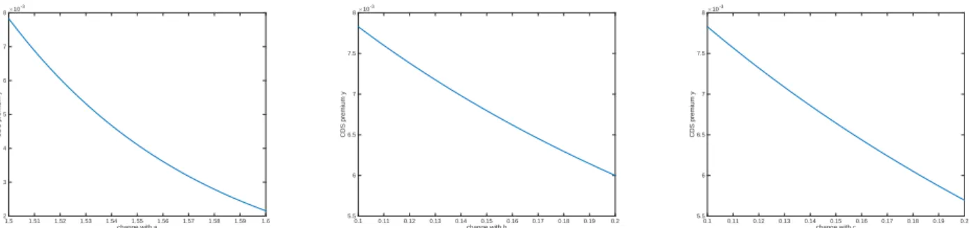
Hereτ1has the same meaning as before,τ2denotes the time of the second default in the reference portfolio. Then we can apply the methods introduced in the previous sections to calculate the fixed premium ratey. The base setting of parameters are as follows. For the contagion factors, we let a= 1, b= 0.1, c = 0.1. The expiryT is 5 years, and the initial time is 0. We change the coefficients a, band cin the expressions of default intensities separately, and each time we keep the remaining coefficients unchanged to investigate the change in the CDS premium rate y.
From the above three figures, we find that the value of CDS premium rate y decreases as the coefficients a, b, and cincrease.
change with a 1.5 1.51 1.52 1.53 1.54 1.55 1.56 1.57 1.58 1.59 1.6 CDS premium y ×10-3 2 3 4 5 6 7 8
(a) premiumychange with respect toa
change with b 0.1 0.11 0.12 0.13 0.14 0.15 0.16 0.17 0.18 0.19 0.2 CDS premium y ×10-3 5.5 6 6.5 7 7.5 8
(b) premiumychange with respect tob
change with c 0.1 0.11 0.12 0.13 0.14 0.15 0.16 0.17 0.18 0.19 0.2 CDS premium y ×10-3 5.5 6 6.5 7 7.5 8
(c) premiumychange with respect toc
Figure 1: Change of premiumy with coefficients
6.2 Numerical Example 2
We then consider a kth-to-default basket CDS contact. Assume that our portfolio contains K = 10 homogeneous entities, ifkentities out of this portfolio default prior to the expiry time, then $1 will be paid. For simplicity, this payment only occurs at the expiry time, but the payment of premium occurs at the initial time. Similar to the previous experiment, the entity i’s default intensity is given by
λi(t) =a+b·X(t) +c· X j6=i 1{τj≤t} , i, j= 1,2,· · ·, K. The value of this kth-to-default basket CDS at time tcan be written as
Vk(t) = exp{−r(T−t)}P(τk≤T | Ft)
where τk denotes the kth-to-default time. For the state of chain X, x0 and x1 represent the
“good” and “bad” economic state, respectively. While States y0 and y1 of chain Y represent
the delayed information of “bad” economic state and “good” economic state, respectively. Here we also assume that the total number of entities in the portfolio is K = 10. The calculation of P(τk≤T | F
s) can be obtained from 1−P(τjk > T | Fs) where
P(τjk > t| Fs) = k−1 X i=m P(τji ≤t < τji+1 | F s).
The calculation of the probability P(τji ≤ t < τji+1 | F
s) is similar to the calculation of
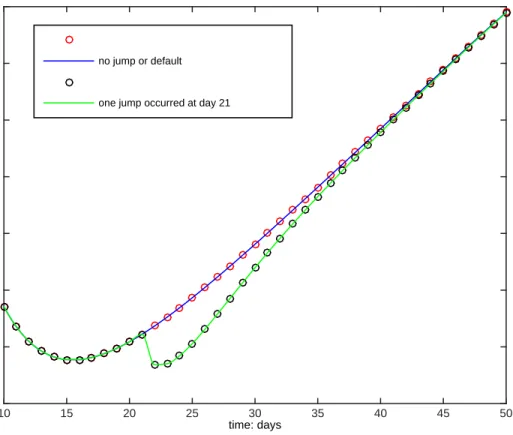
P(τ1 ≤ t < τ2) in Experiment 1. Without loss of generality, for simplicity, we consider the 1st-to-default basket CDS as k = 1. We further assume that the initial time is 0, and that we are at time t = 10 days now, and that the expiry time is T = 100 days. In the following
time: days
10 15 20 25 30 35 40 45 50
value of basket CDS along the time
0.76 0.7605 0.761 0.7615 0.762 0.7625 0.763 0.7635 no jump or default
one jump occurred at day 21
Figure 2: Change of CDS’s value from day to day with the 1st default intensities experiments, we consider two scenarios. In Scenario 1, there is no jump in chainY and default observed by expiry time. In Scenario 2, there is one jump in chain Y between day 21 and day 22 but no default observed by expiration. According to the assumptions presented in Section 2, we know that the initial state of chain X isx0= 0 and the initial state of chain Y isy0= 0. In addition, let the coefficients in default intensities be a= 0.001, b = 0.001, and c= 0.001. Then one can see the change of basket CDS values from day to day, and here we only provide the values from dayt= 10 to dayt= 50 as an example.
From the figure we can see that as time goes by, the general tendency of basket CDS’s value is increasing. When there is one jump in chainY from state y0 to statey1, the value will drop
suddenly. It is because at the beginning, the information of chain Y reflected a “bad” economic condition, when it changed to state y1 which representing a “good” economic state, intuitively,
the probability of defaults will drop suddenly, and the value of basket CDS will therefore drop suddenly as well.
time: days
10 15 20 25 30 35 40 45 50
value of basket CDS along the time
0.3725 0.373 0.3735 0.374 0.3745 0.375 0.3755 0.376 0.3765 0.377 0.3775 no jump or default one jump occurred at day 21
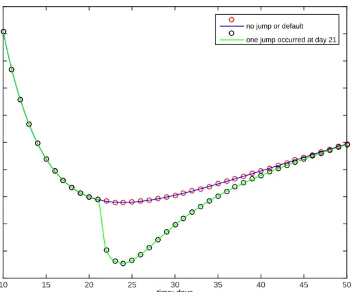
Figure 3: Change of CDS’s value from day to day with the 2nd default intensities default intensities. Therefore, we further consider another form of default intensities which decay exponentially with time. The expression is as follows:
λi(t) = a+c·X j6=i 1{τj≤t} e−t+b·X(t), i, j= 1,2, . . . , K.
Same as before, all parameters in this default intensity keep the same as the previous case, then we can also calculate the value of basket CDS and observe it from day to day.
From the figure, we notice that the overall value based on this form of default intensity is smaller than the previous one. The phenomenon can be explained as follows. As the default intensity exponentially decreased with time, the default probability will become smaller accord-ingly and therefore the value of basket CDS. For the same reason and similar explanations like before, the value will also jump down suddenly when one jump in observable chainY from state y0 toy1 occurred.
7
Concluding Remarks
In this paper we present a reduced-form intensity-based credit risk model with a hidden Markov process modeling the evolution of economic condition over time. We also discuss a method to extract the underlying hidden state process from observable processes: the default processes and the stochastic process which reflects the delayed and noisy information about the hidden state process. The method may have a wide range of applications. Based on this, we develop a closed-form expression to obtain the joint default distribution with the hidden state process. After deriving this general formula, for the homogeneous contagion portfolio, we also give analytical formulas for the distribution of ordered default times. Beside, we extend the total hazard construction method to get the joint distribution of default times for hidden markov models. We remark that the methods discussed may be applicable to various forms of default intensities. Algorithms for practical implementation of the methods are presented and their uses for pricing credit derivatives are illustrated. In the numerical experiments, we consider valuations for the CDSs premium rates of the regular and basket type with different expressions of default intensities which cover an exponential decay and a stochastic intensity process. We also study the sensitivities of premium rates with respect to changes in the underlying parameters in the regular CDS as an example.
Acknowledgements
This research work was supported by Research Grants Council of Hong Kong under Grant Number 17301214 and HKU CERG Grants and HKU strategic Research Theme in Information and Computing.
References
[1] F. Black and M. Scholes, The pricing of options and corporate liabilities, Journal of Political Economy, 81(3), 637–654, 1973
[2] D. Brigo, A. Pallavicini & R. Torresetti, Calibration of CDO tranches with the dy-namical generalized-Poisson loss model, Working Paper, Banca IMI, 2006, available at http://papers.ssrn.com/sol3/papers.cfm?abstract id=900549.
[3] R. Cont and A. Minca,Recovering portfolio default intensities implied by CDO quotes, Math-ematical Finance. doi: 10.1111/j.1467-9965.2011.00491.x, 2011
[4] M. Davis and V. Lo, Modeling default correlation in bond portfolios, in C. Alexander (Ed.), Mastering Risk Volume 2: Applications, Prentice Hall, 141-151, 2001.
[5] R. J. Elliott, M. Jeanblanc and M. Yor, (2000), On Models of Default Risk, Mathematical Finance, 10(2), 179195.
[6] R.J. Elliott and T.K. Siu, (2013),An HMM Intensity-Based Credit Risk Model and Filtering, State-Space Models and Applications in Economics and Finance, Statistics and Econometrics in Finance, Volume 1, (edited by Yong Zeng and Shu Wu), Springer-Verlag, pp. 169-184. [7] R.J. Elliott, T.K. Siu and E.S. Fung, (2014), A Double HMM Approach to Altman Z-scores
and Credit Ratings, Expert Systems With Applications, 41(4-2), pp. 1553-1560.
[8] Frey, R., and W. Runggaldier, (2010), Pricing credit derivatives under incomplete informa-tion: a nonlinear-filtering approach, Finance and Stochastics, 14 (4) pp. 495-526.
[9] Frey, R., and W. Runggaldier, (2011), Nonlinear Filtering in Models for Interest Rate and Credit Risk, Chapter 32 in Handbook of Nonlinear Filtering, D. Crisan, B. Rozovski, eds., Oxford University Press.
[10] Frey, R., and T. Schmidt, (2011) Filtering and Incomplete Information in Credit Risk, Chapter 7 in Recent Advancements in the Theory and Practice of Credit Derivatives, Dami-ano Brigo, Tom Bielecki and Frederic Patras, ed., Wiley, New Jersey.
[11] Giesecke, K. (2008),Portfolio Credit Risk: Top-Down vs. Bottom-Up Approaches, in: Fron-tiers in Quantitative Finance: Credit Risk and Volatility Modeling, R. Cont (Ed.), Wiley. [12] K. Giesecke and L. Goldberg, Sequential defaults and incomplete information, Journal of
Risk, 7(1), 1–26, 2004.
[13] K. Giesecke, L. Goldberg and X. Ding,A top down approach to multi-name credit, Opera-tions Research, 59(2), 283–300, 2011.
[14] J. Gu, W. Ching, T. Siu and H. Zheng, On pricing basket credit default swaps, Quantitative Finance, 13(12), 1845–1854, 2013.
[15] J. Gu, W. Ching and H. Zheng, A hidden Markov reduced-form risk model, Computational Intelligence for Financial Engineering & Economics, 2014 IEEE Conference, 190–196, 2014. [16] D. Duffie and N. Garleanu, Risk and valuation of collateralized debt obligations, Financial
Analysts Journal, 57(1), 41–59, 2001.
[17] D. Duffie, L. Saita and K. Wang, Multi-period corporate default prediction with stochastic covariates, Journal of Financial Economics, 83(3), 635–665, 2006.
[18] R. Jarrow and S. Turnbull,Pricing derivatives on financial securities subject to credit risk, Journal of Finance, 50, 53–86, 1995.
[19] R. Jarrow and F. Yu,Counterparty risk and the pricing of defaultable securities, Journal of Finance, 56(5), 555–576, 2001.
[20] D. Lando, On Cox processes and credit risky securities, Review of Derivatives Research, 2, 99–120, 1998.
[21] F. Longstaff and A. Rajan,An empirical analysis of collateralized debt obligations, Journal of Finance, 63(2), 529–563, 2008.
[22] R. Merton, On the pricing of corporate debt: the risk structure of interest rates, Journal of Finance, 29(2), 449–470, 1974.
[23] D. Madan and H. Unal,Pricing the risks of default, Review of Derivatives Research, 2(2-3), 121–160, 1998.
[24] I. Norros, A compensator representation of multivariate life length distributions, with ap-plications, Scand. J. Stat., 13, 99–112, 1986.
[25] M. Shaked and G. Shanthikumar, The multivariate hazard construction, Stoch. Proc. Appl, 24, 241–258, 1987.
[26] P. Sch¨onbucher and D. Schubert,Copula-dependent default risk in intensity models, Work-ing paper, Universit at Bonn, 2001.
[27] F. Yu,Correlated defaults in intensity-based models, Mathematical Finance, 17(2), 155–173, 2007.
[28] H. Zheng and L. Jiang, Basket CDS pricing with interacting intensities, Finance and stochastics, 13, 445–469, 2009.