Comparison of procedures for fitting the autoregressive order of a vector error correction model

(1)

order of a vector error correction model

Hamdi Ra¨ıssi

To cite this version:

Hamdi Ra¨ıssi. Comparison of procedures for fitting the autoregressive order of a vector error

correction model. Journal of Statistical Computation and Simulation, Taylor & Francis, 2012,

82 (10), pp.1517-1529.

<10.1080/00949655.2011.583652>.

<hal-00745885>

HAL Id: hal-00745885

https://hal.archives-ouvertes.fr/hal-00745885

Submitted on 26 Oct 2012

HAL

is a multi-disciplinary open access

archive for the deposit and dissemination of

sci-entific research documents, whether they are

pub-lished or not.

The documents may come from

teaching and research institutions in France or

abroad, or from public or private research centers.

L’archive ouverte pluridisciplinaire

HAL

, est

destin´

ee au d´

epˆ

ot et `

a la diffusion de documents

scientifiques de niveau recherche, publi´

es ou non,

´

emanant des ´

etablissements d’enseignement et de

recherche fran¸

cais ou ´

etrangers, des laboratoires

publics ou priv´

es.

(2)

AUTOREGRESSIVE ORDER OF A VECTOR ERROR

CORRECTION MODEL

Hamdi Raïssi

EQUIPPE-GREMARS, Université Lille 3 and

IRMAR-INSA

Abstract

This paper investigates the lag length selection problem of a Vector Error Correction Model (VECM) by using a convergent information criterion and tools based on the Box-Pierce methodology recently proposed in the literature. The performances of these approaches for selecting of the optimal lag length are compared via Monte Carlo experiments. The effects of misspecified deterministic trend or cointegrating rank on the lag length selection is studied. Noting that processes often exhibit nonlinearities, the cases of iid and conditionally heteroscedastic errors will be considered. Strategies which can avoid misleading situations are proposed.

Keywords: Vector error correction model; Model selection; Cointegration; Information criteria; Autocorrelation tests.

1. Introduction

The Vector Error Correction Models (VECM) are often used in the statistical analysis of nonstationary variables since they allow to describe several features. In particular the cointegration analysis of equilibrium relationships between variables is much considered in theoretical research. The dominant test for determining the number of equilibrium relationships, the cointegrating rank, is the Likelihood Ratio (LR) test developed by Johansen (1988,1991). Noting that this test depend on the specification of the deterministic part of the VECM, Johansen (1994) proposed LR tests based on his likelihood procedure for testing restrictions on the deterministic parameters. However it is well known that the likelihood inference proposed by Johansen for the analysis of the long run relationships and the deterministic terms strongly depend on the choice of the lag length. Indeed if the short run dynamics are over specified this can entail a loss of efficiency in our multivariate framework since a large number of parameters are introduced in this case. Some authors found that the LR test for the cointegrating may suffer from a substantial loss of power in such a case (see e.g. Boswijk and Franses (1992)). If the short run dynamics are under specified the residuals become autocorrelated and the asymptotic theory underlying the Johansen’s procedure breaks down (Johansen (1995), Theorem B.13 p 251). Hence the LR test for the cointegrating ∗_{Postal address: 20, avenue des buttes de Coësmes, CS 70839, F-35708 Rennes Cedex 7, France.}

mail: [email protected].

(3)

rank is not valid even asymptotically in this case. One can expect the similar effects on the LR tests for deterministic parameter restrictions when the autoregressive order is misspecified. Therefore it clearly appears that the choice of the lag length of a VECM is crucial.

When a cointegration analysis is conducted the autoregressive order is usually chosen by considering an information criterion. For instance Cavaliere, Rahbek and Taylor (2010) studied long run relationships between interest rates and used the Bayesian Information Criterion (BIC) to fit an autoregressive order to the data. Several papers have been devoted to the study of the performances of information criteria to find the optimal lag length of a VECM. Reference can be made to Ho and Sorensen (1996), Gonzalo and Pitarakis (1998) or Hacker and Hatemi (2008). These simulation investigations highlight the difficulty of choosing the autoregressive order of a VECM although the trend parameters are not taken into account in these studies. Numerous information criteria are available for the choice of the autoregressive order of VECM, as for instance the asymptotically efficient Akaike Information Criterion (AIC) or the consistent BIC. A consistent information criterion is such that the selected lag length converge to the true autoregressive order while efficiency relies on the optimal prediction error. Since in our case the main objective is to find the optimal lag length for the VECM, we restrict our attention to the commonly used BIC. Note that considering other consistent information criteria would lead to similar general conclusions.

On the other hand tests based on the autocorrelations of the residuals for checking the adequacy of the lag length in the framework of cointegrated variables have been recently proposed in the literature by Duchesne (2005), Brüggemann, Lütkepohl and Saikkonen (2006) and Raïssi (2010). Some of these tests are implemented in the software JMulTi. In this paper we compare the lag length selection properties of an consistent information criterion and of the Box-Pierce methodology with possibly mis-specified cointegrating rank or the deterministic terms. We focus on the portmanteau tests since the Box-Pierce methodology is routinely used for checking the adequacy of fitted models to time series. Using the properties of each of the methods for specifying the short run dynamics of a VECM, strategies which can reduce misleading choices for the lag length are presented. These strategies are proposed taking into account of possibly misspecified long run relations or deterministic terms, and also the possible presence of nonlinearities.

The remainder of the paper is organized as follows. Section 2 outlines the framework of our study and introduces the deterministic parameters restrictions. The estimation procedure for the VECM is described in Section 3. The tools used for model selection in the Monte Carlo experiments are also presented. In Section 4 the framework of our simulation experiments is given and the results are discussed. Strategies exploiting the properties of the Box-Pierce methodology and of information criteria lag length selection procedures are presented.

The following general notation is used throughout the paper. Considering ad×r

dimensional matrixA, we define the orthogonal complementA⊥, which is a full column rankd×(d−r)matrix such thatA′

A⊥= 0. For a given random variablea_twe define

katkq = (Ekatkq) 1/q

, where k.k denotes the Euclidean norm. The trace of a square matrix is denoted by Tr and the determinant by|.|.

(4)

2. Characterization of the model Let us consider the following VECM

∆xt=µ0+µ1t+αβ ′ xt−1+ p0−1 X i=1 Γi∆xt−i+ǫt, (2.1) where the process(xt)isd-dimensional and∆xt:=xt−xt−1. The parametersαandβ are of full column rank and of dimensiond×r0. TheΓi’s ared×dshort run parameters, and whenp0= 1the sum in (2.1) vanishes. The error process(ǫt)is commonly assumed iid Gaussian with positive definite covariance matrix Σǫ and such that Eǫt = 0. However the standard assumption of iid Gaussian errors cannot take into account of nonlinear dynamics which often arise in practice. This framework is then considered to be not realistic in many situations. For instance Trenkler (2003), Koutmos and Booth (1995) or Hiemstra and Jones (1994) studied financial variables and found a strong evidence of nonlinear dependence in the data. Numerous models in the literature produce processes with conditional heteroscedasticity as for instance hidden Markov models (see e.g. Amendola and Francq (2009)) or MGARCH models (see e.g. Bauwens, Laurent and Rombouts (2006)). Taking into account the dependence of the errors is important for testing the adequacy of linear models as pointed out by Francq, Roy and Zakoïan (2005) or Francq and Raïssi (2007). In addition the study of VECM in nonstandard situations has attracted much attention in the recent years. Therefore we also consider in our simulations the case of dependent but uncorrelated errors which are such that the results of the Granger representation theorem hold (see equation (2.3) below) as in Rahbek, Hansen and Dennis (2002), Raïssi (2009) or Hacker and Hatemi (2008).

The following restrictions on the deterministic parameters are considered

Rl: µ1=ατl ˜ Rl: µ1= 0 (2.2) Rs: µ0=ατsandµ1= 0 ˜ Rs: µ0=µ1= 0.

Note that we do not have necessarily τl 6= 0 for Rl and τs 6= 0for Rs or µ0 6= 0 for Rl, R˜l and Rs, so that we have the relation R˜s ⊂ Rs ⊂ R˜l ⊂Rl. Nested LR tests for the restrictionsR˜l, Rs and R˜s are proposed in Johansen (1995). Now we discuss the consequences of the restrictions in (2.2) on the behaviour of (xt). Suppose that

α′

⊥Γβ⊥has full rank, whereΓ =I_d−Pp0 −1

i=1 Γi. We also assume that the autoregressive polynomial A(z) = (1−z)Id−αβ′z−Pp0

−1

i=1 Γi(1−z)z

i _{is such that} _det_A₍_z_{) = 0} implies that | z |>1 or z = 1. Under these assumptions, it follows from Granger’s representation theorem (Johansen (1995), p 49) that

xt = C t X i=1 (ǫi+µ0+µ1t) +D(L)(ǫt+µ0+µ1t) +A = C t X i=1 ǫi+ρ1t+ρ0+Yt+A, (2.3)

(5)

where C=β⊥(α′_⊥Γβ⊥)−1α′_⊥ andL is the usual lag operator. The vectorA depends on initial values and verifiesβ′

A= 0. The process(Yt)is linear and such that

yt= ∞

X

i=0 φiǫt−i,

where the power seriesD(z) =P∞

i=0φiz

i_{is convergent for}_|_z_|≤_{1 +}_κ_{for some}_{κ >}₀_. The vectorsρ1,ρ0are functions of the parameters in (2.1). If we suppose thatRlhold, we may haveρ16= 0andρ06= 0and in this case(β

′

xt)can be composed of a stationary process plus a linear trend. We say in this case that (β′

xt)is trend stationary. If R˜l hold, again we may have ρ1 6= 0 and ρ0 6= 0, but (β

′

xt) is stationary. If Rs hold we obtain ρ1 = 0 but we still may have ρ0 6= 0, and in this case it is also allowed to haveE(β′

xt)6= 0. Finally the restrictionR˜s does not allow for any deterministic component for(β′

xt)and (xt). The number of independent linear combinationsβ′xt which are such that the random walk behaviour is vanished is the cointegrating rank. In particular when r0 = 0 there is no cointegration between the variables and model (2.1) is a vector autoregressive model for the process (∆xt). From (2.3) the process

(∆xt) is stationary for all the restrictions, so that (xt) is I(1). Note that we do not study the unrestricted case which produce nonstationary processes with quadratic trend since it is rarely faced in applied works. Then we see that the deterministic term and the cointegrating rank are important for the data analysis and forecasting purposes. However we will see in the next section that the specification ofµ0, µ1and r0strongly depend on the choice of the autoregressive order.

Various tests for the cointegrating rank are available in the literature (see Hubrich, Lütkepohl and Saikkonen (2001) for a review of such tests). The most commonly test for the cointegration rank is the LR test introduced by Johansen (1988,1991), which is shown to be asymptotically valid under quite general assumptions (see Rahbeket al

(2002) or Raïssi (2009)). Using the same arguments of Raïssi (2009) and following the proofs of corollary 11.2 and theorem 11.3 of Johansen (1995) it can be shown that the LR tests for the deterministic term are also asymptotically valid when the errors are dependent but uncorrelated.

3. Determining the autoregressive order

We first briefly describe the estimation procedure of the model (2.1). The reader is referred to Johansen (1995) for more details on the maximum likelihood estimation of VECM. If the errors are not assumed Gaussian, the quasi maximum likelihood is used. Let us assume that the observationsx1, . . . , xnare available. Note thatαandβ are not identified in (2.1), and in case ofRland Rsthe parametersτl andτsare also not identified. In the sequel we suppose that these parameters are normalized in some appropriate way. Let us rewrite (2.1) as follow

∆xt=θξt−1+ǫt, (3.1) where ξt−1 = ((B ′ zt−1) ′ ,∆X′ t−1, . . . ,∆X ′ t−_p0+1) ′ . We set B = (β′ , τl)′ and zt−1 = (x′ t−1, t) ′

if we suppose that Rl hold but not R˜l in (3.1). If R˜l is hold but not Rs we set B = β and zt−1 = xt−1. We consider B = (β

′ , τs)′ and zt−1 = (x ′ t−1,1) ′ if

(6)

parameters are assumed to be equal to zero. The parameters inB can be estimated using Reduced Rank (RR) regression. The super-consistency of the parameters inB

can be obtained under quite general assumptions on the error terms (see e.g. Rahbeket al (2002) or Raïssi (2009)). It is important to note that in the RR estimation method the process(ξt)is used so that the resulting estimators strongly depend on the fitted autoregressive order p > 0 which can be such that p 6= p0. As a consequence the computation of the LR tests statistics for the cointegrating rank and the deterministic terms depend onp. Therefore the choice of the autoregressive order is crucial for the cointegration analysis and the specification of the deterministic part of the model. Let us set θ = [α,Γ1, . . . ,Γp0−1, µ0] if Rl hold but not Rs and θ = [α,Γ1, . . . ,Γp0−1] if Rs hold. Once the parameter B is replaced by its estimator in (3.1) we can compute a least squares estimator for θ. However it is clear that the estimator of the short run parameters we obtain depend on the specification of cointegrating rank and of the deterministic parameters. If we suppose that the VECM is well specified, it can be shown that these estimators are asymptotically normally distributed (see Brüggemann, Lütkepohl and Saikkonen (2006) in the iid Gaussian case and Raïssi (2010) when the errors are dependent but uncorrelated).

Now we introduce the tests used in the Box-Pierce methodology. Let us denote by

ˆ

ǫtthe residuals obtained from the estimation stage. We define the residual autocovari-ances ˆ Γǫ(h) :=n−1 n X t=h+1 ˆ ǫtǫˆ ′ t−_h.

The commonly used portmanteau statistic based on the firstmautocovariances is given by Q=n m X h=1 TrΓˆǫ(h) ′_ˆ Γǫ(0) −1_ˆ Γǫ(h)ˆΓǫ(0) −1 . (3.2)

This statistic corresponds to the generalization of the Box and Pierce (1970) portman-teau statistic in the multivariate case proposed by Chitturi (1974). One can alterna-tively use the Ljung and Box (1978) portmanteau statistic proposed in the multivariate framework by Hosking (1980) for potential improvements when the errors are Gaussian. Nevertheless the use of the Ljung-Box statistic lead to the same general conclusion for our study, so that we focus on the Box-Pierce (BP hereafter) portmanteau test in the sequel. The tested hypotheses for checking the adequacy of the autoregressive order are given by

H0: E(ǫtǫt−i) = 0 vs H1: ∃isuch thatE(ǫtǫt−i)6= 0,

i∈ {. . . ,−1,0,1, . . .}are commonly considered for the portmanteau tests, although the test statistics are only based on them first residual autocorrelations. Assuming that the error process is iid Gaussian and such thatkǫtk4<∞, Brüggemann, Lütkepohl and Saikkonen (2006) showed that the asymptotic distribution of the statistic in (3.2) can be approximated by aχ2

(d2

(m−p0+ 1)−dr0)distribution whenm→ ∞asn→ ∞. Using this result they proposed a portmanteau test in the case of cointegrated variables.

(7)

This test will be denoted asBPS in the sequel. If we suppose that the errors are only uncorrelated andkǫtk4+ν <∞for someν >0and under other technical assumptions, it is shown in the framework ofR˜sin Raïssi (2010), that the asymptotic distribution of the test statistic Q is a weighted sum of chi-squares. Starting from this result a portmanteau test which is robust to the possible presence of nonlinearities in the error terms is proposed. The extension to the other restrictions considered in this paper is straightforward and is described in an extended version of Raïssi (2010) available under request. This test will be denoted asBPW. In practice the RR estimators are derived for given 0 ≤ r < d which can be such that r 6= r0. It is clear from the estimation stage that the statistic Q depend on the specified deterministic term and the fitted cointegrating rank. The effects of such possible misspecifications will be studied in the next section.

To determine the number of short run dynamics to include in the model information criteria of the form

IC = log|Γˆǫ(0)|+(p+ 1)cn/n.

are often used for a given specification of the deterministic parameters and cointegrat-ing rankr. Paulsen (1984) showed that the information criterion provide a consistent estimator of p0 if and only if cn is such that cn → ∞ and cn/n → 0. We have

cn =d2lognfor the BIC andcn= 2d2for the AIC, so that the BIC gives a consistent estimator of the lag length on the contrary to the AIC. Then we focus on the BIC in the sequel, noting that any other convergent information criterion will lead to the same general result. The BIC is computed for a set of possible values ofpand the lag length which minimizes the BIC is selected. In general the residual empirical variance

ˆ

Γǫ(0)is often used for the computation of information criteria. Then similarly to the portmanteau test statistics, we see that well specifying the cointegrating rank and/or the deterministic term is important. We also note from the BIC expressions that this approach for choosing pis not intended to detect a serial correlation of the residuals or to control any error of first kind. However we can remark that the existence of the fourth moments is not needed to compute these information criteria. In the next section we compare the two approaches for the choice of p.

4. Monte Carlo experiments

The performances of the BIC and of the tests based on the residual autocorrela-tions for selecting the autoregressive order is studied. Using these results we propose strategies which combine the use of the BP methodology and information criteria for selecting the lag length, taking into account for possibly misspecified deterministic terms or fitted cointegrating rank. In a first time the framework of the experiments is described. In each of the experiments we simulatedN = 1000independent trajectories of lengths n= 100andn= 1000using a Data Generating Process (DGP) inspired by the canonical form of Toda (1994)

xt= ψIr0 0 0 Id−r0 xt−1+ Γ01∆xt−1+µ0+µ1t+ǫt,

(8)

where ψ is a scalar and d = 4. The parameters are taken ψ = 0.5, Γ01 = −0.3I4 and the cointegrating rank is r0 = 2. We set µ1 = (−0.05,−0.05,0,0)

′

and µ0 =

(0.1,0.1,0.1,0.1)′

ifRlis hold but notR˜l. The results for the case of simulated processes such that Rs is hold but not R˜s are not displayed since they are similar to the case

µ0 =µ1 = 0. In the sake of conciseness the results for the restriction R˜l is hold but notRs are not displayed since they lead to similar conclusions to the cases presented here. This kind of DGP is used in numerous studies (e.g. Hubrich et al (2001) or Demetrescu et al (2009)). In addition the results concerning the information criteria are corroborated by previous studies. In the experiments the cointegrating rank and the deterministic terms are not necessarily well fitted, so that the consequences of such situations is analyzed. Since the number of parameters is high, a relatively large samples are taken in our experiments. Two cases are considered for the error process in the sequel. In case of iid innovations we takeǫt∼ N(0, Id). To illustrate the case where the errors are dependent, we use the following ARCH model with constant correlation of Jeantheau (1998)    ǫ1t .. . ǫdt   =    σ1t 0 0 0 . .. 0 0 0 σdt       η1t .. . ηdt    (4.1) where    σ2 1t .. . σ2 dt   =    0.1 .. . 0.1   +     0.2 0 0 0.1 0.1 0.2 0 0.1 0.1 0 0.2 0.1 0.1 0 0 0.2        ǫ2 1t−1 .. . ǫ2 dt−1   ,

and the processηt= (η1t, . . . , ηdt) ′

is iid, such thatηt∼ N(0, Id).

The autoregressive order selection strategy correspond to the case where the prac-titioner have no prior knowledge on p0. More precisely for the portmanteau tests p= 1,2, . . . are successively tested until the null hypothesis is not rejected. However we assume that when the autoregressive order adequacy is rejected for allp≤5, the model specification is suspected to be not reliable and one stop the procedure. Indeed whenptakes large values the number of parameters become high beside the available observations. In such case the analysis of the linear dynamics is not reliable. In our experiments we used the asymptotic nominal level 5% for the different portmanteau tests considered in this paper. In the sequel note that if the portmanteau tests perform well, the selectedp=p0is often around 95% since this selection procedure is based on the control of the error of first kind. Note that theBPW test is available for fixedm, while for theBPS it is assumed that m → ∞as T → ∞. Thereforem= 5 is taken for theBPW test forT = 100 andT = 1000, while we takem= 5 whenT = 100and

m = 15 whenT = 1000 for the BPS test. The autoregressive order which minimize the BIC in the set{1, . . . ,5}is selected. The results are given in Tables 1-12.

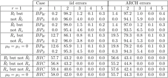
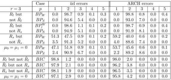
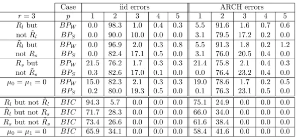
We first analyze the results for small samples (T = 100) given in Tables 1-6. It appears that the performances of the BPW test is rather disappointing. This can be explained by the fact that about 40 parameters are estimated when p = 2and thus the number of observations is relatively small for the elaboratedBPW test. In such situation the more simple BPS test provide satisfactory results. It seems that the results for the portmanteau tests are not much affected when the deterministic terms

(9)

or the cointegrating are misspecified in small samples. We only remark that when a deterministic trend present in the data is not taken into account by the practitioner (Tables 4-6), theBPS test tends to select a too large lag length. From Tables 1-6 we see that the BIC selects a too smallp. Whenr < r0is taken the BIC is likely to choose a larger autoregressive order. Therefore it seems that the use of the parsimonious BIC when the sample is small can be misleading for the analysis of VECM.

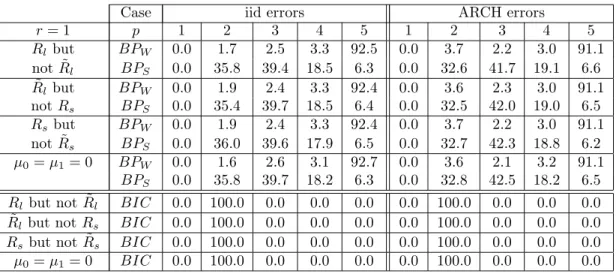
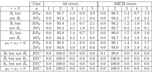
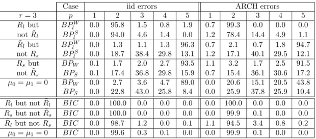
Now we consider the results for large samples (T = 1000). It is found from Tables 7-12 that theBP tests perform well when the long run relations and the deterministic terms are well specified. However we note that when r < r0 is taken, the BP tests tend to select too large autoregressive orders. If r < r0 the estimators of the short run parameters are biased and the residual autocorrelations may appear too large as the sample increase even if p = p0. When r > r0 is taken we note that the BP tests are not much affected. A possible explanation is that in this case the effect of non stationary components introduced in the model are limited by the fact that the corresponding adjustment parameters are close to zero. It is important to note that overspecified deterministic terms seems not entail a significant loss of efficiency in selecting the autoregressive order using theBP methodology. However from Tables 10-12 we see that the BP tests are clearly likely to select a too large autoregressive order when a deterministic trend is present in the observed process and is not taken into account in the model. Similarly we also found from Tables 10-12 that when deterministic trends are spuriously assumed to not enter the cointegrating relations the BP tests select too largep. When the BP tests are used and in case of doubt, it seems preferable to consider the restriction Rl only for fitting the autoregressive order. In such situations the unnecessary parameters introduced in the model are few. Actually we noted no major loss of efficiency and considering such restriction allow to avoid misspecified autoregressive order. Of course as pointed out by several studies (e.g. Johansen (1994)) it is important to remove any misspecification of the deterministic term when determining the cointegrating rank. Finally it emerges that in general theBPW test is not affected by the presence of dependent errors. In some cases theBPS test tends to select too largepwhen the errors follow an ARCH model. This can be explained by the fact that theBPS is not intended to take into account such situations. In accordance with the theoretical, we found that the BIC choose successfully the optimal lag length when the sample is large in both standard and dependent cases. It also appears that the selected autoregressive orders do not depend much on the specification of the deterministic terms or on the fitted cointegrating rank. Nevertheless it is important to note that the use of information criteria for fitting the lag length can be quite misleading even when the sample is large. For instance we give the autoregressive order selected by the AIC criterion for the case given in Table 10. Despite the VECM is well specified, the AIC select a too large p. Results not reported here show that the AIC almost always choose a lag length p= 5 in many of the situations presented here. This is not surprising since for the AIC the more complicated models are not so penalized. Thereby this confirms that the BIC perform better than the AIC for the lag selection (see e.g. Cheung and Lai (1993) or Ho and Sorensen (1996)).

(10)

5. Conclusion

In this paper we studied the problem of the fit of the autoregressive order by com-paring tools based on the Box-Pierce methodology recently proposed in the literature and information criteria commonly used in practice. Fitting an adequate autoregres-sive order is important for the analysis of VECM, but this task is carried out using information criteria only in general. It emerges from our study that underspecified deterministic trend or cointegrating rank can be quite misleading when using the Box-Pierce methodology for the choice of the autoregressive orderp. We also found that the selection ofpusing information criteria does not depend much on the specification of the other parts of the model. However the use of these information criteria can be quite misleading in some cases. In general we recommend to use the information criteria together with the portmanteau tests when choosing the lag length of a VECM. When the selected autoregressive orders are close and small, then one should take thepproposed by the portmanteau tests. It is advisable to choose the pselected by the portmanteau tests since they are able to detect residual autocorrelations which can strongly affect the cointegration analysis. If the lag lengths selected by the two approaches presented in this paper are both large, it is important that the chosen information criterion is parsimonious to conclude on the reliability of the selected lag length. If thepretained by an information criterion is much larger than thepretained by the portmanteau tests, then one can suspect that the more complicated model is not penalized enough by the information criterion. On the other hand if thepselected using the portmanteau tests is much larger than thepselected by using an information criterion, one can suspect that the deterministic trend is underspecified or the fitted cointegrating rank is smaller the the true cointegrating rank.

References

Amendola, A. and Francq, C. (2009) Concepts and tools for nonlinear time series modelling. Handbook of Computational Econometrics, (eds: D. Belsley

andE. Kontoghiorghes, Wiley.

Bauwens, L., Laurent, S. and Rombouts, J.V.K.(2006) Multivariate GARCH models: A survey. Journal of Applied Econometrics 21, 79-109.

Boswijk, P. and Franses, P.H. (1992) Dynamic specification and cointegration.

Oxford Bulletin of Economics and Statistics 54, 369-381.

Box, G.E.P. and Pierce, D.A. (1970) Distribution of residual autocorrelations in autoregressive-integrated moving average time series models. Journal of the

American Statistical Association 65, 1509-1526.

Brüggeman, R., Lütkepohl, H. and Saikkonen, P.(2006) Residual autocorre-lation testing for error correction models. Journal of Econometrics134, 579-604.

Cavaliere, Rahbek and Taylor (2010) Testing for co-integration in vector au-toregressions with non-stationary volatility. Journal of Econometrics 158, 7-24.

Cheung, Y-W, and Lai, K.S. (1993) Finite-sample sizes of Johansen’s likelihood ratio tests for cointegration. Oxford Bulletin of Economics and Statistics 55, 313-328.

(11)

Chitturi, R. V.(1974) Distribution of residual autocorrelations in multiple autore-gressive schemes. Journal of the American Statistical Association 69, 928-934.

Demetrescu, M., Lütkepohl, H. and Saikkonen, P. (2009) Testing for the cointegrating rank of a vector autoregressive process with uncertain deterministic trend term. Econometrics Journal 12, 414-435.

Duchesne, P.(2005) Testing for serial correlation of unknown form in cointegrated time series models. Annals of the Institute of Statistical Mathematics57, 575-595.

Francq, C. and Raïssi, H.(2007) Multivariate portmanteau test for autoregressive models with uncorrelated but nonindependent errors. Journal of Time Series

Analysis 28, 454-470.

Francq, C., Roy, R. and Zakoïan, J-M. (2005) Diagnostic checking in ARMA models with uncorrelated errors. Journal of American Statistical Association

100, 532-544.

Gonzalo, J. and Pitarakis, J-Y.(1998) Specification via selection in vector error correction models. Economics Letters 60, 321-328.

Hacker, R.S. and Hatemi, A. (2008) Optimal lag-length choice in stable and unstable VAR models under situations of homoscedasticity and ARCH. Journal

of Applied Statistics 35, 601-615.

Hiemstra, C. and Jones, J.D. (1994) Testing for linear and nonlinear Granger causality in the stock price-volume relation. Journal of Finance 14, 1639-1664.

Ho, M.S. and Sørensen, B.E. (1996) Finding cointegration rank in high dimen-sional systems using the Johansen test: an illustration using data based Monte Carlo simulations. Review of Economics and Statistics 78, 726-732.

Hosking, J. R. M. (1980) The multivariate portmanteau statistic. Journal of the

American Statistical Association 75, 343-386.

Hubrich, K., Lütkepohl, H. and Saikkonen, P. (2001) A review of systems cointegration tests. Econometrics Reviews 20, 247-318.

Jeantheau, T. (1998) Strong consistency of estimators for multivariate ARCH models. Econometric Theory 14, 70-86.

Johansen, S. (1988) Statistical analysis of cointegration vectors. Journal of

Eco-nomic Dynamics and Control 12, 231-254.

Johansen, S. (1991) Estimation and hypothesis testing of cointegration vectors in gaussian vector autoregressive models. Econometrica 59, 1551-1580.

Johansen, S. (1994) The role of the constant and linear terms in cointegration analysis of non-stationary variables. Econometric Reviews 13, 205-229.

Johansen, S.(1995)Likelihood-Based Inference in Cointegrated Vector

(12)

Koutmos, G. and Booth, G.G. (1995) Asymmetric volatility transmission in international stock markets. Journal of International Money and Finance 14, 747-762.

Ljung, G.M. and Box, G.E.P. (1978) On measure of lack of fit in time series models. Biometrika 65, 297-303.

Paulsen, J. (1984) Order determination of multivariate autoregressive time series with unit roots. Journal of Time Series Analysis 5, 115-127.

Rahbek, A., Hansen, E., Dennis, J.G.(2002) ARCH innovations and their impact on cointegration rank testing. University of Copenhagen. http://www.math.ku. dk/∼rahbek/publications/ARCHCOINTJune02.pdf.

Raïssi, H. (2009) Testing the cointegrating rank with uncorrelated but dependent errors. Stochastic Analysis and Applications 27, 24-50.

Raïssi, H.(2010) Autocorrelation based tests for vector error correction models with uncorrelated but nonindependent errors. Test 19, 304-324.

Toda, H.Y.(1994) Finite sample properties of likelihood ratio tests for cointegrating ranks when linear trends are present. Reviews of Economics and Statistics 76, 66-79.

Trenkler, C.(2003) The polish exchange rate system: A unit root and cointegration analysis. Empirical Economics 28, 839-860.

(13)

Tables

Table1: Frequency (in %) of selected lag length using the portmanteau tests. The simulated processes are of lengthT = 100_{, such that}R˜s hold andr0= 2.

Case iid errors ARCH errors

r= 2 p 1 2 3 4 5 1 2 3 4 5 Rlbut BPW 0.2 98.5 1.1 0.0 0.2 1.4 97.6 0.9 0.0 0.1 notR˜l BPS 0.0 97.2 2.8 0.0 0.0 0.0 96.1 3.9 0.0 0.0 ˜ Rlbut BPW 0.2 98.6 1.0 0.1 0.1 1.4 97.7 0.6 0.0 0.3 notRs BPS 0.0 97.0 3.0 0.0 0.0 0.0 96.3 3.7 0.0 0.0 Rsbut BPW 48.1 50.9 0.8 0.1 0.1 55.2 44.1 0.6 0.0 0.1 notR˜s BPS 4.7 92.9 2.4 0.0 0.0 5.3 91.7 3.0 0.0 0.0 µ0=µ1= 0 BPW 45.8 53.2 0.8 0.1 0.1 52.8 46.4 0.7 0.0 0.1 BPS 3.7 93.6 2.7 0.0 0.0 4.0 92.6 3.4 0.0 0.0

Rl but notR˜l BIC 96.6 3.4 0.0 0.0 0.0 95.1 4.9 0.0 0.0 0.0

˜

Rl but notRs BIC 96.4 3.6 0.0 0.0 0.0 94.9 5.1 0.0 0.0 0.0

Rs but notR˜s BIC 97.0 3.0 0.0 0.0 0.0 95.3 4.7 0.0 0.0 0.0

µ0=µ1= 0 BIC 96.4 3.6 0.0 0.0 0.0 94.9 5.1 0.0 0.0 0.0

Rl but notR˜l BIC 57.7 43.2 0.0 0.0 0.0 56.6 43.4 0.0 0.0 0.0

˜

Rl but notRs BIC 56.8 43.2 0.0 0.0 0.0 55.2 44.8 0.0 0.0 0.0

Rs but notR˜s BIC 59.4 40.6 0.0 0.0 0.0 57.6 42.4 0.0 0.0 0.0

(14)

r= 3 p 1 2 3 4 5 1 2 3 4 5 Rlbut BPW 0.0 98.7 0.9 0.1 0.3 0.0 98.8 0.8 0.0 0.4 notR˜l BPS 0.0 94.6 5.4 0.0 0.0 0.0 93.0 7.0 0.0 0.0 ˜ Rlbut BPlW 0.0 98.6 1.1 0.1 0.2 0.0 98.7 0.9 0.0 0.4 notRs BPS 0.0 94.9 5.1 0.0 0.0 0.0 91.9 8.1 0.0 0.0 Rsbut BPW 51.3 47.5 0.9 0.1 0.2 59.2 40.0 0.6 0.0 0.2 notR˜s BPS 3.5 91.3 5.2 0.0 0.0 4.0 88.6 7.4 0.0 0.0 µ0=µ1= 0 BPW 47.1 51.8 0.9 0.1 0.1 53.7 45.6 0.6 0.0 0.1 BPS 2.4 90.9 6.7 0.0 0.0 2.2 89.2 8.6 0.0 0.0

Rl but notR˜l BIC 98.8 1.2 0.0 0.0 0.0 98.0 2.0 0.0 0.0 0.0

˜

Rl but notRs BIC 97.9 2.1 0.0 0.0 0.0 96.2 3.8 0.0 0.0 0.0

Rs but notR˜s BIC 98.1 1.9 0.0 0.0 0.0 96.5 3.5 0.0 0.0 0.0

µ0=µ1= 0 BIC 97.1 2.9 0.0 0.0 0.0 95.8 4.2 0.0 0.0 0.0

Table4: Frequency (in %) of selected lag length using the portmanteau tests. The simulated processes are of lengthT = 100_{, such that}Rlhold but notR˜landr0= 2.

r= 2 p 1 2 3 4 5 1 2 3 4 5 Rlbut BPlW 0.2 98.5 1.1 0.1 0.1 2.7 94.3 2.1 0.7 0.2 notR˜l BPlS 0.0 94.4 5.6 0.0 0.0 0.0 89.4 10.5 0.1 0.0 ˜ Rlbut BPlW 0.2 97.4 1.7 0.2 0.5 2.7 94.6 1.7 0.3 0.7 notRs BPlS 0.0 90.9 9.1 0.0 0.0 0.0 87.6 12.3 0.1 0.0 Rsbut BPW 21.3 76.7 1.6 0.1 0.3 26.3 71.6 1.5 0.3 0.3 notR˜s BPS 0.5 92.6 6.9 0.0 0.0 0.3 82.6 16.9 0.2 0.0 µ0=µ1= 0 BPW 16.6 81.6 1.4 0.2 0.2 21.7 76.4 1.4 0.3 0.2 BPS 0.4 91.6 7.9 0.1 0.0 0.2 83.5 16.1 0.2 0.0

Rl but notR˜l BIC 89.0 11.0 0.0 0.0 0.0 67.1 32.9 0.0 0.0 0.0

˜

Rl but notRs BIC 67.0 33.0 0.0 0.0 0.0 61.3 38.7 0.0 0.0 0.0

Rs but notR˜s BIC 71.4 28.6 0.0 0.0 0.0 52.2 47.8 0.0 0.0 0.0

(15)

Rl but notR˜l BIC 48.6 51.4 0.0 0.0 0.0 44.2 55.8 0.0 0.0 0.0

˜

Rl but notRs BIC 45.1 54.9 0.0 0.0 0.0 43.8 56.2 0.0 0.0 0.0

Rs but notR˜s BIC 55.5 44.5 0.0 0.0 0.0 57.1 42.9 0.0 0.0 0.0

µ0=µ1= 0 BIC 54.3 45.7 0.0 0.0 0.0 56.9 43.1 0.0 0.0 0.0

Rl but notR˜l BIC 94.3 5.7 0.0 0.0 0.0 75.1 24.9 0.0 0.0 0.0

˜

Rl but notRs BIC 71.7 28.3 0.0 0.0 0.0 66.0 34.0 0.0 0.0 0.0

Rs but notR˜s BIC 73.4 26.6 0.0 0.0 0.0 61.6 38.4 0.0 0.0 0.0

(16)

Table7: Frequency (in %) of selected lag length using the portmanteau tests. The simulated processes are of lengthT = 1000_{, such that}R˜shold andr0= 2.

Rl but notR˜l BIC 0.0 100.0 0.0 0.0 0.0 0.0 100.0 0.0 0.0 0.0

˜

Rl but notRs BIC 0.0 100.0 0.0 0.0 0.0 0.0 100.0 0.0 0.0 0.0

Rs but notR˜s BIC 0.0 100.0 0.0 0.0 0.0 0.0 100.0 0.0 0.0 0.0

µ0=µ1= 0 BIC 0.0 100.0 0.0 0.0 0.0 0.0 100.0 0.0 0.0 0.0

Rl but notR˜l BIC 0.0 100.0 0.0 0.0 0.0 0.0 100.0 0.0 0.0 0.0

˜

Rl but notRs BIC 0.0 100.0 0.0 0.0 0.0 0.0 100.0 0.0 0.0 0.0

Rs but notR˜s BIC 0.0 100.0 0.0 0.0 0.0 0.0 100.0 0.0 0.0 0.0

(17)

Rl but notR˜l BIC 0.0 100.0 0.0 0.0 0.0 0.1 99.9 0.0 0.0 0.0

˜

Rl but notRs BIC 0.0 100.0 0.0 0.0 0.0 0.0 100.0 0.0 0.0 0.0

Rs but notR˜s BIC 0.0 100.0 0.0 0.0 0.0 0.0 100.0 0.0 0.0 0.0

µ0=µ1= 0 BIC 0.0 100.0 0.0 0.0 0.0 0.0 100.0 0.0 0.0 0.0

r= 2 p 1 2 3 4 5 1 2 3 4 5 Rl but BPlW 0.0 96.0 1.7 0.7 1.6 0.0 100.0 0.0 0.0 0.0 notR˜l BPlS 0.0 95.0 4.0 1.0 0.0 0.0 82.9 12.2 3.9 1.0 ˜ Rl but BPlW 0.0 1.4 1.3 1.5 95.8 0.0 2.1 0.9 1.7 95.3 notRs BPlS 0.0 23.8 41.0 24.7 10.5 0.0 21.4 42.7 26.0 9.9 Rsbut BPW 0.3 1.4 1.4 1.9 95.0 0.5 2.6 1.8 2.0 93.1 notR˜s BPS 0.3 19.5 40.2 27.4 12.6 0.1 17.1 37.5 29.6 15.7 µ0=µ1= 0 BPW 0.0 2.2 3.4 5.1 89.3 0.1 18.3 14.8 20.8 46.0 BPS 0.0 27.0 43.9 21.8 7.3 0.1 29.0 38.4 23.4 9.1 Rl but AIC 0.0 0.0 0.0 0.0 100.0 0.0 0.0 0.0 0.0 100.0 notR˜l BIC 0.0 100.0 0.0 0.0 0.0 0.0 100.0 0.0 0.0 0.0 ˜ Rl but AIC 0.0 0.0 0.0 0.0 100.0 0.0 0.0 0.0 0.0 100.0 notRs BIC 0.0 99.8 0.2 0.0 0.0 0.0 100.0 0.0 0.0 0.0

Rsbut not AIC 0.1 0.0 0.0 0.0 99.9 0.7 0.1 0.1 0.7 98.4

˜

Rs BIC 0.0 98.2 1.7 0.0 0.0 0.7 93.9 4.5 0.7 0.2

µ0=µ1= 0 AIC 0.0 0.0 0.0 0.0 100.0 0.1 0.0 0.0 0.0 99.9 BIC 0.0 99.9 0.1 0.0 0.0 0.1 99.4 0.5 0.0 0.0

(18)

Rl but notR˜l BIC 0.0 100.0 0.0 0.0 0.0 0.0 100.0 0.0 0.0 0.0

˜

Rl but notRs BIC 0.0 100.0 0.0 0.0 0.0 0.0 100.0 0.0 0.0 0.0

Rs but notR˜s BIC 0.0 100.0 0.0 0.0 0.0 0.0 98.7 1.3 0.0 0.0

µ0=µ1= 0 BIC 0.0 100.0 0.0 0.0 0.0 0.0 99.8 0.2 0.0 0.0

Rl but notR˜l BIC 0.0 100.0 0.0 0.0 0.0 0.0 100.0 0.0 0.0 0.0

Rs but notR˜s BIC 0.0 100.0 0.0 0.0 0.0 0.0 99.9 0.1 0.0 0.0