Dottorato di Ricerca in
Metodologia Statistica per la Ricerca Scientifica XXI ciclo
Alma
Mater
Studiorum
-Univ
ersit`
a
di
Bologna
Multiple testing in spatial epidemiology:
a Bayesian approach
Massimo Ventrucci
Dipartimento di Scienze Statistiche “P. Fortunati” Marzo 2009
Dottorato di Ricerca in
Metodologia Statistica per la Ricerca Scientifica XXI ciclo
Alma
Mater
Studiorum
-Univ
ersit`
a
di
Bologna
Multiple testing in spatial epidemiology:
a Bayesian approach
Massimo Ventrucci
Coordinator Tutor
Professor Daniela Cocchi Professor Daniela Cocchi
Co-tutor Professor Marian Scott
Settore Disciplinare SECS-S/01
Dipartimento di Scienze Statistiche “P. Fortunati” Marzo 2009
Acknowledgments 2
Introduction 4
1 Basic concepts on Multiple Testing 9
1.1 False Discovery Rate . . . 10
1.2 Frequentist methods . . . 11
1.3 Bayesian methods . . . 12
1.3.1 Posterior probability adjustment for multiple testing . . . 14
2 Multiple testing on large datasets of Standardized Mortality Ratios 15 2.1 The rationale of the work . . . 17
2.1.1 The small areas issue . . . 18
2.1.2 The inferential approach . . . 18
2.2 Standardized Mortality or Morbidity Ratios . . . 20
2.3 The multiple testing framework . . . 23
2.3.1 Mapping significance or mapping Relative risks . . . 24
2.3.2 P-values computation in small areas . . . 26
2.3.3 The Over-dispersion issue . . . 27
2.4 Traditionalp-value based procedures for SMR multiple testing . . . 31
2.4.1 Additional remarks on multiple testing issue and over-dispersion . . . 32
3 A Bayesian Hierarchical model for False Discovery Rate estimation 37 3.1 Bayesian disease mapping . . . 37
3.1.1 Independent prior . . . 39
3.1.2 Spatially structured prior . . . 41
3.1.3 The Besag York Molli`e (BYM) model . . . 43
3.2 FDR estimation through posterior probabilities . . . 45 1
3.2.1 Our model proposal: BYM mix . . . 46
3.2.2 Full conditional distributions . . . 49
3.3 F DRd based decision rules . . . 52
4 Simulation study 55 4.1 Objectives of the simulation study . . . 56
4.1.1 Factors controlled by simulation . . . 58
4.1.2 Spatially correlated scenarios . . . 60
4.1.3 Multinomial sampling vs Poisson sampling . . . 66
4.1.4 MCMC based inference . . . 69
4.2 Evaluating model performance . . . 69
4.2.1 Measures introduced for evaluating model performance . . . 71
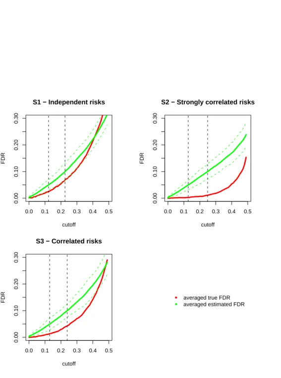
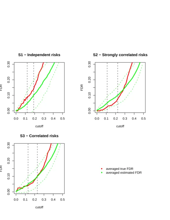
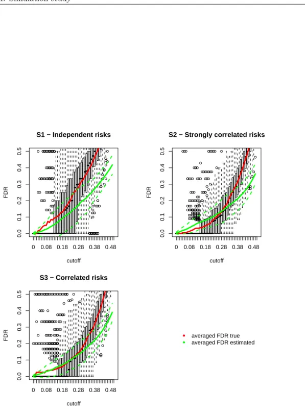
4.2.2 Summary graphs . . . 74
4.3 Results . . . 75
4.3.1 The BYM mix performance on F DR estimation . . . 75
4.3.2 TheBYM mix power in identifying at risk-areas byF DRd based selection rules 78 4.3.3 The BYM mix performance on relative risk estimation . . . 88
4.4 Conclusive remarks on the simulation study results . . . 88
4.4.1 An application to a real dataset . . . 91
Conclusions and perspectives 92
Appendix 100
A All results 101
Acknowledgments
I would like to express my sincere gratitude to my supervisor Professor Daniela Cocchi for the continuous support demonstrated during the last three years, the helpful suggestions and advices she gave me.
I am deeply indebted to my co-tutor Professor Marian Scott who helped me to approach many practical problems during my experience at the Statistics Department of the Glasgow University, providing me a constant support.
A special thanks goes also to Fedele Greco, Francesca Bruno, Carlo Trivisano, Michele Scagliarini, Rossella Miglio Clarissa Ferrari and Fabio Di Narzo who shared ideas about my work in many meetings. I cannot forget to especially thank Fedele, I very much appreciated time and energy he put into our fruitful discussions.
I had a very special moment in Glasgow and I would like to thank all professors, researchers, post-graduates and friends with whom I shared ideas and had very happy moments. Thus, thank you to Maria, Raul, Laura, Irene, Sara, Giorgio, Erik, Paolo and Jude.
A special thought goes to all friends met in the last three years in Bologna, everyone played a role in some sense and I cannot forget it. I cannot also forget my PhD colleagues, so thanks to Davide, Clarissa, Ida, Anna, Maria Serena, Elena.
A special thanks goes to Christian who can make me sure to have a good friend. Thank you to Federica for exactly the same reason.
Another special thought goes to my best friends in my village, who always wait for me to going back home, whereas I rarely do it. Also thanks, perhaps, to whom wait for me no longer.
In conclusion, I cannot forget to thank my family for the support they always provide me: Liliana, Giorgio, Stefano, Antonietta, Lino and finally Tommaso who cannot yet read these pages.
In this work we propose a new approach for preliminary epidemiological studies on Standardized
Mortality Ratios (SM R) collected in many spatial regions. A preliminary (also called descriptive)
analysis in this field aims to formulate hypotheses to be investigated via individual epidemiological studies that avoid bias introduced by aggregated analyses.
Starting from collecting disease counts yi, calculating expected disease counts ei by means of
reference population disease rates, and assuming each areaicount is distributed as a Poisson with
mean (ei·ri), anSM Ri = yeii is derived as the ML estimate of the parameterri, that is the relative
risk for the disease under examination in area i. Such estimators have high standard errors when
referred to small areas, i.e. areas where the expected count ei is low either because of the small
number of people living in the area or the rarity of the disease under study. Therefore, the presence of small areas yields maps of ML relative risk point estimates that are discontinuous; when the
expected count is very low (even lower than 1) a hugeSM Rvalue may be caused by the occurrence
of few disease cases. As a result a map ofSM Rs will tend to only highlight risk in poorly populated
areas. If we undertake a hypothesis testing inferential approach, so evaluating the null hypothesis
of absence of risk (H0i :ri = 1) against the alternative of a higher risk (H1i :ri >1) in each area
i by means of p-values computed with Poisson c.d.f., we meet the opposite problem: the test is
more likely to be significant (more powerful) in non-small areas than in small areas, hence a map
ofp-values will tend to only highlight risk in high population areas.
Disease mapping models providing maps of smoothed relative risk estimates and other tech-niques for screening disease rates on the map, that aim to detect possible high-risk areas, have been proposed in the literature according to the classical and the Bayesian paradigm. Our proposal ap-proaches this issue through a decision-oriented method: we want to evaluate many null hypotheses focusing on multiple testing control, without however leaving the “preliminary study” perspective. More precisely, we implement a multiple testing procedure that controls the False Discovery Rate
(F DR), i.e. the number of falsely rejected null hypotheses (false discoveries) divided by the number
of rejected null hypotheses (discoveries). This quantity is largely used to address multiple com-parisons problems in the field of microarray data analysis but it is not usually employed either in
testing many hypotheses on a large SM Rs dataset or in disease mapping applications, that are not concerned with testing hypotheses but only with point estimation of true relative risk values.
Controlling the F DR means providing an estimate of the proportion of false discoveries for a set
of discoveries, where a discovery is a declared high-risk area.
The presence of small areas and of positive spatial correlation between risks, that are frequently
encountered in practice, create difficulties in applyingp-value based traditional methods forF DR
control/estimation (Benjamini and Hochberg, 1995; Storey, 2003) because the necessary
distribu-tional assumptions on the p-values do not generally hold. More precisely, the p-values cannot be
assumed as independent when spatial correlation between risks is expected; furthermore they are
not identically distributed under the null hypothesis asU(0,1) when the population underlying the
map is non-homogeneous, counts are sparse, and hence over-dispersion is expected.
The Bayesian paradigm offers a way to overcome the inappropriateness ofp-value based
meth-ods. In the present work we propose a hierarchical full Bayesian model for F DR estimation in a
testing framework where many null hypotheses of absence of risk are evaluated on the observed
SM Rs. We want to focus on cases whereSM Rs are collected in small areas and risks are spatially
correlated, i.e. in cases where there is a lack of fit of the usually assumed Poisson model for indepen-dent counts. We will use concepts of Bayesian modeling for disease mapping, referring in particular
to the Besag York and Molli´e model (Besag York and Molli´e, 1991) often used in practice for its
prior assumptions flexibility w.r.t the distribution of risk parameters r = (r1, ..., rN) in the whole
map. The borrowing of strength between prior and likelihood typical of a hierarchical Bayesian
model takes advantage of evaluating the test in a given area iby means of all observations in the
map under study (y= (y1, ..., yN)) rather than just by means of the observation in the given area
(yi). This can improve the power of the test in small areas and addresses more appropriately the
spatial correlation issue that suggests that relative risks are closer in spatially contiguous regions. In practice, the proposed model aims primarily to make the practitioner able to declare a number of areas as high-risk areas (i.e. to reject a number of null hypotheses) controlling a desired level
of F DR fixed a priori. Another peculiarity is its capability to still provide posterior estimates of
relative risk values, that are the inferential target of the Besag York and Molli´e model. As regards
the primary aim, we can obtain an estimate of the False Discovery Rate through MCMC estimation
of each area specific posterior probability that the null hypothesis is true, denoted asπi =P(H0i|y).
To be precise, we will focus on controlling the expected F DR conditional on data (Broet et al.,
2004), denoted as F DR\. This quantity can be worked out given any set ofπbi’s by computing the
empirical mean over them; the key point is that eachπbiis an estimate of the type I error probability
to the areas declared at high-risk, and F DR\ as an estimate of the proportion of false discoveries which can occur in making such declarations.
The most interesting aspect of the work is the capability of the model to provide a non-arbitrary
decision rule for rejecting null hypotheses that is based on the knowledge of \F DR; we call such
rules “\F DR based decision (or selection) rules”. In a formal sense, a decision rule is defined as a
function of the πbi’s and a threshold tπ, such that if πbi ≤ tπ, then H0i (i.e. ri = 1) is rejected in
favor of the alternativeH1i (i.e. ri >1). By applying for instance an F DR\=cbased rule, where
c is the pre-fixed F DR level, the practitioner can select as many as possible areas such that the
\
F DR ≥ c. The sensitivity and specificity of such rules depend on the goodness of estimation of
the F DR. On this note, what is required in order to achieve a control is a “conservative” F DR
estimation (Storey, 2002), that is\F DR≥true F DR.
A simulation study to evaluate the model performance inF DRestimation in terms of accuracy,
sensitivity and specificity of the decision rule, and not least the performance in goodness of esti-mation of relative risks, was set up. We chose a real map from which we generated several spatial scenarios whose simulated disease counts vary according to the spatial correlation degree, the size
of the areas, the number of areas where the alternative hypothesis is true (HRareas) and the risk
level in the HR areas. For each dataset (in total 100) of each scenario (in total 54) the model
was ran using BRugs package (version 0.4 - 1) that implements OpenBUGS version 3.0.2. The
main aim of the simulation is evaluating which F DR levels are conservatively estimated (i.e. not
under-estimated) by the model in each scenarios, focusing the interest in small areas and spatially correlated risks scenarios.
An application to real data is finally presented to show the two kinds of maps that the method can produce: a map of posterior relative risk estimates and a map of highlighted high-risk areas
given a pre-chosen value of \F DR.
The plan of the work is as follows. In chapter 1 the basic concepts of F DR and multiple
testing are illustrated. Chapter 2 introduces the spatial epidemiological case study, the motivation
of the work and the multiple hypothesis setting based on SM Rs. In chapter 3 we discuss the
characteristics of the proposed model to estimate the expectF DR conditional on data. Chapter 4
Basic concepts on Multiple Testing
In evaluating a null hypothesis H0 we need a decision rule d(z(y), ty), function of a summary
statistics of dataz(y) and a thresholdtz, to decide whether or notH0 can be rejected. In
Neyman-Pearson theory, for instance, this function is ruled out such that the type I error probability
(probability of rejecting the null hypothesis when it is true) cannot be greater than a pre-chosen
levelα. Traditionally, the most typical case is when the null hypothesis is evaluated by means of
a p-value dependent on a chosen summary statistics of data z(y) and on distributional
assump-tion for z(y); a p-value is calculated as the probability of randomly occurring values at least as
unlikely as the observed z(y). Rejecting the null hypothesis when the calculated p-value is less
than the threshold tp−value = α guarantee the control of the typeI error probability in doing a
test for evaluating a single null hypothesis. When tests are performed on many, say m, null
hy-pothesis {H01, ..., H0m}, and a set of m p-values {p1, ..., pm} are available, it is very likely that
at least one of them is lower than α even if all null hypothesis are true. Precisely, if tests are
independent,P(at least one of{p1, ..., pm}< α|H01, ..., H0m) = 1−(1−α)m that form= 10 tests
becomes around 0.4. Thus, if in a multiple testing set up one employs the same decision function
d(z(y), tp−value) used for evaluating a single test, the probability of at least onetypeIerror is greater
than the pre-chosen levelα.
Therefore, every time we make evaluations about a multiplicity of null hypotheses we need
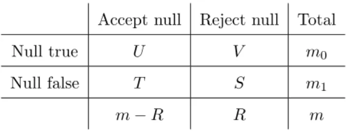
to control a global error related in some sense to the typeI errors that can occur. Table 1.1
shows all possible outcomes from a multiple testing procedure and suggests a variety of global error measures which could be controlled in practice. Most traditional methods aim to control the
quantityP(V ≥1), that is a multiple testing global error measure correspondent to thetype I error
rate in the single hypothesis testing set up. It is called Family Wise Error Rate (F W ER), and it
is the probability of obtaining at least on false positive.
In general, several techniques and different approaches have been proposed regarding the kind 9
Accept null Reject null Total
Null true U V m0
Null false T S m1
m−R R m
Table 1.1: Possible outcomes from testing m null hypothesis
of error measure considered, the inferential approach to estimate or control it (see section 1.2), the interpretation of probability on which inference is based (see section 1.1), the particular context the multiple tests are conducted under. In this chapter we do not discuss multiple testing methods
in general, but just focus on methods for controlling the False Discovery Rate (F DR), a particular
global error measure that we believe fruitful in the case of study of spatial epidemiology under examination. Motivations for this choice are explained in chapter 2.
1.1
False Discovery Rate
In this work we shall focus on the False Discovery Rate, that is the proportion of false discoveries (or false positives, or number of null hypotheses wrongly rejected) among all the discoveries (or positives, or number of null hypotheses rejected):
F DR= V
R (1.1)
Note it is a random quantity (neither bayesian nor frequentist) where both numerator and denom-inator are unknown short of having determined a decision rule for rejecting null hypotheses. It is worth noting that the authors who introduced the False Discovery Rate (Benjamini and Hochberg,
1995) calledF DRthe quantityEVR. We will instead denoteF DRas simply the fraction between
false discoveries and discoveries, following the terminology of Genovese and Wassermann (2003).
The F DRas a global error measure is frequently employed in the field of microarray data analysis
where multiple comparison problems arises in the identification of differentially expressed genes among a large number of observed gene expressions.
Several authors introduced p-value based methods that ”adjust” the procedure for rejecting
hypotheses such that in average the expected F DR is lower than a pre-specified error (Benjamini
and Hochberg, 1995; Storey, 2002). We refer to such methods as “frequentists” since they control the expected value of such a global error, taking the expectation over repeated experiments. Other proposals follow a Bayesian perspective and consider the null hypotheses as random variables, taking the expectation over them conditionally on the observed data. We will not review the several
methods proposed in literature but focus primarily on the methods based on posterior probabilities
of the null hypothesis (see section 1.3) rather thanp-values (see section 1.2). For a methodological
review of Bayesian proposals see Berry and Hochberg (1999); for a decisional theoretical approach
see Muller et al. (2006), while for an application of the F DR estimation through a hierarchical
Bayesian modeling framework in microarray data see Newton et al. (2004) and Broet et al. (2004).
1.2
Frequentist methods
Traditional methods for addressingF DRcontrol are based on the knowledge ofp-values and make
use of frequentist arguments to demonstrate the control. Benjamini and Hochberg (1995) achieve
the control of the expectation of theF DRas defined in (1.1), i.e. E(F DR) =E VR. In Benjamini
and Hochberg (BH) procedure a control of E(F DR) is obtained by rejecting as many hypotheses
as possible such thatE(F DR) is lower than a pre-specified valueα. Suchp-value based procedure
allows for rejecting all null hypotheses for which pi≤tp−value≡p(j) where:
j=max 0≤i≤m:p(i)≤α i m , (1.2)
and 0≡p(0)< p(1) < ... < p(m) denote the orderedp-values. BH demonstrated that E(F DR)≤α
regardless of how many null hypotheses are true and regardless of the distribution of thep-values
under the alternative hypothesis.
Storey (2002) focus on a “conservative” estimation of the expected positive False Discovery
Rate (pF DR) given a thresholdtp−value:
pF DR=E V R|R >0 (1.3) A conservative estimation as intended by the author is such that:
E(pF DR\(tp−value))≥E(pF DR(tp−value)). (1.4)
There is here a change of perspective in that the control is achieved by estimation of thepF DR
for fixed monotonic rejection regions (or monotonic sets of p-values) rather than by prefixing the
level ofF DRand work out the rejection region as in BH procedure. Storey (2003) uses a Bayesian
argument for ruling out a non-parametric estimator for the pF DR conditional on tp−value. He
provides estimators of a quantity called q-value that can be work out for each observed p-value.
Briefly, the q-value* relative to a given p-value* corresponds to the pF DR estimates conditional
on the rejection of all p-values lower than p-value*; for details see Storey (2003). Thus, building
relative to the highest observed p-value. Storey also shows a connection between his method and
BH procedure, demonstrating that for the same level of F DR a higher number of null hypotheses
can be rejected, gaining hence more sensitivity. The method makes however stronger assumption than BH, the most relevant being assumptions which yields the “Bayesian interpretation” of the
pF DR (Storey, 2003). Suppose m identical hypothesis tests aiming to evaluate null hypotheses
{H0i, ..., H0m}are performed considering the summary statistics{z(y1), ..., z(ym)}and the rejection
region Γ. Let us assume that (z(yi), H0i), fori= 1, ..., m, are i.i.d. random variables with marginal
distribution:
[z(yi)|H0i] =H0i·F0+ (1−H0i)·F1 (1.5)
whereF0andF1are the distributions ofz(yi) respectively under the null and alternative hypothesis,
and H0i ∼Bernoulli(prH0). Then it follows that:
pF DR(Γ) =P(H0i= 1|z(yi)∈Γ) (1.6)
(the notation [a|b] to mean the distribution of the random variable aconditional onbwill be used
in the following mostly when analytic expressions are introduced; when a more compact notation
helps the comprehension we will use the classic ∼).
The result holds for alli= 1, ..., mand regardless ofm. Moreover it is valid even if we consider
p-values instead of summary statistics. Storey proposed non-parametric estimators of pF DR(Γ)
by stressing the reasonable assumption that p-values distribution under H0 is U nif orm(0,1) so
achieving an estimator for the overall probability of the null hypothesis (calculated over the whole set of tests). The attempt to estimate such an overall probability is what allows the gain in power with respect to the BH procedure. In fact, considering a generalization of the BH result (Genovese
and Wasserman, 2003) we see that the BH procedure assures that E(F DR) ≤a·α ≤α, where a
is the overall probability of the null hypothesis, that is implicitly equal to 1 in the BH procedure.
Indeed, in the case where thepF DRestimator is obtained by using the most conservative estimation
of the overall probability of the null hypothesis (i.e. a = 1), BH procedure and Storey’s method
are equivalent.
1.3
Bayesian methods
The F DR is a ratio where both the numerator and the denominator depend on a decision about
the set of null hypotheses. We can generally define such a decision rule for H0i with the indicator
SupposeH0i = 1 indicates the unknown null hypothesis is true andH0i = 0 that the alternative
is true, hence the true F DRcan be formally expressed by:
F DR=
P
iH0i·di
D (1.7)
whereD=P
idi and di = 1 if the decision rule is such that H0i is rejected. Frequentist methods
use decision rule of the formdi=I(z(yi)≤tz), hence based on a summary statisticsz(yi) of data
and a critical valuetz. Decision rules of this form (or equivalently based onp-values) are intuitive
but not necessarily optimal as observed by Muller et al. (2006).
The Bayesian methods we will focus on consider H0i a binary random variable (equal to 1
when it is true) and allow us to determine the decision on theith null hypothesis by the posterior
probability that the null hypothesis itself is true, that is:
πi=P(H0i= 1|data) =E(H0i|data). (1.8)
note this quantity is conditional on the observed data. Muller et al. (2006) discusses decision rules
of the formdi(πi, tπ).
Considering frequentist expectation of the F DR, i.e. expectation over hypothetically repeated
experiments, we need to consider expectation over a ratio of random variables since the decision
di(z(yi)) is a function of the data and appears in both numerator and denominator of the ratio.
Under a Bayesian perspective the discussion simplifies because, looking at (1.7), the only unknown
quantity is the unknown H0i in the numerator, D being determined by a decision rule di(πi, tπ)
that is conditional on data. The F DR here is a function of the πi’s (and of a threshold tπ for
the πi’s) which are posterior probabilities conditional on the observed data. Thus, considering
each conditional expected value of H0i, i.e theπi’s defined in (1.8), we derive the expected F DR
conditional on data by:
E(F DR|data) =
P
iπid(πi < tπ)
D (1.9)
where the expectation is relative toH0i. This quantity is often used for addressing multiple
compar-isons problems in microarray data analysis. Following the mixture assumption of Storey (1.5) and introducing exchangeability (instead of i.i.d.) assumption on summary statistics, authors (Newton et al., 2004; Broet et al., 2004) proposed fully hierarchical Bayesian models for estimating the
expected F DR conditional on data. Such models can provide an estimate of each πi via MCMC
computation as a Monte Carlo mean over a sample of realizations from the respective posterior
distribution [H0i|data]. Given the estimatesπbi’s, an estimate of the expectedF DR conditional on
data is provided for any set of discoveries of cardinalityD by:
\
E(F DR|data) =
P
iπbid(πi < tπ)
As suggested in Newton et al. (2004), an estimate of the expected F DR conditional on data can be a suitable way to determine a decision function. Indeed, one can declare a null
hypoth-esis as rejected if πi < tπ∗, where tπ∗ is fixed to achieve a certain pre-set estimated F DR, say
\
E(F DR|data) ≥ c. Moreover, the authors observed the dual role of πbi in decision rules like
di(πbi, tπ). It not only determines the decision on H0i but also reports both the probability of a
false discovery as πbi, ifdi = 1, and the probability a false non-discovery as 1−πbi, ifdi= 0.
We will talk in more detail of these concepts in sections 3.2 and 3.2.1 when introducing and discussing the model proposed to address the case of study under exam.
1.3.1 Posterior probability adjustment for multiple testing
Estimating the posterior probability that the null hypothesis is true underlies considering the
null hypothesis H0i as a random variable rather than an unknown fixed parameter. Berry and
Hochberg (1999) observed “Posterior inference adjusts for multiplicities, and no further adjustment
is required”. The statement is true provided the assuming a probabilistic model for the null
hypotheses. First, the probability model needs to include a positive prior probability for the event “null hypothesis is true”. Second, the model needs to include a hyperparameter that defines the prior probability mass for all null hypotheses themselves. Moreover they comment that “finding posterior distribution of parameters is only part of the Bayesian solution. The reminder involves decision analysis”. Paper of Muller et al. (2006) discusses such a decision theoretical perspective
and derive optimal decision rules based on theπi’s under several loss functions dependent onF DR
and F N R (the False Non Discovery Rate). The optimal rule, determined by minimizing expected
F DR conditional on data, is of the form di =I(πi < tπ), where tπ can be analytically determined
under several loss functions.
To sum up, a full Bayesian hierarchical modeling is required to achieve what Berry and Hochberg called a posterior probabilities adjustment. The underlying idea of a fully Bayesian approach is
evaluating the ith test by means of πi, i.e. the ith posterior probability, but exploiting a Bayesian
shrinkage estimation such that all observations (not only ith observation) contribute to estimate
πi. Thus, the posterior distribution ofπi will depend on all the observed data, not only on the ith
Multiple testing on large datasets of
Standardized Mortality Ratios
Multiple testing in epidemiological applications is not always considered a primary issue. Some
authors deny the adoption of procedures to account for F W ER(Rothman and Greenland, 1998),
others advocate the control of it in epidemiological surveillance applications (Fris´en, 2003; Kulldorff,
2001; Elliott et al., 2000), though it has been noticed the cost in sensitivity of adopting the control ofF W ERin on-line monitoring (Rolka et al., 2007). It seems clear that multiple testing issues have to be considered in relation to a particular application. An important issue to carefully evaluate is the choice of the particular global error measure (see table 1.1 in chapter 1) to control/estimate in each particular case study. In this work we do not want to discuss multiple testing control from a theoretical point of view and claim it is necessary in the example we will introduce in this chapter, but we want to show that it can be viewed as a possible way to conduct a descriptive analysis of geographical epidemiology starting from the collection of many disease indicators. We shall describe a common spatial epidemiological example, its main features, its objectives and the statistical issues which arise. Then, in chapter 3, we shall attempt to build a multiple testing
procedure for it by means of a Bayesian hierarchical model that allows for estimating the F DR.
We will give reasons why this can be thought of as an interesting alternative to address a descriptive geographical epidemiological analysis, mostly in cases where data are over-dispersed and spatially correlated.
Firstly we introduce the epidemiological case under study and give some examples of its possible objectives in practice. Briefly, a descriptive analysis of Standardized Mortality or Morbidity Ratios
(SM R), collected in many areas, is undertaken to identify unusually high risks. The aim is to screen
the health status of area-specific populations, to identify priority for public health interventions or to suggest further analytical studies. For instance, an epidemiologist could be asked to look
at the difference in rates among the areas and attempt a ranking of higher-risk areas in order to allocate resources for public health administrative objectives (Greenland and Robins, 1991). Another example is the mapping of risk indicators relative to some disease of interest; here the scope is to describe the spatial distribution of the disease and to get clues about a possible association between the disease itself and the exposure to environmental risk factors. Moreover, a preliminary analysis can be done to detect clusters of one or more diseases under evaluation. For instance, one could test for the randomness of any pattern that can be found across areas, or screen for evidence of an individual disease hot spot (without any preconception about its likely location); the former are called tests for clustering and the latter tests for the detection of clusters (Besag and Newell, 1991). Thus, we see the range of preliminary statistical tools can be large and cannot be discussed here, just consider that, in general, methods use many different statistical inferential approaches according to their specific objectives and data features; see (Lawson et al., 1999) for a review of statistical methodologies available for addressing geographical analysis and some interesting remarks about their appropriateness in guiding public health policy decisions.
Among the examples above mentioned we will only discuss Bayesian disease mapping models, i.e. methods that give smoothed point estimates of risks in each area of the map considered. We would like to point out that both disease mapping models and the methodology proposed here to perform a multiple testing procedure controlling the FDR are only suitable for an analysis that may form the basis for subsequent epidemiologic investigations but will rarely be an end in themselves. In this work, the kind of preliminary analysis we will pursue is about testing each area-specific risk for a disease of interest (or more diseases that have the effect of augmenting the number of tests) being aware of the proportion of unusual high risks that more likely may have originated by chance. As regards the importance of the scale to which the events disease can be recorded, we can distinguish data collected at count (areal data) or point (case-event data) level, the former being our focus. For areal data analysis what is very relevant is the level of aggregation, i.e. if we have small or big spatial regions in the map under study. Often counts aggregated in small areas produces a zero count, a situation denoting data sparseness. An area is called small when a small count of disease events is expected inside it (sometimes the expected count is even lower than 1); this can either be due to the rarity of the disease under examination or because of the small number of people living there. The presence of small areas is one of the two main challenging issues we want to focus on, the second being the presence of spatial correlation between the risks.
In section 2.1 we give reasons for addressing an epidemiological descriptive analysis by means of a a multiple testing procedure on Standardized Mortality Ratios collected in many regions. We do not loose generality if we have many disease indicators collected in many areas. In section 2.3
we introduce the multiple hypothesis testing framework
To sum up, in this chapter we pose the ground for introducing a method to estimate the False Discovery Rate and controlling the multiple testing error, arguments discussed in chapter
3. We also consider p-value based control methods and claim their inappropriateness for several
reasons. Hence, we propose to estimate the F DR by using a methodology developed through a
well known disease mapping model (Besag et al., 1991) that is flexible as regards problems due to small areas and spatial correlation. We will also note that, in principle, the proposed model is able
to address both the F DR estimation relative to any possible set of rejected hypotheses and the
point estimation of true relative risk values.
2.1
The rationale of the work
Epidemiological studies aiming to identify unusually higher risks for one or more diseases over a map of geographic areas are denoted as descriptive studies even if the methods involved in such analysis often stress complex modelling assumptions. The general aim is to screen the health status of each area population by means of suitable disease indicators to identify risk increments for the examined diseases. Analyses are usually carried out on a predefined number of areas at a national, regional, or municipality level. The case we are focusing on is when a number of indicators are available collected in many regions, producing a large dataset. We also consider the presence of small areas over the map. Starting with the knowledge of such large datasets we want to highlight as many anomalies as possible, controlling some sort of measure which inform us about the anomalies that are imputable to only random error. Moreover, we would like to be able to evaluate the magnitude of risks in the areas declared as possibly at high-risk.
A well suited motivating example can be found in Catelan and Biggeri (2008), where authors pursue a statistical approach to rank multiple priorities in a case of study of environmental epi-demiology. They mention the control of the positive-False Discovery Rate like in Storey (2003) as a possible approach to such a case study. Our work is in the same direction as regards the epidemiological rationale, that is finding discoveries, or in other words, providing clues of which indicators are susceptible to represent high-risk situations, these being the priorities of investigation in a perspective of a preliminary and explorative statistical tool for epidemiologists. On this note someone may argue that controlling the False Discovery Rate determines a decision-oriented ap-proach which, traditionally, is not at all representative of a standard descriptive analysis. However, we think in such a case study a testing framework can still be though of as only addressing a pre-liminary statistical analysis since “descriptive” in this epidemiologic field does not strictly mean an analysis carried out by only summarizing empiric observations. Furthermore, the “ecology fallacy”
that typically affects such kind of aggregate indicators, limits conclusions that can be worked out by them, and makes such analyses advisable just at a preliminary stage (Lawson et al., 1999). Indeed, the further investigations aiming to confirm hypotheses generated by a descriptive analysis are, in the field of epidemiology, expensive observational studies (cohort studies, case control studies) conducted at an individual level. Thus, a decision based approach based on testing and control
the F DR on observed areal disease indicators cannot be considered a statistical tool finalized to
confirm the presence of environmental risk factors in those areas highlighted as at high-risk. It can, at most, generate hypothesis to further investigate through observational individual level studies.
2.1.1 The small areas issue
The recent availability of geographical indexed health and population data, together with advances in geographic information systems, has encouraged the epidemiological analysis on a small geo-graphic scale. A lot of issues arise with data collected in small areas in epidemiological applications of spatial statistics (Elliott et al., 2000). Some motivations are built around the increasing inter-pretability of small-scale studies, as they are less affected, in principle, by the ecology bias due to aggregating counts in areas that are heterogenous about the exposure to environmental factors (within area clusters presence is less probable if counts are aggregated at a small-scale). Conversely, small-scale studies require more sophisticated statistical techniques because the data are usually sparse with low (even zero) counts of events in most of the regions; a situation of data sparseness may still arise in large-scale studies when the disease is very rare. Furthermore, there is often evidence of over-dispersion of the counts with respect to the typically assumed Poisson model (see section 2.3.3) as well as spatial patterns indicating dependence between area-specific risks, both reasons making it suitable to approach the analysis by following the Bayesian hierarchical model paradigm. More details about the implications of the over-dispersion in the case under study can be found in section 2.3.3
2.1.2 The inferential approach
There are two main reasons why we undertake a Bayesian paradigm. First, data frequently encoun-tered in practice are in the form of large datasets of disease indicators collected at a small-scale, with underlying disease relative risks being spatially correlated across areas, both issues represent-ing statistical challenge well addressed by means of full Bayesian hierarchical models. The second reason arises from the inferential approach we want to undertake for addressing an analysis of such a large dataset, that is a multiple testing procedure controlling a particular multiple testing
in microarray data analysis for the selection of differentially expressed genes (Newton et al., 2004; Broet et al., 2004). Common features between the microarray context and our case study lies in the fact that a strict control is not recommended, the identification of as many as possible anomalies being the main interest. The main change of perspective lies in considering the null hypothesis as a random variable rather than a fixed unknown parameter. As a result, for the Bayesian statistician,
the inferential target will be the posterior probabilityπi of each area-specific null hypothesis (1.8)
rather thanp-values.
As said, our approach is decision-oriented, that is we want to make inference on a lot of null hypotheses since we are mostly interested in a method to actually provide rules for deciding which areas can be claimed high-risk areas, i.e. finding a rule for rejecting the null hypothesis, or for selecting discoveries in Benjamini Hochberg terminology. The reason why we propose a model for
estimating theF DR is that controlling the F DRin our case would mean measuring the error we
incur in selecting high-risk areas, so that, for any given set of rejected hypotheses we obtain an
inferential tool to estimate theF DR. However, to be able to determine a selection rule we still need
to change perspective: we need a method which, fixing a desiredF DRlevel, makes us able to select
as many high-risk areas as possible, or discoveries, being sure that the expected F DR would not
be greater than what is a priori pre-specified. We saw in chapter 1 that the Benjamini-Hochberg
procedure assures this under independence of p-values, whereas Storey builds a more powerful
method by means of more complex assumptions. We can say in advance that such methods are inappropriate when data show spatial correlation and over-dispersion (see section 2.3).
In chapter 3 we will discuss a model for estimating F DR overcoming in part the mentioned
difficulties. We will also discuss a way to determine selection rules based on the knowledge of the
estimatedF DRfor any set of areas declared at high-risk. As long as the model is good at estimating
theF DR, we can be reasonably certain in claiming a given number of discoveries at the pre-chosen
level of F DR. We can think of such a pre-chosenF DR level as a nominal value that the model
aims to predict. Thus, the reliability of such a kind of rule will be dependent on the ability of the
model to accurately estimate theF DR, especially avoiding under-estimation in order to achieve a
conservative control (similarly to the Storey’s perspective (1.4)). In chapter 4 we will discuss about
the spatial contexts, frequently met in practice, where the model can achieve conservative F DR
estimation. Moreover in chapter 4 we shall regard theF DRestimation capability as an interesting
way to determine a “non-arbitrary” rule for selecting high-risk areas. However, it is worth being
aware of the lack of sensitivity or specificity that such rules may yield for some F DR (nominal)
values; see section 4.4.
making statements about many hypotheses of absence of risk evaluated in small areas. We recall that the idea of selecting possible high-risk areas is of some sort of interest in epidemiology and some authors have suggested rules focused to this aim. For instance, Richardson et al. (2004) proposed to base a rule on the posterior probability that the relative risk is greater than 1. After a large simulation study a value of 0.8 came out as more appropriate in most spatial scenarios evaluated. Evaluating the posterior density placed in the right tail beyond 1 can be useful information, even if the goodness of such a rule is conditional on what value is chosen for the threshold (0.8 or another value?). Thus, unfortunately such a rule needs an arbitrary choice by the practitioner; a choice whose effect in terms of error produced in declaring high-risk areas cannot be known (because the object which the rule is based on, i.e. the posterior density, is an estimate of the true relative risk
value and there is no point in controlling a measure connected to the number of Type I errors).
With the rules suggested in chapter 3 a threshold for the F DR needs to be chosen, hence making
the practitioner aware of the number of errors he could at most incur. So, the only arbitrariness
introduced is the choice of the F DR level, analogous in some sense to choose the size α for a test
built with the Neyman-Pearson lemma. However, the goodness of the rule suggested still depends
on the accuracy of the F DR estimation which the model proposed is demanded.
2.2
Standardized Mortality or Morbidity Ratios
It is usual to assess the disease risk in a map of contiguous regions by collecting the observed
counts and calculating the expected counts. The ratio of observed to expected counts within
tracts is called Standardized Mortality/Morbidity Ratios (SMR) and this ratio is an estimate of “relative risk” within each tract (i.e. the ratio describes the relative risk of being in the disease group rather than the background group). Such indicators are easy to compute and often used in geographical epidemiology studies and also in contexts not involving spatial issues like occupational epidemiology (Tsai et al., 1986). Part of the section 2.3 focuses on the issues which arise employing such indicators for testing null hypotheses in such a case study. We shall discuss characteristics of a multiple testing setting based on such indicators, then we will recognize the inappropriateness
of frequentist p-value based methods for several reasons and claim the usefulness of a Bayesian
hierarchical approach.
We now define the likelihood model from which SM Rs can be worked out as maximum
like-lihood estimators. We assume the disease occurrence is available in the form of count of cases over a map of spatial regions. Small areas are those where we expect a small number of cases
because of the size of the area itself or the rarity of the disease. Within a map of N areas (census
expected count and the unknown relative risk in areai. It is usual to stress an i.i.d. Poisson model for observed counts:
Yi ∼P oisson(ei·ri) (2.1)
Thus, the likelihood of the relative risks ri is:
[yi|ei] = exp(−ei·ri)·
(ei·ri)yi
yi!
(2.2)
Here and in the following, the notation [a|b] generically denotes the conditional distribution of
agiven b. Similarly [a] will denote the marginal distribution of a.
The maximum likelihood estimator forriis actually the Standardized Mortality Ratio observed
in areai: b ri=SM Ri = yi ei (2.3)
The termei, that informs us about the area size, is assumed as known although it cannot actually be
observed, but it depends on some underlying assumptions about the population at risk underlying the map. Operatively, it can be worked out after having stratified the population at risk by age groups (or age-sex groups) and assuming a multiplicative model for such age group risks. Stratifying
is useful to make allowance for possible confounders. Since we want theSM Ri to be an indicator
of the association between the disease in question and the environmental exposure in area i, we
would like to get rid of all other possible variables that could modify (“confound”) the actual
environmental exposure of people in areai. For instance, older people may be thought to be more
exposed than younger people to a given disease, or, some disease may be more dangerous for males
than for females. We want the latter variables, age and sex, not to affect the SM Ri as we need
such indicators to inform us on only the risk associated with living in area i, regardless of if the
residents in areaiare exposed to any other risk factors (age and sex in this case) not under study.
In other words we might know that age and sex are important etiological factors for the disease of interest but in such an analysis we only want to focus on environmental factors. With this aim we can proceed by applying two indirect standardization methods: 1) a standardization using internal reference rates; 2) a standardization using reference rates of a standard external population. In the latter case we have:
ei =
X
j
Pij·qj
where qj is the disease rate in age group j for the reference population and Pij are the observed
person-years at risk in areaifor age groupj(the number of persons in age groupjwho live in area
assumed that the risk associated in living in area i(ri) acts proportionally on the baseline risk for
each strata (qj), hence:
qij =ri·qj (2.4)
Without introducing the latter assumption we propose propose a model for each age group observed count (Pascutto et al., 2000):
Yij ∼P oisson(Pij·qij)
However, the summation over the jth age groups in the (2.4) plus the assumption (2.4) lead
directly to model 2.1 where the count in area i is distributed as Poisson with mean (ei·ri). The
multiplicative model 2.4 is suitable as it allows for easily computing each areaiexpected count (ei)
that is the count of disease events we would expect if the disease rate in area iwere equal to that
of the standard population. Underlying ei there is already an idea of null hypothesis; see section
2.3. Model with a combination of an additive and a multiplicative effect has also been proposed in literature (Best et al., 2000).
In the internal standardization case we use as reference rates those of the population of the whole map, hence:
qj =
X
i
yij
Pij
Thus, this method centers the data as P
iei =
P
iyi and the overall mean disease rate is equal
to 1. It is the most used standardization method because it requires only the observed data. The external standardization, instead, builds expected counts consistent with the mean disease rate of another population assumed as a reference; i.e. a population supposed not to be exposed to the same environmental risk factors under study. Using one instead of the other standardization makes
a difference in the following sense: with internal standardization we will obtainSM Rs greater than
1 (constant mean rate), but also lower than 1, so adopting it we can describe the internal variability of disease rates. With external standardization, data are not constrained to the observed/expected
equivalence over summation (P
iei =
P
iyi) hence we can still obtain all disease rates greater or
lower than 1, because 1 in this case is not the constant mean rate.
There are two other assumptions underlying model 2.1. The first concerns the Poisson
proba-bility distribution: in each area i, individual risk levels are independent of each other, that is the
susceptibility to the disease is the same for all people living in that area. The second regards the independence and identity assumption (i.i.d.): counts of disease have no spatial correlation. In general, deviations from such assumptions yield counts more variable than what is expected under the Poisson model. This situation is commonly referred as over-dispersion, that is when the em-pirical variance of the data is larger than the variance specified by the model assumed to describe
the data. Typically it is assumed that the Poisson model is appropriate for rare and non infectious disease, though care should still be take about the level of aggregation of the disease events in counts, and the differences yielded by considering a regular grid or a real map with diverse area shapes; see further considerations on Poisson lack of fitting in section 2.3.3.
2.3
The multiple testing framework
Since we want to highlight unusually high relative risks we need many one tailed tests of hypothesis where the alternative hypothesis is that of higher relative risk value. Hence the two competing hypotheses are of the form:
H0i :ri = 1 (2.5)
H1i :ri >1 (2.6)
As we shall see in section 2.3.1 ap-value can be computed under the model whereYiis distributed
as the Poisson of meanei by calculating the c.d.f. of such Poisson distribution.
It is worth mentioning now that when we set up the model for estimating theF DR(see chapter
3) we will consider the simple null hypothesis r = 1 which makes the model specification easier.
Anyway, we want to say in advance that a complication will be met: a small posterior probability
πi can arise either in case where areairisk is lower or greater than 1. Hence, the practitioner, after
having computed posterior probabilities for all areas, will have to work out the F DR estimation
by only considering the set of the πi’s relative to areas eligible as possible discoveries (or possible
high-risk areas). We will consider as eligible for becoming discoveries the areas where the observed is greater than the expected count.
If the inferential aim is to conduct an hypothesis test in each of theN areas the multiple testing
problem ought to be addressed. In fact, doing a lot of tests we could incur wrong rejections making
necessary control of a global error measure. We have decided to control theF DRaiming to provide
information about how many False Discoveries we can expect, where a set of discoveries is defined as the set of areas that, by means of the decision rule, we can declare as being at high-risk.
As regards the choice of which multiple testing error control in such case we agree with authors
that advocate the False Discovery Rate as a more appropriate measure than theF W ERin all cases
where we need to find as many effects as possible (clues, anomalies etc.) in the dataset. As already mentioned in this chapter, this is consistent with a descriptive analysis aimed at screening disease indicators in an exploratory fashion rather than in a confirmatory study perspective, exactly like our
since we could reasonably let ourselves make even more than one error in declaring rejections; in other words, the decision to conduct more epidemiological investigations (on the whole map under study) need not be erroneous even if more than one null hypothesis is falsely rejected. Indeed, the
control of F W ERby a Bonferroni adjustment would yield a lot of false non-discoveries as it is very
conservative with respect to the null hypothesis. Moreover, the decision to keep on investigating with further high-cost epidemiological studies can not only be connected to this kind of geographical
analysis because they are not free of troubles. Such SM Rs analyses stand at the lowest level of
proof about confirming etiological effects due to exposure to environmental risk factors because of the “ecology fallacy” and many other possible confounders unobserved at area level. The analysis is only required to throw light on possible anomalies. On this note, providing a method to estimate
theF DR given a number of discoveries is a possible way to proceed. If, moreover, the method can
estimate both false discoveries and relative risk values (i.e. the magnitude of the discoveries) it may probably be viewed as a more informative way than merely plotting relative risk values on a map or ranking high-risk areas. The model proposed in chapter 3 is indeed aimed at both estimating
F DR and relative risks.
As an example, Biggeri et al. (2007) applied Storey pF DR estimators to achieve q-values
relative to disease indicators tested in some areas of Sardinia and observed the usefulness of the False Discovery Rate to asses the global degree of risk of a given area where more than one indicator was available (several causes of disease under examination). For each area they were able to select
some discoveries at the level of F DR (indeed the pF DR) indicated by the q-value correspondent
to each p-value. The limitation here is that aq-value (i.e. an estimation of the proportion of false
discoveries) can be computed for only ordered sets of p-values (also denoted asp-value monotonic
sets). We believe the F DR is a useful measure also for our case study, that is slightly different as
we aim to make test on SM Rs collected in small and contiguous areas and also addressing case
where risks show positive spatial correlation. As we will see in section 2.3.2 in our mind a small
area is when the expected count ei is lower than 5.
In the following we shall approach the methodology applied for estimating theF DRgradually.
Firstly we will mention related arguments like the mapping issue, the interpretation of the
over-dispersion as regards the null and alternative hypothesis and ways for computing a p-value for
testing an SM R.
2.3.1 Mapping significance or mapping Relative risks
Producing maps of indicators telling us about the disease under examination is a primary aim of any descriptive analysis based on disease counts collected in many areas. A lot of authors have
noted the difficulty in interpreting maps of SM Rs (Cressie, 1993; Banerjee et al., 2004; Gelman
and Price, 1999; Molli´e, 1996; Elliott et al., 2000; Pascutto et al., 2000; Schlattmann et al., 1993)
when the population underlying the areas is heterogeneous and mostly when some counts arise by counting events in poorly sampled areas. Poorly sampled areas are actually the small areas, those
where the expected count is very small (even lower than 1) hence yielding a large SM R. Because
of small areas the map will show a discontinuity in estimated rates since low expected count areas
could yield a huge SM R for the occurrence of only a few cases of disease. On the other hand
such estimates will be very inaccurate since the standard error ofSRMi depends on the population
living in areai, precisely:
b sd(SM Ri) = √ yi ei (2.7)
whereei, as known, gives a clue about the area size. To sum up, mapping the SM Rs(sometimes
called crude rates) will actually highlight high risks only in small areas. Disease mapping models address such problems allowing us to work out adjusted estimates of the true relative risk values,
smoothed with respect to theSM Rs.
We want to attempt to set a hypothesis test for each area (region) of the map. In literature we
can find a few examples that underly the idea of testing hypotheses on the collectedSM Rsrather
than pursuing the inferential goal of estimating the relative risk values. As an example, Cressie
(1993), quoting an earlier work of Choynowski (1959), considers a map of p-values of the form:
pi = 1−P(Yi ≤yi |H0i :Yi ∼P oisson(ei)) ei ≤yi P(Yi < yi |H0i:Yi ∼P oisson(ei)) ei ≥yi
where recallyi and ei are both known values; the former being empirically observed and the latter
being computed by introducing assumptions discussed in section 2.3. By Analyzing the North Carolina Sudden Infant Death Syndrome (SIDS) dataset, where for 100 counties counts of numbers
of live births and numbers of sudden infant deaths are available, Cressie, as regards the p-values
computed as above, observed as “an extreme value . . . may be more due to its lack of fitting to Poisson model than to its deviation from the constant rate assumption”. Recall that the constant rate assumption in our setting corresponds to the null hypothesis (2.5).
In Shlattmann (1993) there is the idea of assigning area to high risk groups. The method aims to estimate the heterogeneity in relative risks, another issue that is typically pursued preliminarily
to the construction of maps of disease. This is when we can reject the hypothesis that yi ∼
P oisson(ei ·r) in favor of the alternative yi ∼ P oisson(ei ·ri), i.e. that relative risks are not
its importance and noting that a Bonferroni adjustment on Poisson p-values, besides leading to a dramatic loss of power, is unable to provide a consistent estimate of the proportion of true null hypothesis either. However, the mixture modeling approach for disease mapping proposed by
Schlattmann may potentially represent a useful ground for inclusion of F DR estimation.
2.3.2 P-values computation in small areas
Frequentist methods to control/estimate theF DRare based on the knowledge of onlyp-values. In
order to assess the possibility to apply such methods we try to find a suitable p-value for evaluating
the null hypothesis of absence of risk. Following the hypothesis testing setting in section 2.3 we
could consider each ith area-specific p-value of the form:
pi= 1−P(Yi ≤yi |H0i:ri= 1) (2.8)
Recall our interest is in an unilateral alternative hypothesis: a risk higher than what is expected.
Thus, in principle, extremely small p-values should occur in areas where the observed count is
unusually higher than the expected one. However, as Cressie (1993) noted evaluating the null
hypothesis with such kinds of p-value can lead to troubles when the disease outcome is rare or
areas are small. Moreover Molli´e (1996) have correctly noted that, while mappingSM Rshighlights
higher risk just in low-populated areas, significance maps can highlight unusual risks just in
high-populated areas, i. e. where the standard error of the SM R is small.
There are two main problems: first, ap-value calculated in a small expected count area, cannot
guarantee the same empiric evidence of ap-value computed in a bigger expected count area; second,
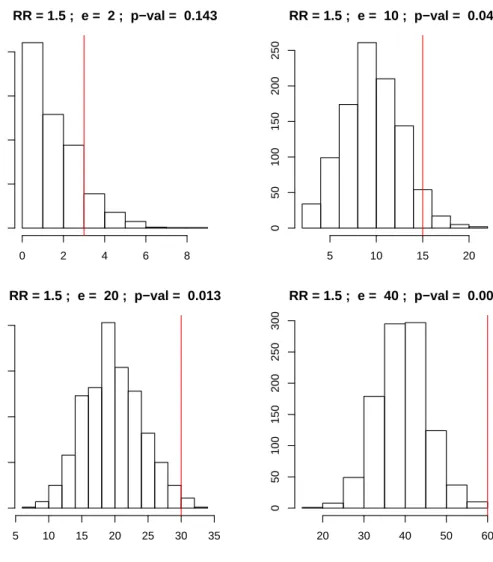
it can be shown via simulation that, for the same level of risk greater than 1 (as ex. r = 1.5, i.
e. a 50 % of risk increment compared with that expected), a p-value calculated in small expected
count areas is less extreme (i.e. more conservative) than one calculated in bigger expected count
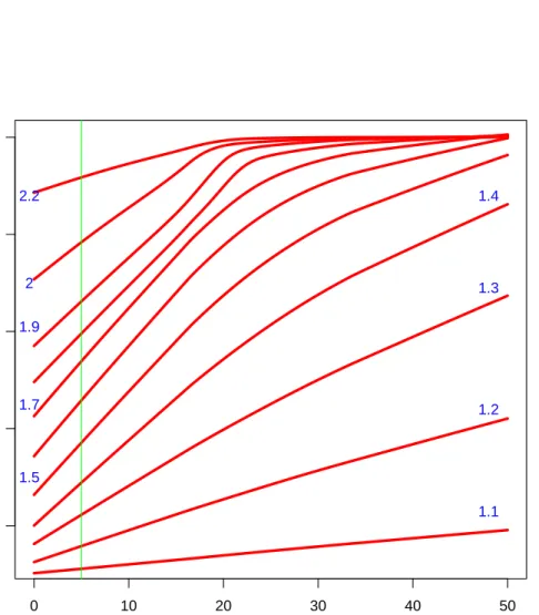
areas; see Figure 2.2. To sum up, we cannot trust each p-value to the same degree (first point),
and, even worse, tests evaluated with such p-value are powerless in poorly sampled areas (second
point). See Figure 2.1 which shows a plot of the power against the expected count level concerning several values of the alternative hypothesis.
Moreover, note the p-value computation involves the cumulative distribution function of the
following two ways to obtain ap-value: pi= 1−P(Yi ≤yi |ei) = 1− yi X k=0 exp(−ei)·eki k! (2.9) pi = 1−P(Yi< yi|ei) = 1− yi−1 X k=0 exp(−ei)·eki k! (2.10)
It is clear that whether or not including the observed valueyiin the summation makes a difference,
but such a difference is more emphasized in case where ei (the mean parameter of the Poisson
variable Yi) is a small value, i.e. in small areas. The small area p-values conservativeness is due
to the discrete distribution of the test statistics yi, that is indeed a count. Generally, with a
discrete distribution it is not possible to construct confidence intervals with specified coverage (the probability that the confidence interval contains the parameter of interest). Thus, one typically uses confidence intervals with the nominal coverage as the lower bound for the actual coverage.
This will result in conservative p-values and conservative confidence intervals, that is to say that
the significance level of the test is less and the coverage probability of the confidence interval is greater than nominal. This conservativeness is stronger in small areas, where the expected value of the Poisson distribution is small; see results obtained via simulation by Kulkami (1998).
The above described is just one of the possible ways to obtain a p-value for testing a count
having available an expected count as the true value under the null model. Some proposals of
p-value computation for testing an SM R have involved normal approximation for the log(SM R)
(Armitage, 1971; Banerjee et al., 2004) that, however, improves as long as the number of observed
deaths gets larger. Other authors have suggested methods exploiting the relation betweenχ2 and
Poisson distribution (Ulm, 1990) to calculate an exact confidence interval and find a p-value by
means of only a table of the χ2 distribution. Also non computer intensive algorithms that refine
the coverage, so achieving less conservativep-values, are available (Kulkami et al., 1998).
2.3.3 The Over-dispersion issue
Let us suppose to set up a multiple testing procedure by evaluating each area-specific test with
a p-value expressed as (2.8). In the next section we will focus on problems relative to applying
frequentistp-value based methods. Here we consider the over-dispersion case in relation top-values.
In previous sections we said that it is likely to find extreme p-values in areas with a large
population, conversely to mapping theSM Rsthat would highlight just small areas because of small
denominators. We also pointed out, quoting Cressie (1993), that extreme p-values may be more
due to a lack of fitting of the Poisson model than to an actual deviation from the null hypothesis
that the mean of the Poisson isei. Lack of fit of the Poisson model can be equivalently denoted as
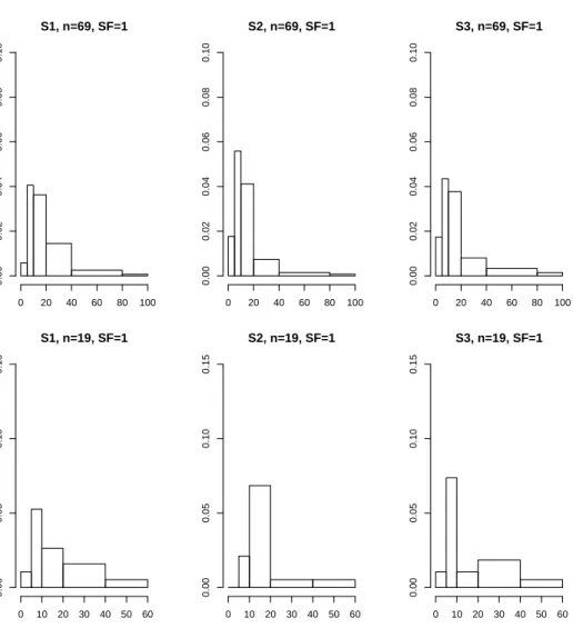
● ● ● ● ● ● ● ● ● ● ● ● ●● ● ● ● ● ● ● ● ● ●● ● ● ● ●● ● ● ●● ●● ●● ● ●● ●●● ●● ● ● ● ●● ●● ● ● ● ● ●● ● ● ● ● ● ●● ●● ● ● ● ● ● ●● ● ● ● ●● ● ● ● ● ●● ●● ● ●● ●● ● ●● ●●● ●●● ● ● ●● ●● ● ● ● ● ● ● ● ●● ● ● ● ● ● ●● ● ● ●●● ●●● ● ● ●● ●● ● ● ●● ●●● ●● ●●● ● ●● ●●●● ● ● ●● ● ●● ● ●● ●● ● ●● ● ● ● ●●● ● ● ●●●● ● ● ●●● ●● ● ● ● ●● ● ● ●● ● ●● ●●● ● ● ● ●● ●●● ● ●● ● ●● ● ●●●● ● ● ●● ● ● ●●● ● ●● ● ● ●● ●● ●● ● ●●● ●●● ●● ● ● ● ● ●● ●● ●●● ● ● ● ● ● ● ●●● ● ● ● ●●●●● ● ● ●● ●●●● ●●● ●● ●●●● ●●●● ●●●●● ● ● ●●●● ● ● ● ●●●● ● ●● ●● ●●●● ● ●●●●● ●● ● ●●●●●●● ● ●● ● ●●● ● ● ● ● ● ● ● ● ● ●●● ● ● ● ●●●● ● ● ●● ● ●● ●● ● ●● ● ● ●●● ●●● ● ●●●●●● ● ●●●●● ● ● ● ● ●●●●● ●●●● ●●● ● ●●●●●●● ●●●● ●● ●●● ● ●●●●●●●● ● ● ●●●●● ● ●● ● ●●●●●●●●●●● ●● ●●● ●● ●●●●●●●●●●●●●●●●●●●●●●● ●●● 0 10 20 30 40 50 0.2 0.4 0.6 0.8 1.0
size areas (expected count)
sensitivity 1.1 1.2 1.3 1.4 1.5 1.7 1.9 2 2.2
Figure 2.1: Power against size area. For each value of expected count (size area) in the horizontal
axis, we see plotted the sensitivity of the test that reject the null hypothesis (2.5) when the p
-value calculated with formula (2.8) is lower than 0.05. We also see that the sensitivity is generally lower in small areas case. Each line corresponds to several values (coloured blue) of the alternative
hypothesis (r >1) under which the power is calculated as the proportion of the times that the null
hypothesis is correctly rejected. The green line is in correspondence with an expected count of 5, a limit under which we arbitrarily consider an area to be small.
RR = 1.5 ; e = 2 ; p−val = 0.143 simulated counts Frequency 0 2 4 6 8 0 100 200 300 400 RR = 1.5 ; e = 10 ; p−val = 0.049 simulated counts Frequency 5 10 15 20 0 50 100 150 200 250 RR = 1.5 ; e = 20 ; p−val = 0.013 Frequency 5 10 15 20 25 30 35 0 50 100 150 200 RR = 1.5 ; e = 40 ; p−val = 0.001 Frequency 20 30 40 50 60 0 50 100 150 200 250 300
Figure 2.2: Histograms showingp-values obtained with formula (2.8) in four possible areas differing
for their expected count. The expected counts are 2, 10, 20, 40 and the observed counts (red line)
are respectively 3.5, 15, 30, 60 consistent with a relative risk constantly equal to 1.5. Thus, given
the same value for the relative risk, bigger areas show more extremep-values, hence yielding a more
be frequently encountered in the case of counts collected in small areas (Molli´e, 1996; Haining et al., 2008). Generally, for rare disease and for small areas, variation in the observed number of events exceeds that expected from Poisson inference. In a given area, variation in the number of events is due partly to Poisson sampling, but also due to extra-Poisson variation arising from variability in the disease rate within the area, which result from heterogeneity in individual risk levels within the area.
Heterogeneity of the individual risks can be due to spatial interaction effects at area level. Consider the case of infectious disease modelling where one individual having the disease raises the risk of infection for individuals in the same spatial unit. The consequence is a tendency for cases to cluster so that some areas have large counts (where the disease has started and spread) and some others have small, possibly zero, counts (where the infection has not yet arrived). The same effect can be created by unobserved environmental factors that operate at area level, determining non independent risk levels within the area. The presence of a pollution source, for instance, my have a non homogeneous effect for the whole inner-area population determining non independent individual risk levels. Moreover, though the classic standardization operation aims to eliminate the effect of confounding factors like age and sex, a variety of other unmeasured factors can influence the individual response. Thus, the inner-area heterogeneity can be due to a number of unobserved variables, such as lifestyle and genetic inheritance. To sum up, individual risk heterogeneity is to be expected when dealing with aggregates, especially of non-experimental subjects (like our case where we simply collect death events), and is a source of over-dispersion. Finally, if the scale of the spatial unit used to record the data is such that one of the above factors (environmental, social, or genetic), or simply the contagiousness of the disease, could also operate between the spatial units, it may induce positive spatial correlation in the counts too. The term positive (negative) spatial correlation refers to the property of attribute measured at nearby or adjacent geographical locations having similar (dissimilar) values. Thus, we can see as the invalidity of assumptions in the model (2.1), i.e. the i.i.d assumption and the mean-variance equality, is actually due to the lack of independence between individual underlying risks of people that can operate within areas or between areas.
To understand whether or not testing SM Rs for screening health population status with p
-values (2.8) is appropriate we should ask ourselves two things: if SM Rs can be appropriate for
evaluating the health status of a region, and if an extremep-value signals unusual risks. The former
question could be answered, as already discussed, saying that, though we can standardize for some
measurable confounders, we could never assume an SM R > 1 due to exposure to environment