(will be inserted by the editor)
Enhancing Regression Models for Complex Systems using
Evolutionary Techniques for Feature Engineering
Patricia Arroba · Jos´e L. Risco-Mart´ın · Marina Zapater · Jos´e M. Moya · Jos´e L. Ayala
Received: date / Accepted: date
Abstract This work proposes an automatic method-ology for modeling complex systems. Our methodmethod-ology is based on the combination of Grammatical Evolu-tion and classical regression to obtain an optimal set of features that take part of a linear and convex model. This technique provides both Feature Engineering and Symbolic Regression in order to infer accurate mod-els with no effort or designer’s expertise requirements. As advanced Cloud services are becoming mainstream, the contribution of data centers in the overall power consumption of modern cities is growing dramatically. These facilities consume from 10 to 100 times more power per square foot than typical office buildings. Mod-eling the power consumption for these infrastructures is crucial to anticipate the effects of aggressive opti-mization policies, but accurate and fast power model-ing is a complex challenge for high-end servers not yet satisfied by analytical approaches. For this case study, our methodology minimizes error in power prediction. This work has been tested using real Cloud applica-tions resulting on an average error in power estimation of 3.98%. Our work improves the possibilities of deriv-ing Cloud energy efficient policies in Cloud data centers
P. Arroba, J. M. Moya Electronic Engineering Dept.,
Technical University of Madrid, Madrid 28040, Spain E-mail:{parroba,josem}@die.upm.es
J. L. Risco-Mart´ın, J. L. Ayala
DACYA, Complutense University of Madrid, Madrid 28040, Spain
E-mail:{jlrisco,jayala}@ucm.es M. Zapater
CEI Campus Moncloa
UCM-UPM, Madrid 28040, Spain E-mail: [email protected]
being applicable to other computing environments with similar characteristics.
Keywords Automatic modeling·Complex Systems· Grammatical Evolution ·Classical regression ·Green data centers ·Sustainable Cloud computing · Power modeling
1 Introduction
Analytical models, as closed form solution represen-tations, require specific knowledge about the different contributions and their relationships, becoming hard and time-consuming techniques for describing complex systems. Complex systems comprise a high number of interacting variables, so the association between their components is hard to extract and understand as they have non-linearity characteristics [4]. Also, input pa-rameter limitations are barriers associated to classical modeling for these kind of problems.
Otherwise, classical regressions as least absolute shrink-age and selection operator techniques provide models with linearity, convexity and differentiability attributes, which are highly appreciated for describing systems per-formance. However, the automatic generation of accu-rate models for complex systems is a difficult challenge that designers have not yet fulfilled by using analytical approaches.
On the other hand, metaheuristics are higher-level procedures that make few assumptions about the opti-mization problem, providing adequately good solutions that could be based on fragmentary information [6, 7]. They are particularly useful in solving optimiza-tion problems that are noisy, irregular and change over time. In this way, metaheuristics appear as a suitable
approach to meet optimization problem requirements for complex systems.
Some metaheuristics, as Genetic Programming (GP), perform Feature Engineering (FE) that is a particu-larly useful technique for selecting an optimal set of features that best describe an optimization problem. Those features consist of measurable properties or ex-planatory variables of a phenomenon. FE methods se-lect adequate characteristics avoiding the inclusion of irrelevant parameters that reduce problem generaliza-tion [32]. Finding relevant features typically helps with prediction; but correlations and combinations of rep-resentative variables, also provided by FE, may offer a straightforward view of the problem thus generating better solutions.
Grammatical Evolution (GE) is an evolutionary com-putation technique based on GP. This technique is par-ticularly useful to solve optimization problems and pro-vides solutions that include non-linear terms offering FE capabilities that remove analytical modeling bar-riers. One of the main characteristics of GE is that it can be used to perform Symbolic Regression (SR) [29]. Also, designer’s expertise is not required to process a high volume of data as GE is an automatic method. However, GE provides a vast space of solutions that may be bounded to achieve algorithm efficiency.
In this work we propose a novel methodology for the automatic inference of accurate models that combines the benefits offered by both classic and evolutionary strategies. Firstly, SR performed by a GE algorithm finds optimal sets of features that best describe the system behavior. Then, a classic regression is used to solve our optimization problem using this set of features providing the model coefficients. Finally, our approach provides an accurate model that is linear, convex and derivative and also uses the optimal set of features. This methodology can be applied to a broad set of optimiza-tion problems of complex systems. This paper presents a case study for its application in the area of Cloud power modeling as it is a relevant challenge nowadays.
1.1 Motivation
One of the big challenges in data centers is the power-efficient management of system resources. Data centers consume from 10 to 100 times more power per square foot than typical office buildings [30] even consuming as much electricity as a city [23]. Consequently, a careful management of the power consumption in these infras-tructures is required to drive the Green Cloud comput-ing [11].
Cloud computing addresses the problem of costly computing infrastructures by providing dynamic resource
provision on a pay-as-you-go basis, and nowadays it is considered as a valid alternative to owned high perfor-mance computing (HPC) clusters. There are two main appealing incentives for this emerging paradigm: firstly, the Clouds’ utility-based usage model allows clients to pay per use, increasing the user satisfaction; secondly, there is only a relatively low investment required for the remote devices that access the Cloud resources [12].
Besides economic incentives, the Cloud model pro-vides also benefits from the environmental perspective, since the computing resources are managed by Cloud service providers but shared among all users, which in-creases their overall utilization [5]. This fact is trans-lated into a reduced carbon footprint per executed task, diminishingCO2emissions. The Schneider Electric’s
re-port on virtualization and Cloud computing efficiency [27] confirms that about 17% of annual savings in energy consumption were achieved by 2011 through virtualiza-tion technologies.
However, the proliferation of modern data centers is growing massively due to the current increase of appli-cations offered through the Cloud. A single data center, that houses the computer systems and resources needed to offer these services, has a power consumption com-parable to 25000 households [21]. As a consequence, the contribution of data centers in the overall consumption of modern cities is increasing dramatically. Therefore, minimizing the energy consumption of these infrastruc-tures is a major challenge to reduce both environmental and economic impact.
The management of energy-efficient techniques and aggressive optimization policies requires a reliable pre-diction of the effects caused by the different procedures throughout the data center. Server heterogeneity and diversity of data center configurations difficult to in-fer general models. Also, power dependency with non-traditional factors (like the static consumption and its dependence on temperature, among others) that affect consumption patterns of these facilities may be devised in order to achieve accurate power models.
These power models facilitate the analysis of several architectures from the perspective of the power con-sumption, and allow to devise efficient techniques for energy optimization. Data center designers have col-lided with the lack of accurate power models for the energy-efficient provisioning and the real-time manage-ment of the computing facilities. Therefore, a fast and accurate method is required to achieve overall power consumption prediction.
The work proposed in this paper makes substantial contributions in the area of power modeling of Cloud servers taking into account these factors. We envision a powerful method for the automatic identification of
fast and accurate power models that target high-end Cloud server architectures. Our methodology considers the main sources of power consumption as well as the architecture-dependent parameters that drive today’s most relevant optimization policies.
1.2 Contributions
Our work makes the following contributions:
– We propose a method for the automatic generation of fast and accurate models adapted to the behavior of complex systems.
– Resulting models include combination and correla-tion of variables due to the FE and SR performed by GE. Therefore, the models incorporate the op-timal selection of representative features that best describe system performance.
– Through the combination of GE and classical regres-sion provided by our approach, the inferred models have linearity, convexity and differentiability prop-erties.
– As a case study, different power models have been built and tested for a high-end server architecture running several real applications that can be com-monly found in nowadays’ Cloud data centers, achiev-ing low error when compared to real measurements. – Testing for different applications (web search en-gines, and both memory and CPU-intensive appli-cations) shows an average error of 3.98% in power estimation.
The remainder of this paper is organized as follows: Section 2 gives further information on the related work on this topic. Section 3 provides the background algo-rithms used for the model optimization. The methodol-ogy description is presented in Section 4. In Section 5 we provide a case study where our optimization modeling methodology is applied. Section 6 describes profusely the experimental results. Finally, in Section 7 the main conclusions are drawn.
2 Related Work
A complex system can be described as an intercon-nected agents system exhibiting a global behavior that results from agents interactions [8]. Nowadays, the num-ber of agents in a system grows in complexity, from data traffic scenarios to multisensor systems, as well as the possible interactions between them. Therefore, infering the global behavior, not imposed by a central controller, is a complex and time-consuming challenge
that requires a deep knowledge of the system perfor-mance. Due of these facts, new automatic techniques are required to facilitate the fast generation of models that are suitable for complex systems presenting a large number of variables.
The case study presented in this work exhibits high complexity in terms of number of variables and pos-sible traditional and non-traditional sources of power consumption. This issue demands the following review of the state-of-the-art.
In the last years, there has been a rising interest in developing simple techniques that provide basic power management for servers operating in a Cloud, i.e. turn-ing on and off servers, puttturn-ing them to sleep or us-ing Dynamic Voltage and Frequency Scalus-ing (DVFS) to adjust servers’ power states by reducing clock fre-quency. Many of these recent research works have fo-cused on reducing power consumption in cluster sys-tems [1], [35], [15], [20].
In general, these techniques take advantage of the fact that application performance can be adjusted to utilize idle time on the processor to save energy [13]. However, their application in Cloud servers is difficult to achieve in practice as the service provider usually over-provisions its power capacity to address worst case scenarios. This often results in either waste of power or severe under-utilization of resources. Thus, it is critical to quantitatively understand the relationship between power consumption, temperature and load at the sys-tem level by the development of a power model that helps in optimizing the use of the deployed Cloud ser-vices.
Currently the state-of-the-art offers various analyti-cal power models. However, these models are architecture-dependant and do not include the contribution of static power consumption, or the capability of switching the frequency modes (DVFS). The authors develop linear regression models that present the power consumption of a server as a linear function of its CPU usage [22], [28]. Some other models can be found where server power is formulated as a quadratic function of the CPU us-age [24], [34]. Still, as opposed to ours, these models do not include the estimation of the static power consump-tion (which has turned to have a great impact due to the current server technology).
Bohra et al. [9] propose a robust fitting to calcu-late their model that takes into account the correla-tion between the total system power consumpcorrela-tion and component utilization. Our work follows a similar ap-proach but also incorporates the contribution of the static power consumption, its dependence on tempera-ture, and the effect of applying voltage and frequency scaling techniques.
Interestingly, one key aspect in the management of a data center is still not very well understood: control-ling the ambient temperature at which the data cen-ter operates. Data cencen-ters operate in a broad temper-ature range from 18◦C to 24◦C but some can be as cold as 13◦C [10, 25]. However, due to the lack of ac-curate power models, the effect of ambient tempera-ture on the power consumption of the servers has not been clearly analyzed, preventing the application of op-timization models to save energy. On the contrary, the experimental work presented in this paper has been per-formed in ambient temperatures ranging from 18◦C to 25◦C. The range selected follows nowadays’ practice of operating at higher temperatures [17] and close to the limits recommended by ASHRAE. Although this prac-tice obtains energy savings in the cooling expense [14], the lack of a detailed power model prevents to apply optimization policies.
In our previous work, we have applied the benefits of Particle Swarm Optimization algorithms (PSO) to identify an analytical model that provides accurate re-sults for power estimation [2]. PSO simplifies the power model by significantly reducing the number of prede-fined parameters and variables used in the analytical formulation. However, as a parameter identification mech-anism, this technique does not provide an optimal search of the features that best describe the system power per-formance, so additional features could be incorporated.
The work presented in this paper outperforms pre-vious approaches in the area of power modeling for en-terprise servers in Cloud facilities in several aspects:
– Our approach consists on an automatic method for the identification of an accurate power model par-ticularized for each target architecture. We propose an extensive power model consistent with current architectures.
– The proposed methodology takes into account the main power consumption sources resulting in a mul-tiparametric model to allow the development of power optimization approaches. Different parameters are combined by Feature engineering assuring that the optimal set of features is considered.
– Optimal features are included in a classical regres-sion resulting in a specific model instance for ev-ery target architecture that is linear, convex and derivable. Also the execution of the resulting power model is fast, making it suitable for run-time opti-mization techniques.
3 Algorithm description 3.1 Grammatical Evolution
As previously stated, we work on FE to obtain mathe-matical expressions that represent different power con-sumption contributions. These expressions, or features, are derived from the combination of previously collected experimental parameters (in our case of study, they cor-respond to processor and memory temperatures, fan speeds, processor and memory utilizations, processor frequencies and voltages). We deal with a kind of SR problem to select the relevant features. SR tries to si-multaneously obtain a mathematical expression while including the relevant parameters to reproduce a set of discrete data. Besides, GP has proven to be effective in a number of SR problems [33]. However, GP presents some limitations like bloating of the evolution (exces-sive growth of memory computer structures), often pro-duced in the phenotype of the individual. During the last years, variants to GP like GE appeared as a simpler optimization process [26]. In our approach, GE allows the generation of a new set of optimized features by ap-plying SR. This feature generation is achieved thanks to the use of grammars that define the rules for obtaining mathematical expressions. More concretely, we will use grammars expressed in Backus Naur Form (BNF) [26]. A BNF specification is a set of derivation rules, ex-pressed in the form:
<symbol>::=<expression>
The rules are composed of sequences of terminals and non-terminals. Symbols that appear at the left are non-terminals while terminals never appear on a left side. In this case we can affirm that <symbol> is a non-terminal and, although this is not a complete BNF specification, we can affirm also that<expression>will be also a non-terminal, since those are always enclosed between the pair < >. Therefore, in this case the non-terminal<symbol>will be replaced (indicated::=) by an expression. The rest of the grammar must define the different alternatives.
A grammar is represented by the 4-tupleN, T, P, S, beingN the non-terminal set,T is the terminal set,P the production rules for the assignment of elements on N andT, andSis a start symbol that should appear in N. The options within a production rule are separated by a “|” symbol.
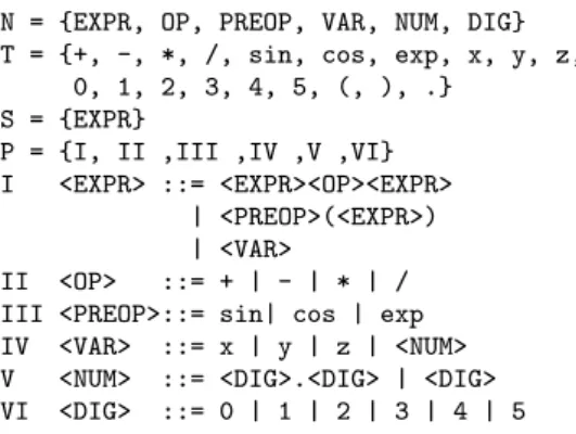
Figure 1 represents an example of a grammar in BNF, designed for symbolic regression. The final ob-tained expression will consist of elements of the set of terminalsT. These have been combined with the rules of the grammar, as explained previously. Also, gram-mars can be adapted to bias the search of the relevant
N = {EXPR, OP, PREOP, VAR, NUM, DIG} T = {+, -, *, /, sin, cos, exp, x, y, z,
0, 1, 2, 3, 4, 5, (, ), .} S = {EXPR}
P = {I, II ,III ,IV ,V ,VI} I <EXPR> ::= <EXPR><OP><EXPR>
| <PREOP>(<EXPR>) | <VAR>
II <OP> ::= + | - | * | / III <PREOP>::= sin| cos | exp IV <VAR> ::= x | y | z | <NUM> V <NUM> ::= <DIG>.<DIG> | <DIG> VI <DIG> ::= 0 | 1 | 2 | 3 | 4 | 5
Fig. 1 Example of a grammar in BNF format designed for symbolic regression
features because there is a finite number of options in each production rule.
Regarding both the structure and the internal op-erators, GE works exactly like a classic Genetic Algo-rithm (GA) [3]. GE evolves a population formed by a set of individuals, each one constituted by a chromosome and a fitness value. In SR, the fitness value is usually a regression metric like Root Mean Square Deviation (RMSD), Coefficient of Variation (CV), Mean Squared Error (MSE), etc. In GE, a chromosome is a string of integers. In the optimization process, GA operators named selection, crossover and mutation are iteratively applied to improve the fitness value of each individ-ual. In order to compute the fitness function for every iteration and to extract the mathematical expression given by an individual, a decoding process is applied. We refer the reader to [16] to understand the different GA operators. In the following, we explain through an example the decoding process performed in GE, since it clearly explains how better features are automati-cally selected. Let us suppose that we have the BNF grammar provided in Figure 1 and the following 7-gene chromosome:
21-64-17-62-38-254-2
According to Figure 1, the start symbol isS={EXPR}, hence the decoded expression will begin with this non-terminal:
Solution = <EXPR>
Now, we use the first gene of the chromosome (also called codon, equal to 21 in the example) in rule Iof the grammar. The number of choices in that rule is 3. Hence, a mapping function (the modulus operator) is applied:
21 MOD 3 = 0
and the first option is selected<EXPR><OP><EXPR>. The selected option substitutes the decoded non-terminal.
As a consequence, the current expression is the follow-ing:
Solution = <EXPR><OP><EXPR>
The process continues with the next codon, 64, which is used to decode the first non-terminal of the current ex-pression, namely,<EXPR>. Again, the mapping function is applied to ruleI:
64 MOD 3 = 1
and the second option<PREOP>(<EXPR>)is selected. So far, the current expression is:
Solution = <PREOPR>(<EXPR>)<OP><EXPR>
The next gene, 17, is now taken for decoding. At this point, the first non-terminal in the current expression is<PREOP>. Therefore, we apply the mapping function to ruleIII, which also has 3 different choices:
17 MOD 3 = 2
and the third optionexpis selected. The resulting ex-pression is
Solution = exp(<EXPR>)<OP><EXPR> Next codon, 62, decodes<EXPR>with ruleI:
62 MOD 3 = 2
Value 2 means to select the third option, <VAR>. The resulting expression is:
Solution = exp(<VAR>)<OP><EXPR> Codon 38 decodes<VAR>with ruleIV:
38 MOD 4 = 2
selecting the third option, non-terminalz:
Solution = exp(z)<OP><EXPR>
Non-terminal<OP>is decoded with codon 254 and rule II:
254 MOD 4 = 2
This value selects the third option, terminal*:
Solution = exp(z)*<EXPR>
The last codon, decodes<EXPR>with ruleI:
2 MOD 3 = 2
Value 2 selects the third option, non-terminal <VAR>. So far, the current expression is:
At this point, the decoding process has run out of codons. That is, we have not arrived to an expression with ter-minals in all of its components. In GE, the solution to this problem is to reuse codons starting from the first one. In fact, it is possible to reuse the codons more than once. This technique is known as wrapping and mimics the gene-overlapping phenomenon in many or-ganisms [18]. Thus, applying wrapping to our example, the process goes back to the first gene, 21, which is used to decode<VAR>with ruleIV:
21 MOD 4 = 1
This result selects the second option, non-terminal y, giving the final expression of the phenotype:
Solution = exp(z)*y
As can be seen, the process does not only perform pa-rameter identification like in a classic regression method. In conjunction with a well-defined fitness function, the evolutionary algorithm is also computing an optimized set of features as mathematical expressions by combin-ing the set of parameters that best fits the target sys-tem. Thus, GE is defining the optimal set of features that will derive into the most accurate power model.
3.2 Least absolute shrinkage and selection operator
Tibshirani proposes the least absolute shrinkage and se-lection operator algorithm (lasso) [31] that minimizes residual summation of squares according to the sum-mation of the absolute value of the coefficients that are less than constant.
The algorithm combines the favourable features of both subset selection and ridge regression like stability, and offers a linear, convex and derivable solution.Lasso provides interpretable models shrinking some of the co-efficients and setting others to exactly zero values for generalized regression problems.
For a given non-negative value ofλ, thelasso algo-rithm solves the following problem:
min β0,β 1 2N N X i=1 (yi−β0−xTiβ) 2+λ p X j=1 |βj| (1) where:
– β: vector ofpcomponents.Lassoalgorithm involves theL1 norm ofβ
– β0: scalar value.
– N: number of observations. – yi: response at observationi.
– xi: vector ofpvalues at observationi.
– λ: non-negative regularization parameter correspond-ing to one value of Lambda. The number of nonzero components ofβ decreases asλincreases.
At the end, we combine the use of GE that generates the set of relevant features withlassothat computes the coefficients and the independent term in the final linear model.
As a result, our GE+lasso framework solves our op-timization problem that targets the generation of accu-rate power models for high-end servers.
4 Devised Methodology
The fast and accurate modeling of complex systems is a relevant target nowadays. Modeling techniques al-low designers to estimate the effects of variations in the performance of a system. Complex systems present non-linear characteristics as well as a high number of potential variables. Also, the optimal set of features that impacts the system performance is not well known as many mathematical relationships can exist among them.
Hence, we propose a methodology that considers all these factors by combining the benefits of both GE al-gorithms and classicallasso regressions. This technique provides a generic and effective modeling approach that could be applied to numerous problems regarding com-plex systems, where the number of relevant variables or their interdependence are not known.
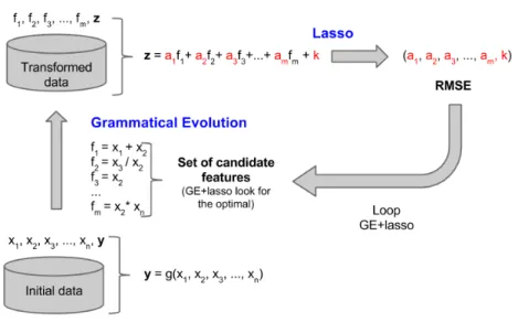
Figure 2 shows the proposed methodology approach for the optimization of system modeling problem. De-tailed explanations of the different phases are summa-rized in the following subsections.
4.1 GE feature selection
Given an extensive set of parameters that may cause an effect on system performance, FE selects the optimal set that best describes the system behavior. Also, this tech-nique, which is provided by GE, avoids the inclusion of irrelevant features while incorporating correlations and combinations of representative variables.
The input to our approach consists of a vector of initial data that includes the entire set of variablesxn extracted from the system.
y=g1(x1, x2, x3, . . . , xn) (2)
All these parameters are entered in the GE algorithm to start the optimization process.
Fig. 2 Optimized modeling using GE+lassomethodology.
Each individual of the GE encodes its own set of candidate featuresf1, f2, f3, . . . , fm. The candidate
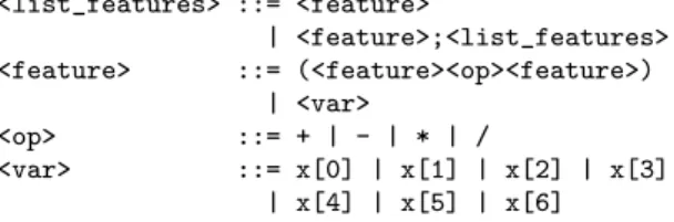
fea-tures follow the rules imposed by a BNF grammar al-lowing the occurrence of a wide variety of operations and operands to favor building optimal sets of features. Figure 3 shows an example of a BNF grammar for this approach. <list_features> ::= <feature> | <feature>;<list_features> <feature> ::= (<feature><op><feature>) | <preop>(<feature>) | <var> <op> ::= + | - | * | / <preop> ::= exp | sin | cos | ln <var> ::= x[0] | x[1] | x[2] | x[3]
| x[4] | x[5] | ... | x[n]
Fig. 3 Grammar in BNF format.xvariables, withi= 0. . . n, represent each parameter obtained from the system.
This grammar provides the operations +, −, ∗, / and preoperators exp, sin, cos, ln. The space of solu-tions is easily modified by incorporating a broader set of relationships between operands to the BNF grammar.
The output of the GE stage consists of a matrix that includes all the candidate features provided by individ-uals. Each individual output vector has its own set ofm candidate features that intends to minimize the fitness function provided for the system optimization.
z=g2(f1, f2, f3, . . . , fm) (3)
4.2Lasso generic model generation
Modeling procedures usually intend to interpret sys-tems’ behavior. They have the purpose of acquiring additional knowledge from the final models once these have been derived. Linearity, convexity and differentia-bility offered bylasso classic regression helps modeling to be a more explanatory and repeatable process. In addition, whereas GE is able to find complex symbolic expressions, GE does not perform well in parameter identification, mainly because the exploration of real numbers is not easily representable in BNFs. Due to these facts, we have included lasso algorithm in our methodology in order to manage the coefficient gener-ation of the system model.
As can be seen in Figure 2, each individual of the GE provides a set of candidate features tolasso. This clas-sical regression is in charge of deriving the optimized model for each individual by solving the following equa-tion.
z=a1f1+a2f2+a3f3+· · ·+amfm+k (4)
Lasso offers the set of optimized coefficients (a1,a2,
a3, . . ., am, k) for each individual that minimizes the fitness function. This process provides the goodness of each individual. All this information feeds back the GE algorithm to generate the next population of individu-als through selection, crossover and mutation, creating a loop. The loop continues executing until it completes the number of generations defined by the GE. This pro-cess results in the set of models that best fits system performance.
4.3 Fitness evaluation
As our main target is to build accurate models, our fitness function includes the error resulting in the es-timation process. The fitness function presented in 5 leads the evolution to obtain optimized solutions thus minimizing Root Mean Square Error or RMSD.
F = s 1 N · X n en2 (5) en=|P(n)−Pb(n)|, 1≤n≤N (6)
Estimation errorenrepresents the deviation between
the measure given by system monitoringP, and the es-timation obtained by the model Pb. n represents each
sample of the entire set ofN samples used to train the algorithms.
5 Case Study
In this section we describe a particular case study for the application of the devised methodology presented in Section 4. The problem to be solved is the fast and accu-rate estimation of the power consumption in virtualized enterprise servers performing Cloud applications. Our power model considers heterogeneity of servers, as well as specific technological features and non-traditional parameters of the target architecture that affect power consumption. Hence, we propose our modeling tech-nique that considers all these factors by combining the benefits of both GE algorithms and classical lasso re-gressions.
Firstly, a GE algorithm is applied to extract those relevant features that best describe power consump-tion sources. Features may also include correlaconsump-tions and combinations of representative variables due to FE per-formed by GE. Then, thelasso algorithm takes the op-timal set of features in order to infer an expression that characterizes the power behavior of the target architec-ture of a Cloud server. As a result, we derive a highly accurate, linear and convex power model, targeting a specific server architecture, that is automatically gen-erated by our evolutionary methodology.
We apply our methodology described in Section 4 to real measures gathered from a high-end Cloud server in order to infer an accurate power model. Also, we provide an experimental scenario for various workloads with the purpose of building and testing our methodol-ogy.
5.1 Data compilation
Data have been collected gathering real measures from a Fujitsu RX300 S6 server based on an Intel Xeon E5620 processor. This high-end server has a RAM memory of 16GB and is running a 64bit CentOS 6.4 OS virtualized by the QEMU-KVM hypervisor. Physical resources are assigned to four KVM virtual machines, each one with a CPU core and a 4GB RAM block.
The power consumption of a high-end server usually depends on several factors that affect both dynamic and static behavior [2]. Our proposed case study takes into account the following 7 variables:
– Ucpu: CPU utilization (%) – Tcpu: CPU temperature (Kelvin) – Fcpu: CPU frequency (GHz) – Vcpu: CPU voltage (V)
– Umem: Main memory utilization (Memory accesses per cycle)
– Tmem: Main memory temperature (Kelvin) – Fan: Fan speed (RPM)
Power consumption is measured with a current clamp with the aim of validating our approach. CPU and main memory utilization are monitored using hardware coun-ters collected withperf monitoring tool. On board sen-sors are checked via IPMI to get both CPU and mem-ory temperatures and fan speed. CPU frequency and voltage are monitored viacpufreq-utils Linux package. To build a model that includes power dependance with these variables, we use this software tool to modify CPU DVFS modes during workload execution. Also room temperature has been modified in run-time with the goal of finding non-traditional consumption sources that are influenced by this variable.
5.2 Experimental workload
We define three workload profiles (i) synthetic, (ii) Cloud and (iii) HPC over Cloud as they emulate different uti-lization patterns that could be found in typical Cloud infrastructures.
5.2.1 Synthetic benchmarks
The use of synthetic load allows to specifically stress different server resources. The importance of using syn-thetic load is to include situations that do not meet the actual real workloads that we have selected. Thus, the range of possible values of the different variables is ex-tended in order to adapt the model to fit future work-load characteristics and profiles.Lookbusy1stresses
ferent CPU hardware threads to a certain utilization avoiding memory or disk usage. The memory subsys-tem is also stressed separately using a modified version ofRandMem2. We have developed a program based on this benchmark to access random memory regions in-dividually, with the aim of exploring memory perfor-mance. Lookbusy and RandMem have been executed, in a separated and combined fashion, onto 4 parallel Virtual Machines that consume entirely the available computing resources of the server.
On the other hand, real workload of a Cloud data center is represented by the execution of Web Search, from CloudSuite3, as well as by SPEC CPU2006 mcf
andSPEC CPU2006 perlbench [19].
5.2.2 Cloud workload
Web Searchcharacterizes web search engines, which are typical Cloud applications. This benchmark processes client requests by indexing data collected from online sources. Our Web Search benchmark is composed of three VMs performing as index serving nodes (ISNs) of Nutch 1.2. Data are collected in the distributed file system with a data segment of 6 MB, and an index of 2 MB that is crawled from the public Internet. One of this ISNs also executes a Tomcat 7.0.23 frontend in charge of sending index search requests to all the ISNs. The fron-tend also collects ISNs responses and sends them back to the requesting client. Client behavior is generated by Faban 0.7 performing in a fourth VM. Resource uti-lization depends proportionally on the number of clients accessingWeb Search. Our number of clients configura-tion ranges from 100 to 300 to expose more informaconfigura-tion about the application performance. The four VMs use all the memory and CPU resources available in each server.
5.2.3 HPC over Cloud
In order to represent HPC over a Cloud computing in-frastructure, we chooseSPEC CPU2006 mcf and perl-benchas they are memory and intensive, and CPU-intensive applications, respectively.SPEC CPU2006 mcf consists on a network simplex algorithm accelerated with a column generation that solves large-scale minimum-cost flow problems. On the other hand, a mail-based benchmark is performed bySPEC CPU2006 perlbench. This program applies a spam checking software to ran-domly generated email messages. Both SPEC applica-tions are run in parallel in 4 VMs using entirely the available resources of the server.
2 http://www.roylongbottom.org.uk 3 http://parsa.epfl.ch/cloudsuite
Instead of restricting the use of synthetic workloads only for training the algorithms, and limiting the use of real Cloud benchmarks exclusively for testing, we have used both workloads for the two purposes. This procedure provides automation for the progressive in-corporation of additional benchmarks to the model.
For each run of the combined GE+lasso approach, we randomly select 50% of each data set (synthetic, Web Search, SPEC CPU2006 mcf and perlbench) for training and the remaining 50% for testing stage. This technique validates the variability and versatility of the system, by analyzing the occurrence of local minima in optimization scenarios.
6 Experimental results
As we stated in section 5, tests have been conducted gathering real data from our Fujitsu server. Our exper-iments present high variability for the different features compiled from the server.
– CPU operation frequency (Fcpu) is fixed to f1 =
1.73 GHz, f2 = 1.86 GHz, f3 = 2.13 GHz, f4 =
2.26 GHz, f5 = 2.39 GHz and f6 = 2.40 GHz;
thus modifying CPU voltage (Vcpu) from 1.73 V to 2.4 V.
– Room temperature has been modified in run-time, from 17◦C to 27◦C. Therefore, temperatures of CPU and memory (Tcpu and Tmem) range from 306 K to 337 K, and from 298 K to 318 K respectively. – CPU and memory utilizations (Ucpu and Umem)
take values from 0% to 100% and from 0 to 0.508 memory accesses (cache-misses) per CPU cycle re-spectively.
– Finally, due to both room temperature, and CPU and memory utilization variations, fan speed values (Fan) range from 3540 RPM to 7200 RPM.
Data have been split into training and testing sets. Training stage performs feature selection and builds the power model according to our grammar and fitness function. Next, the testing stage examines the power model accuracy. The algorithm proposed by our method-ology is executed completely 20 rounds using the same grammar and fitness function configuration. For each run, we randomly select 50% of each data set for train-ing and 50% for testtrain-ing stage, thus obtaintrain-ing 20 final power models. This procedure validates the variability and versatility of the system, by analyzing the occur-rence of local minima in optimization scenarios.
6.1 Algorithm setup
6.1.1 GE setup parameters
We use GE to obtain a set of candidate features that best describe our optimization problem. To obtain ade-quate solutions we tune the algorithm using the follow-ing parameters:
– Population size: 250 individuals – Number of generations: 3000 – Chromosome length: 100 codons
– Mutation probability: inversely proportional to the number of rules, 1/4 in our case.
– Crossover probability: 0.9 – Maximum wraps: 3 – Codon size: 256
– Tournament size: 2 (binary)
As we strictly seek for simple combination of fea-tures, our proposed BNF grammar only provides the operations +| − | ∗ |/. The space of solutions is easily increased by incorporating more complex relationships between operands to the BNF grammar. Figure 4 shows the BNF grammar proposed for this case study.
<list_features> ::= <feature> | <feature>;<list_features> <feature> ::= (<feature><op><feature>) | <var> <op> ::= + | - | * | / <var> ::= x[0] | x[1] | x[2] | x[3] | x[4] | x[5] | x[6]
Fig. 4 Grammar in BNF format.xvariables, withi= 0. . .6, represent processor and memory temperatures, fan speed, processor and memory utilization percentages, processor fre-quency and voltage, respectively.
6.1.2 Lasso setup parameters
We use thelassoalgorithm to obtain a set of candidate solutions with low error, when compared with the real power consumption measures in order to solve our op-timization modeling problem. Lasso setup parameters are the following:
– Number of observations: 100
– λregularization parameter: Geometric sequence of 100 values, the largest just sufficient to produce zero coefficients.
– λregularization parameter: 1·10−4
6.2 Training stage
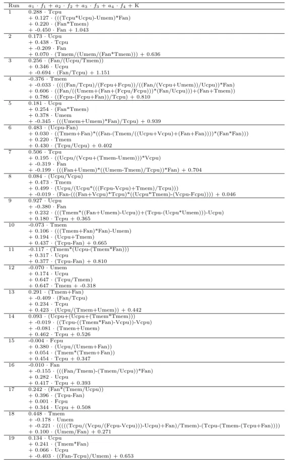
We have performed variable standardization for every feature (in the range [1,2]) to assure the same prob-ability of appearance for all the variables and to en-hance the GE symbolic regression. Experiments with more than 4 features do not provide better values for RMSD. Hence, we have bounded their occurrence to a maximum of 4 by penalizing higher number of fea-tures in our fitness evaluation function. This also facili-tates the generation of simpler models, which are faster and easy to be applied, in order to be used for real-time power optimizations. Table 1 shows phenotypes of each feature combined with the coefficients provided bylassothat are obtained for 20 complete executions of our methodology algorithm. Fitness results, that corre-spond to the RMSD between measured and estimated power consumption (see Equation 5), are shown in Ta-ble 2 for the training stage. Both TaTa-ble 1 and TaTa-ble 2 present the results for the best model of each execution. As can be seen in Table 1, power model solutions combine features that correspond to a single variable with others that merge a combination of several param-eters. On the one hand, there are single variable features that appear in up to 50% of the power model solutions. This shows that there are linear dependencies with cer-tain parameters, as Ucpu, Tpcu, and Tmem that are consistent regardless of the workload that is used for training and testing. On the other hand, variables as Vcpu,Fcpu andUmem are seldom treated as a feature in the model solutions. However, they systematically appear when combined with other variables. These re-sults show how there exist input parameters that are not relevant for the modeling or they are correlated to other features, and their inclusion could decrease the model accuracy. Model training for run 10 shows the lowest RMSD error of 0.1067.
6.3 Model testing
At this stage, we analyze the quality of the models that we have simultaneously tested for the 20 complete exe-cutions of our methodology algorithm. Results are also analyzed particularly for the testing data that corre-sponds to each benchmark dataset in order to verify the estimation reliability of the models for different work-loads. Table 2 shows testing average error percentages particularized for the different benchmark data sets. These values have been obtained according to the fol-lowing formulation: eAVG= v u u t 1 N · X n (|P(n)−Pb(n)| ·100 P(n) ) 2 ,1≤n≤N(7)
Table 1 Power models obtained by combining GE features andlassocoefficients for 20 executions Run a1·f1+a2·f2+a3·f3+a4·f4+ K 1 0.288·Tcpu + 0.127·(((Tcpu*Ucpu)-Umem)*Fan) + 0.220·(Fan*Tmem) + -0.450·Fan + 1.043 2 0.173·Ucpu + 0.438·Tcpu + -0.209·Fan + 0.070·(Tmem/(Umem/(Fan*Tmem))) + 0.636 3 0.256·(Fan/(Ucpu/Tmem)) + 0.346·Ucpu + -0.694·(Fan/Tcpu) + 1.151 4 -0.376·Tmem + -0.033·((((Fan/Tcpu)/(Fcpu+Fcpu))/((Fan/(Vcpu+Umem))/Ucpu))*Fan) + 0.606·((Fan/((Umem+(Fan+(Fcpu/Fcpu)))*(Fan/Ucpu)))+(Fan+Tmem)) + 0.786·((Fcpu-(Fcpu+Fan))/Tcpu) + 0.810 5 0.181·Ucpu + 0.254·(Fan*Tmem) + 0.378·Umem + -0.345·(((Umem+Umem)*Fan)/Tcpu) + 0.939 6 0.483·(Ucpu-Fan) + 0.030·((Tmem+Fan)*((Fan-(Tmem/((Ucpu+Vcpu)+(Fan+Fan))))*(Fan*Fan))) + 0.220·Tmem + 0.430·(Tcpu/Ucpu) + 0.402 7 0.506·Tcpu + 0.195·((Ucpu/(Vcpu+(Tmem-Umem)))*Vcpu) + -0.319·Fan + -0.199·(((Fan+Umem)*((Umem-Tmem)/Tcpu))*Fan) + 0.704 8 0.084·(Ucpu/Vcpu) + 0.473·Tmem + 0.499·(Ucpu/(Ucpu*(((Fcpu-Vcpu)+Tmem)/Tcpu))) + -0.019·(Fan-(((Fan+Vcpu)*Tcpu)*((Ucpu*Tmem)-(Vcpu-Fcpu)))) + 0.046 9 0.927·Ucpu + -0.380·Fan + 0.232·(((Tmem*((Fan+Umem)-Ucpu))+(Tcpu-(Ucpu*Umem)))-Ucpu) + 0.180·Tcpu + 0.365 10 -0.073·Tmem + 0.106·(((Tmem+Fan)*Fan)-Umem) + 0.194·(Ucpu+Tmem) + 0.437·(Tcpu-Fan) + 0.665 11 -0.117·(Tmem*(Ucpu-(Tmem*Fan))) + 0.317·Ucpu + 0.377·(Tcpu-Fan) + 0.810 12 -0.070·Umem + 0.174·Ucpu + 0.647·(Tcpu/Tmem) + 0.647·Tmem + -0.318 13 0.291·(Tmem+Fan) + -0.409·(Fan/Tcpu) + 0.234·Tcpu + 0.423·(Ucpu/(Tmem+Umem)) + 0.442 14 0.093·(Ucpu+(Ucpu+(Tmem*Tmem))) + -0.019·((Tcpu-((Tmem*Fan)-Vcpu))-Vcpu) + -0.081·(Tmem+Umem) + 0.462·Tcpu + 0.526 15 -0.004·Fcpu + 0.380·(Ucpu/(Umem+Fan)) + 0.054·(Tmem*(Tmem+Fan)) + 0.454·Tcpu + 0.347 16 -0.010·Fan + -0.155·(((Fan/Tmem)-(Tmem/Ucpu))*Fan) + 0.282·Ucpu + 0.417·Tcpu + 0.393 17 0.242·(Fan*(Tmem/Ucpu)) + 0.396·(Tcpu-Fan) + 0.001·Fcpu + 0.344·Ucpu + 0.508 18 0.448·Tmem + -0.178·Umem + -0.221·(((((Tcpu/(Vcpu/(Fcpu-Vcpu)))-Ucpu)+Fan)/Tmem)-(Tcpu-(Tmem-(Tcpu+Fan)))) + 0.100·(Umem/Fan) + 0.271 19 0.134·Ucpu + 0.241·(Tmem*Fan) + 0.066·Ucpu + -0.403·((Fan-Tcpu)/Umem) + 0.653 20 -0.433·(((Fan-(Ucpu+Umem))/Fan)-(Tcpu+Fan)) + -0.295·Umem + -0.102·Fan + 0.235·(((Tmem-Umem)-Ucpu)+Fan) + 0.184
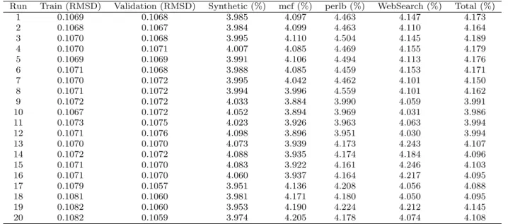
Table 2 RMSD and Average testing error percentages for 20 executions
Run Train (RMSD) Validation (RMSD) Synthetic (%) mcf (%) perlb (%) WebSearch (%) Total (%)
1 0.1069 0.1068 3.985 4.097 4.463 4.147 4.173 2 0.1068 0.1067 3.984 4.099 4.463 4.110 4.164 3 0.1070 0.1068 3.995 4.110 4.504 4.145 4.189 4 0.1070 0.1071 4.007 4.085 4.469 4.155 4.179 5 0.1069 0.1069 3.991 4.106 4.494 4.113 4.176 6 0.1071 0.1068 3.988 4.085 4.459 4.153 4.171 7 0.1070 0.1072 3.995 4.042 4.462 4.101 4.150 8 0.1071 0.1072 3.994 3.996 4.559 4.101 4.162 9 0.1072 0.1072 4.033 3.884 3.990 4.059 3.991 10 0.1067 0.1072 4.052 3.894 3.969 4.031 3.986 11 0.1073 0.1075 4.023 3.926 3.963 4.063 3.994 12 0.1071 0.1076 4.098 3.896 3.951 4.030 3.994 13 0.1070 0.1070 4.073 3.939 4.173 4.243 4.107 14 0.1072 0.1072 4.088 3.935 4.174 4.184 4.096 15 0.1071 0.1070 4.083 3.922 4.161 4.246 4.103 16 0.1071 0.1070 4.060 3.937 4.164 4.217 4.095 17 0.1079 0.1057 3.951 4.136 4.208 4.056 4.088 18 0.1081 0.1060 3.981 4.171 4.180 4.050 4.095 19 0.1082 0.1060 3.953 4.190 4.224 4.212 4.145 20 0.1082 0.1059 3.974 4.205 4.178 4.074 4.108
where P is the power measure given by the current clamp andPb is the power estimated by the model
phe-notype.nrepresents each sample of the entire set ofN samples.
Total average error for the testing dataset shows lowest error of 3.98% (as shown in Table 2). Best test-ing error corresponds to the solution with lower traintest-ing error. Solutions can be broken down for those samples that belong to different tests, achieving testing errors of 4.052%, 3.894%, 3.969% and 4.031% for synthetic, SPEC CPU2006 mcf, SPEC CPU2006 perlbench and WebSearch workloads respectively. This fact confirms that our methodology works well for our scenario, ex-tracting optimized sets of features and coefficients that are consistent even for 20 runs with random selection of both training and testing dataset.
Our methodology application shows very accurate testing results for all of the whole executions ranging from 3.98% to 4.18%. The obtained results are robust, as they have been obtained for a heterogeneous mix of workloads so the power models are not workload-dependant. According to these results, we can infer that our methodology is effective for performing fea-ture selection and building accurate multi-parametric, linear, convex and differentiable power models for high-end Cloud servers. This technique can be considered as a starting point for implementing energy optimization policies for Cloud computing facilities.
7 Conclusions
This paper has presented a novel work in the field of FE and SR for the automatic inference of accurate models.
Resulting models include combination and correlation of variables due to the FE and SR performed by GE. Therefore, the models incorporate the optimal selection of representative features that best describe the target problem while providing linearity, convexity and differ-entiability characteristics.
As a proof of concept, the devised methodology has been applied to a current computing problem, the power modeling of high-end servers in a Cloud environment. In this context, the proposed methodology has shown relevant benefits with respect to state-of-the-art ap-proaches, like better accuracy and the opportunity to consider a broader number of input parameters that can be exploited by further power optimization techniques.
8 Acknowledgments
Research by Marina Zapater has been partly supported by a PICATA predoctoral fellowship of the Moncloa Campus of International Excellence (UCM-UPM). This work has been partially supported by the Spanish Min-istry of Economy and Competitiveness, under contracts TIN2008-00508, TEC2012-33892 and IPT-2012-1041-430000, and INCOTEC. The authors thankfully ac-knowledge the computer resources, technical expertise and assistance provided by the Centro de Supercom-putaci´on y Visualizaci´on de Madrid (CeSViMa).
References
1. Adiga, N., et al: An Overview of the BlueGene/L Super-computer. In: Supercomputing, ACM/IEEE 2002 Con-ference, pp. 60–60 (2002)
2. Arroba, P., Risco-Mart´ın, J.L., Zapater, M., Moya, J.M., Ayala, J.L., Olcoz, K.: Server power modeling for run-time energy optimization of cloud computing facilities. In: Proceedings of the 5th International Conference in Sustainability in Energy and Buildings (SEB´14) (2014). (Accepted, to appear in 2014)
3. Back, T., Hammel, U., Schwefel, H.P.: Evolutionary com-putation: comments on the history and current state. Evolutionary Computation, IEEE Transactions on1(1), 3–17 (1997). DOI 10.1109/4235.585888
4. Bar-Yam, Y.: Dynamics of Complex Systems. Addison-Wesley stydies in nonlinearity. Westview Press (1997) 5. Berl, A., Gelenbe, E., Di Girolamo, M., Giuliani, G.,
De Meer, H., Dang, M.Q., Pentikousis, K.: Energy-efficient cloud computing. Comput. J.53(7), 1045–1051 (2010)
6. Bianchi, L., Dorigo, M., Gambardella, L.M., Gutjahr, W.J.: A survey on metaheuristics for stochastic com-binatorial optimization. Natural Computing: An inter-national journal 8(2), 239–287 (2009). DOI 10.1007/ s11047-008-9098-4
7. Blum, C., Roli, A.: Metaheuristics in combinatorial opti-mization: Overview and conceptual comparison. ACM Comput. Surv. 35(3), 268–308 (2003). DOI 10.1145/ 937503.937505
8. Boccara, N.: Modeling Complex Systems. Graduate Texts in Physics. Springer (2010)
9. Bohra, A., Chaudhary, V.: Vmeter: Power modelling for virtualized clouds. In: IPDPSW, pp. 1–8 (2010) 10. Brandon, J.: Going green in the data center:
Practi-cal steps for your sme to become more environmentally friendly. Processor29(39), 1–30 (2007)
11. Buyya, R., et al.: Energy-efficient management of data center resources for cloud computing: A vision, architec-tural elements, and open challenges. In: PDPTA 2010. Las Vegas, USA (2010)
12. Chen, Q., et al.: Profiling energy consumption of vms for green cloud computing. In: DASC, pp. 768–775 (2011) 13. Contreras, G., Martonosi, M.: Power prediction for
in-tel xscale processors using performance monitoring unit events. In: ISLPED, pp. 221–226. New York, NY, USA (2005)
14. El-Sayed, N., Stefanovici, I.A., Amvrosiadis, G., Hwang, A.A., Schroeder, B.: Temperature management in data centers: why some (might) like it hot. SIGMETRICS Perform. Eval. Rev.40(1), 163–174 (2012)
15. Ge, R., et al.: Performance-constrained distributed dvs scheduling for scientific applications on power-aware clus-ters. In: Supercomputing Conference, SC ’05, pp. 34–34. IEEE Computer Society, Washington, DC, USA (2005) 16. Goldberg, D.E.: Genetic Algorithms in Search,
Optimiza-tion, and Machine Learning. Addison-Wesley Profes-sional (1989)
17. Google Data Centers: Efficiency: How we do it. Temperature control. http://www.google.com/intl/ en_ALL/about/datacenters/efficiency/internal/ #temperature(2014)
18. Hemberg, E., Ho, L., O’Neill, M., Claussen, H.: A com-parison of grammatical genetic programming grammars for controlling femtocell network coverage. Genetic Pro-gramming and Evolvable Machines14(1), 65–93 (2013). DOI 10.1007/s10710-012-9171-8
19. Henning, J.L.: Spec cpu2006 benchmark descriptions. SIGARCH Comput. Archit. News 34(4), 1–17 (2006). DOI 10.1145/1186736.1186737
20. Hsu, C.H., Feng, W.C.: A power-aware run-time system for high-performance computing. In: Supercomputing Conference, pp. 1–1 (2005)
21. Kaplan, J., Forrest, W., Kindler, N.: Revolutionizing data center energy efficiency. Tech. Rep. July, McKinsey & Company (2008)
22. Lewis, A., et al.: Run-time energy consumption estima-tion based on workload in server systems. In: HotPower, pp. 4–4. Berkeley, CA, USA (2008)
23. Markoff, J., Lohr, S.: Intel’s huge bet turns iffy. New York Times Technology Section (2002)
24. Meisner, D., et al.: Peak power modeling for data center servers with switched-mode power supplies. In: ISLPED, pp. 319–324. New York, NY, USA (2010)
25. Miller, R.: Google: Raise your data center temperature. http://www.datacenterknowledge.com/archives/2008/ 10/14/google-raise-your-data-center-temperature/ (2008)
26. O’Neill, M., Ryan, C.: Grammatical evolution. Evolu-tionary Computation, IEEE Transactions on5(4), 349– 358 (2001). DOI 10.1109/4235.942529
27. P. Niles and P. Donovan: Virtualization and Cloud Com-puting: Optimized Power, Cooling, and Management Maximizes Benefits. White paper 118. Revision 3. Tech. rep., Schneider Electric (2011)
28. Pelley, S., et al.: Understanding and abstracting total data center power. In: WEED (2009)
29. Ryan, C., Collins, J., Neill, M.: Grammatical evolu-tion: Evolving programs for an arbitrary language. In: W. Banzhaf, R. Poli, M. Schoenauer, T. Fogarty (eds.) Genetic Programming,Lecture Notes in Computer Sci-ence, vol. 1391, pp. 83–96. Springer Berlin Heidelberg (1998). DOI 10.1007/BFb0055930
30. Scheihing, P.: Creating energy efficient data center. In: Data Center Facilities and Engineering Conference. Washington DC, USA (2007)
31. Tibshirani, R.: Regression shrinkage and selection via the lasso. Journal of the Royal Statistical Society. Series B (Methodological)58(1), pp. 267–288 (1996)
32. Turner, C.R., Fuggetta, A., Lavazza, L., Wolf, A.L.: A conceptual basis for feature engineering. Journal of Systems and Software 49(1), 3 – 15 (1999). DOI 10.1016/S0164-1212(99)00062-X
33. Vladislavleva, E., Smits, G., den Hertog, D.: Order of nonlinearity as a complexity measure for models gener-ated by symbolic regression via pareto genetic program-ming. Evolutionary Computation, IEEE Transactions on 13(2), 333–349 (2009). DOI 10.1109/TEVC.2008.926486 34. Warkozek, G., et al.: A new approach to model energy consumption of servers in data centers. In: ICIT, pp. 211–216 (2012)
35. Warren, M., et al.: High-density computing: A 240-processor beowulf in one cubic meter. In: Supercomput-ing Conference, pp. 61–61 (2002)