This is the author manuscript accepted for publication and has undergone full
Revising Commitments: Field Evidence on the Adjustment of
Prior Choices
Xavier Giné, Jessica Goldberg, Dan Silverman, and Dean Yang*
Abstract
We implement an artefactual field experiment in rural Malawi to study revisions of prior choices regarding future income receipts. This allows examination of intertemporal choice revision and its determinants. New tests provide evidence of self-control problems for some participants. Revisions of money allocations toward the present are positively associated with refined measures of present-bias from an earlier survey, and with the randomly assigned closeness in time to the first possible date of money disbursement. We find little evidence that revisions of allocations toward the present are associated with spousal preferences for such revision, household shocks, or the financial sophistication of respondents.
*
Giné: Development Economics Research Group, World Bank and BREAD
([email protected]); Goldberg: Department of Economics, University of Maryland
([email protected]); Silverman: Department of Economics, Arizona State University and NBER ([email protected]); Yang: Ford School and Department of Economics, University of Michigan, NBER, and BREAD ([email protected]). Niall Keleher, of Innovations for Poverty Action, was instrumental to the design and implementation of this study. We thank him for his important contributions to this project. We also thank James Andreoni, Stefano DellaVigna, Pascaline Dupas, Yoram Halevy, Vivian Hoffmann, Glenn Harrison, Pam Jakiela, Damon Jones, David I. Levine, Stephan Meier, Ted Miguel, Matthew Rabin, and participants in several seminars for their many helpful comments. We thank Lasse Brune, Jason Kerwin, and Prachi Jain for excellent research assistance. Data and codes that replicate the results are available in the Economic Journal website.
Keywords: commitment, hyperbolic preferences, lab experiment, consumption
smoothing, self-control, Malawi
JEL codes: D81, D91, O10
Revising Commitments: Field Evidence on the Adjustment of
Prior Choices
Xavier Giné, Jessica Goldberg, Dan Silverman, and Dean Yang*
Abstract
We implement an artefactual field experiment in rural Malawi to study revisions of prior choices regarding future income receipts. This allows examination of intertemporal choice revision and its determinants. New tests provide evidence of self-control problems for some participants. Revisions of money allocations toward the present are positively associated with refined measures of present-bias from an earlier survey, and with the randomly assigned closeness in time to the first possible date of money disbursement. We find little evidence that revisions of allocations toward the present are associated with spousal preferences for such revision, household shocks, or the financial sophistication of respondents.
Keywords: commitment, hyperbolic preferences, lab experiment, consumption
smoothing, self-control, Malawi
JEL codes: D81, D91, O10
* Giné: Development Economics Research Group, World Bank and BREAD
([email protected]); Goldberg: Department of Economics, University of Maryland
([email protected]); Silverman: Department of Economics, Arizona State University and NBER ([email protected]); Yang: Ford School and Department of Economics, University of Michigan, NBER, and BREAD ([email protected]). Niall Keleher, of Innovations for Poverty Action, was instrumental to the design and implementation of this study. We thank him for his important contributions to this project. We also thank James Andreoni, Stefano DellaVigna, Pascaline Dupas, Yoram Halevy, Vivian Hoffmann, Glenn Harrison, Pam Jakiela, Damon Jones, David I. Levine, Stephan Meier, Ted Miguel, Matthew Rabin, and participants in several seminars for their many helpful comments. We thank Lasse Brune, Jason Kerwin, and Prachi Jain for excellent research assistance. Data and codes that replicate the results are available in the Economic Journal website.
The well-being of individuals, especially those who live close to subsistence, depends importantly on the ability to make and execute intertemporal plans. The world over, however, individuals close to subsistence appear to leave con-sumption unsmooth, save at a low rate, or fail to use inexpensive agricultural and health inputs.
While these observed choices may be optimal given the constraints that individuals face and the incompleteness of markets, researchers have suggested that they may be the result of self-control problems.1
In this paper, we investigate several potential sources of failure to pursue intertemporal plans by studying why choices about future consumption are revised. The paper makes two contributions. First, we test for the presence of self-control problems using a novel and robust method. Second, we provide a quantitative analysis of this and other motives for the adjustment of prior choices.
Applied research typically models self-control problems as the result of present-biased (quasi-hyperbolic) time discounting. This modelling strategy is founded, in part, on evidence of non-constant time discounting. Several studies can be interpreted to show that time discount rates decline as tradeoffs are pushed into the temporal distance.2
In particular, many experimental studies document “static” preference reversals: subjects choose the larger and later of two rewards when both are distant in time, but prefer the smaller and earlier one as both rewards draw nearer to the present.
Interpreted as present-biased time discounting and assuming time-separable preferences, these static preference reversals imply time-inconsistency: the choices (plans) that a person makes now about consumption at a later date are different from the choices she would make when that date arrives.3
Self-1
Some of the seemingly puzzling evidence regarding intertemporal choices of the poor were first summarised by Theordore Schultz in his 1979 Nobel Prize lecture and more re-cently in Banerjee and Duflo (2011).
2Ainslie (1992), Thaler (1991) and Loewenstein and Elster (1992) provide reviews. 3Early contributions include Phelps and Pollak (1968), Laibson (1997) and O’Donoghue and Rabin (1999). See DellaVigna (2009) and Bryan, Karlan and Nelson (2010) for recent
control problems and a demand for commitment may thus emerge.4
However, until recently there have been no studies in the literature of whether static preference reversals are associated with time-inconsistency. To our knowledge, Halevy (2015) is the sole experiment in which the revision of previous decisions is a variable of interest. Augenblick et al. (2015) study revision of prior choices, focusing on dynamic inconsistency in monetary ver-sus real effort choices. Otherwise, existing work has either studied the static preference reversals themselves, the stability of time preferences, or the rela-tionship between static preference reversals and the demand for commitment. While demand for commitment is, like time-inconsistency, a signature pre-diction of (quasi-)hyperbolic discounting models, studies that focus on the demand for commitment may understate self-control problems either because commitment devices are poorly designed and thus not demanded (Beshears et al., 2011) or because demand for commitment requires some sophistication on the part of respondents: individuals who are na¨ıve about their self-control problems should not want to limit their future choices.
Testing the central mechanism linking static preference reversals to self-control problems – by investigating the correlation between them and the re-vision of prior choices – is important because the static reversals can be driven by different factors.5
For example, static preference reversals may reflect pre-dictable changes in the marginal utility of consumption.6
Alternatively, static preference reversals may reflect inattention, confusion about tradeoffs, or re-sponses to perceived experimenter demands.7
Finally, even if preferences
un-reviews of empirical applications.
4Ashraf et al (2006), Duflo et al (2011), Dupas and Robinson (2011), Brune et al (2016). 5Halevy (2015) distinguishes between time-consistency, time-invariance, and stationarity, making clear that static preference reversals are identified with non-stationarity but need not imply time-inconsistency.
6This observation has been made by Andersen et al. (2008), Andreoni and Sprenger (2012) and Ericson and Noor (2015), who note that proper inference about time discounting requires information about the curvature of the utility function.
7
Benjamin et al. (2013) document correlations among test scores, cognitive load, and short-term patience.
der commitment were well-described by changing time discount rates, simply making a plan may limit self-control problems.8
Individuals making static pref-erence reversals for any of these reasons need not exhibit time-inconsistency.
In addition, there may be other explanations for the revision of prior choices. For example, individuals from close-knit communities in developing countries are often obliged to share their income with relatives and friends, and such social pressure may prevent individuals from pursuing privately op-timal choices and the revision of previous decisions.9
Unexpected events could also motivate revisions to otherwise optimal consumption paths. Finally, in-dividuals could simply make mistakes in their original decisions, and seek to revise them later. Our analysis explores the role of these three alternative explanations.
From a policy standpoint, it is important to understand what drives revi-sion behaviour because it will influence the design of commitment devices and their welfare impact. If social pressure, shocks, or mistakes affect revisions, then commitment devices could be designed either to shield resources from one’s social network (while maintaining access for oneself), or to allow access in case of emergency or error. In contrast, if self-control problems are im-portant then commitment devices should protect resources from one’s future self.
To assess the drivers of revision behaviour, we implement an artefactual field experiment where the key dependent variable is revision of a previous decision under commitment. Our sample consists of several hundred wife-husband pairs in rural Malawi. We elicited intertemporal choices by adapting Andreoni and Sprenger’s (2012) convex time budget method, with large real
8Making plans or setting goals can affect self-control and self-efficacy (Bandura 1997, Ameriks et al. 2003). This idea is also consistent with economic models of costly self-control such as Gul and Pesendorfer (2001), Ozdendoren et al. (2012), and Fudenberg and Levine (2012), in which consumers may both seek commitment and, yet, not always exhibit time-inconsistency.
9See, e.g., Platteau (2000), Maranz (2001), Anderson and Baland (2002), Ligon et al (2002), Hoff and Sen (2006), Ashraf (2009), Baland et al (2011), Jakiela and Ozier (2011) and Schaner (2015).
stakes (roughly a month’s wages). Subjects made several choices regarding an allocation of money to be disbursed at two points, 61 and 91 days, in the future. A subset of these subjects was revisited some time prior to t = 61 and given the opportunity to revise the allocation between t= 61 and t= 91. A measure of this revision is our dependent variable. We examine correlates of this revision corresponding to each of the four potential determinants of revision outlined above.
The experiment also provides a complementary test of quasi-hyperbolic discounting models. In those models, average revisions toward sooner should be larger when the time lag between the revision decision and the first dis-bursement (t = 61) is sufficiently small. We randomised the number of days prior tot = 61 when each subject had to make the revision decision.
Analysis of initial allocations indicates that they usually, but not always adhere to the law of demand; individuals typically allocated more income to later periods when offered higher rates of return to waiting. We interpret this to indicate that most subjects understood the choices made but that some preference reversals may simply reflect confusion. We also find that “static” preference reversals are frequent, but only slightly more likely to be “present”-biased (as opposed to “future”-“present”-biased).10
Turning to revision behaviour, we find that revisions are common, often substantial in size, and shift money both sooner and later. We find some evidence that time-inconsistency induces these revisions: subjects shift more money toward sooner when: (1) their initial allocations are “present”-biased, and (2) the time lag to disbursement is shorter (when the revision decision is made six or fewer days prior to day t = 61). Importantly, the relationship between “present”-biased and revisions toward sooner is concentrated among individuals that do not exhibit anticipated changes in the marginal utility of consumption. This finding is significant because it demonstrates, in a devel-oping context, that predictable changes in the marginal utility of consumption
10
This finding contrasts other studies using the multiple price list method, but is consistent with Andreoni and Sprenger (2012).
may drive the observed static preference reversals. Put differently, we find evidence of a reason why not all “present”-biased preference reversals are the result of time-inconsistency.
We find no evidence that social pressure affects revision decisions in a mean-ingful way: respondents’ revisions are not much higher when one’s spouse’s sooner allocations are larger than one’s own, or when they have many other relatives in the village. We also find little evidence that shocks or financial sophistication (a proxy for mistakes) strongly predict revisions (although the impact is less precisely estimated).
The next section presents details of the experimental design, the sample of participants and the experimental setting. Section 2 presents the theoretical framework and derives the testable implications. Then, Section3 describes the choices under commitment and the drivers of revision behaviour. Section 4 clarifies our contribution to the related literature, and section 5 concludes.
1
The Experiment
The experiment proceeded in two stages. In stage one, we elicited intertem-poral choices under commitment. Husbands and wives each separately made several independent choices about the allocation of a substantial amount of money over time. Each choice was an allocation of an endowment between two periods, one “sooner” and one “later.” In stage two of the experiment, some households were revisited on a randomly selected day in the two weeks prior to the arrival of the first disbursement of their money in the far period and given an opportunity to revise their original far-period allocation. Surveys at both stages measured household wealth, income, and expenditures as well as the participants’ expectations for each of these variables.
1.1
The Setting
Rural Malawi has a number of advantages as a setting for experimental study of intertemporal choice. Most important, financial markets are thin especially during the rainy season when the experiment was conducted. During this lean period, study participants have virtually no cash, and borrowing is not merely expensive but it is often impossible. Similarly, short-term saving can be difficult due to limited access to banking institutions, and familial or social demands for what appears like excess cash.11
This financial market incompleteness is important because it reduces smooth-ing opportunities that confound efforts to elicit time preferences in developed economies.12
When financial markets are thick and transaction costs low, an-swers to the questions asked in typical time-preference experiments should, in theory, reflect only the market rates of return participants face, and reveal lit-tle about their preferences (Fuchs, 1982, Chabris, et al. 2008).13
Augenblick et al. (2015) address this issue by giving respondents in a US university campus choices over leisure that is hard to smooth instead of monetary prizes.
Our study location also has some disadvantages. Poor infrastructure makes the logistics of a large-scale experiment challenging. In addition, participants have low levels of formal education and may therefore find the experiment difficult to grasp. We therefore evaluate the consistency of participants’ choices with a basic prediction of standard models of economic decision-making: the law of demand. The degree of consistency with the law of demand will provide
11In Malawian survey data, only 26 percent of respondents use a formal financial product, and around 60 percent had never heard of a savings account (FinScope, 2008).
12
Grain and other consumption goods in store are used to smooth consumption, but only partially. We rely on the fact that stakes are high and that they involve cash.
13To illustrate, suppose that outside of the lab a participant can borrow or save at mar-ket rate r without transaction costs. A typical experiment asks the participant to choose between $xsooner or $ (1 +re)xlater, where re is the rate of return implied by the later
option. The participant may view this as a choice between OptionA,$xsooner and access to the interest rate r and OptionB, $ (1 +re)xlater and access to the interest rate r. If re > r, then the set of allocations under option B contains the set under option A, and
more. Thus, for any monotonic preference ordering, optionB is preferred. Analogously, if
r > rethen isApreferred.
a measure of participants’ understanding of the trade-offs involved in their decisions.
1.2
The Sample
Participants in the experiment were recruited in January and February 2010 from a population of rural households in central Malawi who were growing tobacco as their main cash crop. Participants were a subset of respondents who were participating in another simultaneous experiment on savings.14
To be eligible for inclusion in this experiment, respondents had to be located within 25 kilometers of the town of Mponela, to facilitate our cash disbursements. Due to our interest in interactions within the household, we further restricted our sample to farmers who were part of a married couple.
These sample restrictions left us with 1,268 targeted households. A total of 1,071 households (84.4%) and 2,142 respondents were successfully interviewed at baseline. A subset of 661 respondents (randomly selected from the full set of baseline respondents) make up the stage two sample to be revisited.
Table 1 provides summary statistics of baseline survey responses. In the full sample (Panel A), the median respondent is 46 years old, has 4 years of formal education, lives in a village with 177 inhabitants, including four relatives other than his or her spouse. When compared to typical households from low-income countries, the households in the sample are poor and in the central Malawi region we study, tobacco farmers have similar poverty and income levels to those of non-tobacco-producing households.15
At the time of the baseline survey, the median household in the household has a zero balance in formal bank accounts, and the 90th percentile of the bank balance distribution is
14See the Online Appendix for further details on sampling and Brune et al. (2016) for details on the broader study from which our study participants were drawn. We note that the inclusion of a dummy indicating the treatment status in the savings experiment does not change the results significantly.
15
Based on our calculations from the 2004 Malawi Integrated Household Survey (IHS), individuals in tobacco farming rural households in central Malawi live on PPP$1.48/day on average, while the average for central Malawian rural households overall is PPP$1.51/day.
just 700 Malawi Kwacha (MK), or approximately US$4.67. Including the self-reported value of assets, the median household held just 4,446 MK of wealth and the 90th percentile held 25,800 MK. Because the baseline survey was conducted during the rainy season, several months would elapse before the cash crop or primary staple (maize) would be harvested in mid-April or early May. As a result, the median household expects virtually no income between the interview date and April 2010.
1.3
Implementation of Stage One
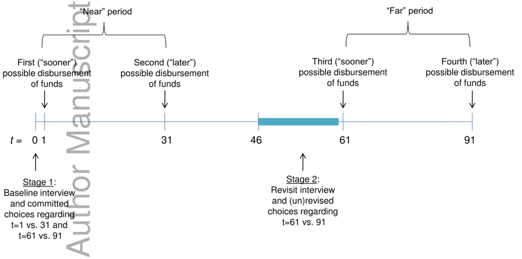
Figure 1 displays the timeline of the experiment. At the baseline interview, the household head and spouse were physically separated. After demograph-ics questions, each made 5 independent choices regarding the allocation of 2000MK between tomorrow (“sooner”) and 30 days from tomorrow (“later”). Each participant was given a bowl containing 20 beans (tokens) and two empty dishes,AandB. One token allocated to dishAcorresponded to 100M K
tomorrow. One token allocated to dish B corresponded to 100M K ∗(1 +r) 30 days from tomorrow, where r is the rate of return for waiting. The rate of return took on 5 different values: 0.10, 0.25, 0.50, 0.75, and 1.00. The rates of return rose, in order, with each of the five allocation choices, and participants knew the order before making any choices. For each rate of return, the partic-ipant made an allocation of tokens to dishes, the tokens were translated into Malawi Kwacha, and the total was written above each dish on a whiteboard. The participant was then allowed to adjust the allocation. This process was repeated until the participant was ready to make the next allocation.
After completing the first five choices, the participant answered a series of questions from the baseline survey. Then, using the same elicitation method with cup, beans, and dishes, the participant again made five independent choices regarding 2000MK, while facing different rates of return for waiting. This time, each of the five choices concerned the allocation of money between 60 and 90 days from tomorrow (the “far” time frame). Online Appendix Figure
1 presents a schematic of the allocation decision.
The interruption between the five choices in the near time frame and the five choices in the far was intentional. We sought to avoid having participants choose the same allocations in both frames simply for the sake of being (or appearing) consistent. In addition, the order in which the time preference sec-tions of the questionnaire were administered was randomly assigned between households within clubs. With probability 1
2, a participant was first presented
with the “near” time frame allocations; otherwise, the “far” allocations were presented first. Controlling for order effects does not affect the results, and the order in which time frames were presented does not predict choices.
Before making their choices, each participant was told that one member of the couple would be randomly chosen to have one of his or her choices implemented. The randomization was performed on site by rolling dice, and it was designed to favor (with two-thirds probability) the far time frame to have a large enough sample of stage two revisits. Implementation took the form of a voucher, redeemable at a disbursement office set up for this purpose in the nearest town, Mponela. The voucher indicated the allocation and was issued to the member of the couple who was randomly chosen. The recipient’s identity was established with a name and a fingerprint placed on the voucher. We made key aspects of payment delivery symmetric between the “near”and “far” time frames. In particular, we provided two vouchers, one for the “sooner” period (either the day after the visit or 60 days from then) and one for the “later” period (30 days from the day of the visit or 90 days from then, depending on time frame) redeemable for cash at the disbursement of-fice. This symmetry has advantages over a design where near payments are made in cash during the experiment. That design could favor allocations to the “sooner” period in the “near” time frame if participants mistrusted the ex-perimenters or if the infrastructure in the area induced substantial transaction costs to redeeming the “later” period voucher. A disadvantage of this symme-try is that payments were available no sooner than one day after the choices were made. Therefore, we cannot study preferences regarding consumption in
the present. To the extent that changes in time discounting are largest when tradeoffs are pushed just beyond the present, any relationships between choice under commitment and revision behaviour should be attenuated.16
1.4
Implementation of Stage Two
Stage two of the experiment was only carried out with those households whose randomly selected decision concerned an allocation in the far time frame.17
In stage two, these households were unexpectedly revisited. The target revisit date was randomly selected from the interval between 16 and 2 days prior to day 61 (the first far-frame disbursement date). Revisits occurred even if the household chose an allocation involving no disbursement of funds at day 61.18
Revisits occurred in March and April 2010.19
16This “front end delay” payment method has been used in the literature by Pender (1996), Andersen et al (2008) and Bauer et al. (2010), among others.
17Recall that in stage one of the experiment, one of each household’s 20 decisions (10 of the husband’s and 10 of the wife’s) was randomly selected to be implemented. If the selected decision concerned an allocation in the near time frame (which happened with probability one-third by design), the experimental intervention was completed for that household. The chosen individual in the household redeemed the allocation and was not interviewed again. 18In all that follows, we focus on the randomly-assigned targeted lag (in days) to first disbursement, since it is exogenous to farmer actions. We made the first attempt to revisit each respondent on the date implied by the randomly-assigned target lag. In some cases, the actual lag was shorter than the targeted lag, because some farmers could not immediately be located. The actual lag is highly correlated with the target lag; the correlation coefficient is 0.99. 84.9% of respondents were revisited with exactly the targeted lag, and 97.4% were revisited no more than two days after their target date. The maximum difference between target and actual lag is six days.
19
In stage one, participants were told, “We will give you one voucher for the money that you want sooner and one voucher for the money that you want later. Each voucher will have a date written on it, you will not be able to change these dates and will not be able to redeem the voucher before the date written on it.” Participants were not told that vouchers might be replaced or reissued. This framing, followed by the unannounced opportunity to revise the decision, may be perceived as deception. Inference in the experiment depends on respondents being unaware of the potential revision opportunity. The prohibition on deception in economic experiments derives in large part from circumstances where partic-ipants are drawn from a common pool and take part in multiple experiments (Jamison et al., 2008). The concern is that deception in one experiment will induce skepticism about
At the revisit, the wife and husband were physically separated and a survey of wealth, income, and expenditure was taken. Then, the participant whose choice had been selected to be implemented was presented with a bowl with 20 tokens. This time, four dishes were placed in front of the participant: dishes
A, B, A′
and B′
. DishesA and B contained a total of 20 tokens reflecting the participant’s original decision at baseline. DishesA′ and B′ were empty. The
participant was told that the first set of dishes showed his or her baseline choice; an allocation between what was effectively one to 16 days from the revisit and 30 days thereafter. The participant was also reminded of the rate of return for waiting that applied at baseline, and the tokens on dishes A and
B were translated into kwacha using whiteboards.
The participant was then asked to allocate the 20 tokens in the cup between the empty dishes A′
and B′
, with the same rate of return for waiting. The allocation to the second set of dishes was again translated into kwacha and the participant was asked if he or she wanted to adjust the allocation. This process was repeated until the participant indicated he or she was finished. Then a new set of vouchers were issued (regardless of whether the allocation was revised), and the interview was concluded. Appendix Figure 2 presents a schematic of the revising procedure.
Because we sought to measure revisions of prior choices, we made the original allocation decision salient and unambiguous. This procedure is also designed to balance the consequences of implicit experimenter demands. The participant must actively choose an allocation by placing tokens in the dishes, and the status quo is thus discouraged. The mere fact that we revisited the household and allowed a revision might also imply that some change is ap-propriate. However, because the original allocation is set out just next to new allocation, there should be no difficulty replicating the original allocation and perhaps some mild, implicit encouragement to do so. Given the difficulty of double blind protocols in this field setting, we cannot hope to eliminate
the experimenters’ “real´’ intent and affect behaviour in later experiments. The participants in this field experiment are not part of such common pool.
the consequences of implicit experimenter demands. Instead we designed the experiment to limit the biases they might generate.
A key element of the revisit is that participants recall the allocation they chose at baseline. The experiment therefore does not seek to study the stabil-ity of preferences after a fixed time delay (as in Harrison et al 2005). If that were the goal, we would not have reminded participants of their original choice and we would have repeated the elicitation method after a fixed delay. Our decision to make the allocation chosen at baseline salient also implies that the choice made at the revisiting stage is deterministic in a way that the baseline choices were not. The choice made at the revisiting stage will be implemented with certainty, while only one baseline choice (selected at random) was imple-mented. This difference in the choice setting may attenuate the underlying relationship between baseline choices and choices at revisiting.
The two randomizations carried out in stage one generated exogenous vari-ation in two independent variables of interest in the regression analysis. First, the implemented choice generated exogenous variation in the interest rate that applied to the revision decision. Second the targeted revisit date, generated exogenous variation in the time to first disbursement. Consistent with the fact that these two variables were randomly assigned, both the implemented interest rate and targeted days to first disbursement are for the most part uncorrelated with key baseline respondent and household characteristics. (See Section 3.1 of the Online Appendix for further details.)
2
Theoretical Framework
In this section we develop a theoretical framework to aid interpretation and the definition of measures used to analyse the revision behaviour.
We model participants’ choices in stage one as solving a problem that is simple but sufficiently flexible to allow static preference reversals both due to changing time discount rates (quasi-hyperbolic discounting) and due to
Author Manuscript
time-specific marginal utilities of consumption. We define U1(c), utility from
consumption over four periods as follows:
U1(c) = u1(c1) +β∗ 4 X τ=2 δτ−1 uτ(cτ).
The familiar “β−δ” formulation of the utility function allows static pref-erence reversals if β 6= 1. This formulation of utility also allows for a certain form of time-dependence. While utility is separable in consumption across periods, the marginal utilities of consumption may depend on time (thus the time subscriptsonus(·)). This captures the possibility that consumption has
different marginal value at different times.
Abstracting from the discrete choice set of the experiment, we can interpret the stage one decisions about the “near” time frame as solving
max
c1,c2∈R+
u1(c1) +βδu2(c2) (Near)
subject to c2 ≤(2000−c1)(1 +r)
for each rate of returnr and assuming an endowment of 2000M K. Similarly, decisions about the “far” time frame solve
max c3,c4∈R+ βδ2u3(c3) +βδ 3 u4(c4) (Far) subject to c4 ≤(2000−c3)(1 +r).
Interior solutions to these two problems satisfy the first-order conditions
u′ 1(c ∗ 1) = (1 +r)βδu ′ 2(c ∗ 2) (FOC Near) u′ 3(c ∗ 3) = (1 +r)δu ′ 4(c ∗ 4). (FOC Far)
This formulation is useful as it allows two distinct sources of static pref-erence reversals but additional assumptions on the functional form of utility
Author Manuscript
are necessary for choices to identify discount factors in problems (Near) and (Far).20
We now turn to the choices in stage two of the experiment. If the revisit is sufficiently close to period 3 then the respondent solves
max
c3,c4∈R+
Urevisit(c3, c4) = u3(c3) +βδu4(c4)
subject to c4 ≤(2000−c3)(1 +r).
Interior solutions here satisfy
u′ 3(˜c ∗ 3) = (1 +r)βδu ′ 4(˜c ∗ 4). (1)
Recall, the solution to the stage one problem (Far) satisfied
u′ 3(c ∗ 3) = (1 +r)δu ′ 4(c ∗ 4).
Thus, abstracting from uncertainty, social pressure, and mistakes, if time dis-counting is exponential (β = 1) then the respondent will not revise (˜c∗
3 =c
∗
3).
If instead the respondent is `‘present´’ -biased (β <1) then behaviour is time-inconsistent ˜c∗ 3 > c ∗ 3. Analogously, if (β >1) then ˜c ∗ 3 < c ∗ 3.
2.1
The Tests
This deterministic analysis suggests the following two tests of non-constant time discounting.
Test 1If the respondent exhibits static, “present” -biased preference reversals in stage one, and thus appears to haveβ <1, she will shift more consumption toward sooner upon revisiting. Similarly, if the respondent exhibits static,
20More formally, for any
u1, u2, βδ that can reconcile choices regarding the near term, there exists another ˜u1,u˜2,βδf that can do so as well and therefore once needs additional assumptions on the functional forms to identify β, δ and the curvature parameters of the utility function.
Author Manuscript
future-biased preference reversals in stage one and thus appears to haveβ >1,
she would shift more consumption toward later upon revisiting.
Test 2 If the revisit occurs sufficiently close to the date of first disbursement (period 3 in the above framework) then first order condition (1) applies and present (or future) bias will be evident in a revision toward sooner (later). If instead the revisit falls far before the date of first disbursement, then first order condition (FOC Far) continues to apply and the model predicts no revision.
2.1.1 Random Choice
Test 1 is appropriate if one assumes that choice data are dictated by the deterministic model above, and so the difference between the choice and the model’s prediction (or error) is interpreted as an unobserved determinant of preferences. If, however, we allow for error in the implementation of “true” preferences, estimates of the empirical model may exaggerate the correlation between static preference reversals and time-inconsistency.
To see why, consider an extreme version of that error: a respondent that makes allocations completely at random both in stage one and at the revisit. Now consider choices exhibiting “present”-bias. By definition, the allocation to sooner in the far time frame is lower than for the near time frame. When choice is entirely random, therefore, the individual will, on average, allocate more tokens to sooner upon revision. In this way, participants appearing “present”-biased due to implementation error are mechanically more likely to revise towards sooner.21
An analogous effect applies to future-biased static preference reversals and revisions toward later.
21Consider the following numerical example with interest rate
r = 10%. An individual that appears “present”-biased randomly allocates 1000 to sooner and 1100 to later in the near time frame and 600 to sooner and 1540 to later in the far time frame. Note that since the individual appears “present”-biased, the allocation to sooner in the far time frame has to be smaller than the allocation to sooner in the near time frame. In our example, the allocation to sooner is 600. But because this allocation to sooner will tend to be small, the probability that more tokens will be randomly allocated to sooner upon revisit is high, and therefore individuals that appear “present”-biased mechanically will be more likely to allocate more tokens to sooner upon revision.
We tackle this confounding effect due to implementation error in our analy-sis of Section 3 by constructing measures of “present” or future bias only from the stage one choices that were not implemented. If implementation errors are independent of each other, then measuring the tendency for static pref-erence reversals from the non-implemented choices will break the mechanical relationship between reversals and time-inconsistency in the experiment.22
2.1.2 Time-specific marginal utilities
Alternatively, while Test 1 assumes that static preference reversals are only due to non-constant time discounting, they can also emerge from time-specific marginal utilities of consumption, which may be relevant in Malawi. For example, the marginal utility of consumption may be especially high at the time of tilling or harvest (when farmers need more calories to maintain work effort) or during the period immediately prior to harvest (when caloric consumption is low).
To illustrate, suppose time discounting is constant (β = 1) but “flow” util-ity is a function of time. Suppose, in particular, that utilutil-ity is iso-elastic and varies only across, but not within, time frame:
uτ(cτ) = c1−σ τ 1−σ for τ = 1,2 and uτ(cτ) = c1−ρ τ 1−ρ for τ = 3,4 (2) σ, ρ≥0.
Interior solutions to stage one problems (FOC Near) and (FOC Far) imply
2000−c∗ 1 c∗ 1 σ = 2000−c∗ 3 c∗ 3 ρ
If optimal consumption (weakly) rises within time frame (i.e. (1 +r) ≥ δ), then respondents with a higher elasticity of intertemporal substitution in the
22See Section 4 of the Online Appendix for simulations that illustrate the consequences of using only non-implemented choices to measure a participant’s tendency to make static preference reversals.
“far” time frame will exhibit a “present”-biased static preference reversal and thus appear less patient in the “near”.23
Similarly, if the participant has a higher elasticity of intertemporal substitution within the “near” time frame (σ < ρ) then c∗
1 < c
∗
3. Such a participant would not revise his or her original
allocation (and thus would not exhibit time inconsistency) because the first order condition for the stage one problem (FOC Far) is the same as that of the revisit problem (1).
While this example relies on special functional forms, the insight is general. Differences in the curvature of flow utility across time frames can induce static preference reversals that are not driven by time inconsistency.
We accommodate this in our empirical analysis of Section 3 by identifying respondents who show differences in curvature across time frames and by al-lowing them to have a different correlation between static preference reversals and revisions of prior choices.
3
Results
We begin with an analysis of whether intertemporal choices are consistent with the law of demand and the prevalence of static preference reversals in stage one choices. We thus use all the 2,142 observations available. We then turn to stage two choices only available for the 661 individuals that were revisited.
3.1
Adherence to the Law of Demand
The additive separability and monotonicity of the flow utilities assumed in Section 2 above makes the strong prediction that if participants solve problems (Near) and (Far), then the allocation to the later period, measured in kwacha,
23
More formally, if (1 +r)≥δandσ > ρthenc∗
1> c∗3.
should increase with the rate of return to waiting r.24
We use the degree of consistency with this prediction of standard theory as a metric for judging the appropriateness of simple economic models to interpreting choices in the experiment: if choices are inconsistent with the law of demand, either poor participants did not understand the trade-offs involved, or standard economic models have little validity in this setting.
We evaluate adherence with the law of demand by dividing each partici-pant’s ten decisions into pairs, where each element of the pair is an allocation over the same two dates. The first element of the pair is the allocation to later when facing rate of return r. The other element is the allocation to later when facing the next lowest rate of return, r′
. For each participant there are eight such pairs, four for each of the two time frames. Out of 17,136 such pairs in the data, in 13,859 pairs the allocation to the later period increased with
r. Thus, 81% of pairs were consistent with the law of demand. The median violation is moderate in size in the sense that it could be made consistent with monotonicity with a reallocation of less than two tokens.25
Becker (1962) indicates that adherence with the law of demand is not a particularly stringent test of rationality because even random choice will, on average, obey the law of demand. We therefore compare the share of consistent
24To see why, think of 1
1+r as the price of consumption later in terms of consumption
sooner. Whenrgoes up, the price of later consumption goes down. The result is an income effect creating incentives to increase consumption in both periods, and a substitution effect that is positive for consumption in the later period. Thus both income and substitution effects lead to increased consumption in the later period. The near allocation, on the other hand, can go up or down depending on whether the income or substitution effect dominates. 25A comparison with existing studies in developed countries is informative as we are not aware of similar statistics being provided in studies based in developing countries. For example, in Andreoni and Sprenger (2012), the percentage of individuals that would have six or more consistent pairs of choices is 92% (using the later allocation). According to Table 2, the percentage in this experiment is somewhat lower at 76%. Similarly, using a multiple price list elicitation format Meier and Sprenger (2015) found that only 11% of a U.S. based sample exhibited multiple switch points and thus violated monotonicity – though studies of risk preferences have exhibited much higher rates of violation (e.g., Jacobsen and Petrie, 2009) than what we observe. Finally, while the published statistics are not directly comparable, the U.S. based subjects in Augenblick et al. (2015) also appear to adhere to the law of demand at higher rates than those in our study.
pairs we observe in the experiment with the share generated from a simulation where the same-sized sample makes choices purely at random (see Section 4 of the Online Appendix for details). In the simulation 57% of pairs are consistent with the law of demand.26
While substantially lower than the average rate of consistency in the experiment, this simulation suggests some caution in interpreting the choices as resulting from simple optimization and motivates disaggregated analysis.
Indeed there is important heterogeneity in consistency with the law of demand. Table 2 presents the distribution of participants by the number of times (out of eight) they increased their later allocation with a single increase in the rate of return r. Column 1 shows that, measured this way, 31.3% of participants are always consistent and 75.7% are consistent at least in 6 out of 8 allocations. At the other end of the spectrum, 10.2% of the sample violated this form of consistency in at least 4 allocations.27
In sum, these levels of consistency with the law of demand suggest that many, but not all, participants understood the trade-offs they were facing and that, for this majority, their violations of monotonicity might be attributed to occasional “trembles” in the allocation process.
Further examination of decisions in stage one reported in Table 3 reveals that choices are usually in the interior of the budget set. For example, at a 50% rate of return to waiting, the median allocation to later is 1,950MK and 700MK to sooner. A minority of allocations (12% to 23%) are “corner solutions.” The high frequency of interior allocations is consistent with partici-pants not having adequate tools outside the experiment to facilitate consump-tion smoothing, and also points (in the absence of very high time discount rates) to the importance of diminishing marginal utilities of consumption.
Another important feature of this distribution of stage one allocations is
26In contrast to the actual data, the median violation in the simulation of random choice could be made consistent with an allocation of 6 tokens.
27Column 2 reports the simulated distribution of consistent choices if participants were to choose consumption randomly. Virtually no-one is always consistent under random choice and only 16.9% are consistent in at least 6 out of 8 allocations.
the heterogeneity in the willingness to wait in exchange for a larger reward. For example, for “later” allocations in the “near” time frame, at a 25% rate of return, the 10th percentile is 750MK, while at the 90th percentile it is the entire endowment. This heterogeneity is somewhat predictable with observ-able subject characteristics. Regression analysis in Section 3.2 of the Online Appendix reveals that those with more wealth at baseline allocate more to later, as do those with more relatives who live in the village.
3.2
Static Preference Reversals
Table 3 shows a remarkable stability across time frames. The distribution of allocations to later is not dramatically altered by the change from the “near” to “far” time frame. For example, the mean allocations to later at the 25% rate of return are 1,536MK and 1,565MK in the “near” and “far” time frames, respectively. We find, however, that this average stability obscures substantial volatility of individual choices across time frames and masks heterogeneity in individual tendencies to shift allocations forward or back, depending on the frame.
Each participant makes five pairs of decisions where each element of a pair differs only in time frame. Of all 10,710 such pairs, just 2,927 (27%) are identical and just 4,895 (46%) differ by a token or less. Thus, in more than half of all such pairs the elements are substantially different from one another. There is a modest tendency for these static preference reversals to be “present”-biased. Of the 5,815 pairs that differ by strictly more than a token, 3,061 (53%) allocate more to the sooner date in the near time frame. The remaining 47% allocate more to the later date in the near time frame.28
These patterns in stage one indicate that static preference reversals are common and that “present” -biased reversals are only somewhat more com-mon. While the distribution of these static reversals is roughly symmetric
28
In the simulation of random choice, 4.77% are equal, 13.85% differ by one token or less, and preference reversals are equally split between present and future biased (43% each).
around consistency, there is evidence that they are not just the result of ran-dom trembles. Among those participants who exhibit static reversals, 18% is “present”-biased in at least four of five decisions. Simulations of purely ran-dom choice indicate that the percentage of individuals with at least four of five “present” -biased pairs would be about 8%. The tendency to be consistent or “present”-biased is also somewhat predictable with observable characteristics of the participants.
Table 4 presents regression results that relate a participant’s tendency to be consistent or “present”-biased to observable characteristics. In each column the dependent variable is either the fraction of pairs of decisions in which the participant was dynamically consistent or the fraction the participant was present-biased. Column 1 indicates that males and those with greater maize stores tend to be more dynamically consistent. Column 3 reveals that these variables have similar relationships (with opposite signs) with fraction present-biased, though these relationships are not statistically significant. Indeed, the reported p-value in the last row suggests that household characteristics are jointly insignificant except for column 1.
Columns 2 and 4 reveal however two important relationships. First, there is a strong association between adherence to the law of demand (Section 3.1) and static preference reversals.29
Greater adherence to the law of demand is associated with more dynamically consistent choices. This suggests that for many the tendency to exhibit static preference reversals may be due to a poor understanding of the choice environment. Second, there is a strong association between being more responsive to the interest rate in the far time frame and present-biased static preference reversals. As explained in Section
??, below, this is what we would expect if some respondents exhibit static preference reversals because their marginal utilities of consumption depend on
29There is no mechanical reason why these two measures must be linked. The first regards the response of allocations to changes in within time frame. The second regards consistency of allocations across time frames. For example, a subject who always violated the law of demand could be perfectly dynamically consistent, simply by replicating his non-monotonic allocations in both time frames.
time. We investigate this possibility, as well as the role of confusion about the experiment, in our analysis of stage two revision behaviour below.
3.3
Revision Behaviour
Before studying the determinants of revision behaviour, we first describe basic features of the choices upon revisiting. Recall that stage two of the experiment applies only to those households whose randomly selected choice was an allocation between 61 and 91 days from the baseline interview. We aimed to revisit 722 respondents and we successfully collected revision choice data from 661 (91.6%).
Revisions are common. While their original choice was clear and salient, 65% of participants (432) made some adjustment to that decision. Implicit experimenter demands may have caused some participants to feel as though some change was expected of them. A large majority (87%) made a reallo-cation involving a shift of at least two tokens, and 64% made a realloreallo-cation involving a shift of at least 4 tokens. Appendix Figure 3 presents a histogram of changes in the participants’ allocations to sooner (t = 61) upon revisiting, excluding those who made no change (35% of observations), illustrating the frequency of relatively large revisions.
Furthermore, revisions shift the allocation of income forward and backward in time with nearly equal frequency. Of the 432 participants who made some revision, 52% shifted income toward sooner and 48% shifted income toward later. As the histogram also indicates, the revisions toward later tended to be more modest in size. Of these, approximately 56.5% involve the shifting of at least 4 tokens, and just 15.5% involve shifting 10 tokens or more. The comparable figures for revisions toward sooner are 70.2% and 25.8%.
Table 5 presents the results of ordinary least-squares regressions relating revision behaviour to potential determinants of revision. The dependent vari-able is the change in sooner allocations upon revisiting (in MK).30
30In Appendix Figure 2’s example, the dependent variable would take the value 200, as
In column 1, independent variables are restricted to baseline character-istics and the implemented interest rate. Respondents appear to revise less towards sooner at higher rates of return: the coefficient on the interest rate is negative and statistically significant at the 10% level. Males and younger individuals (those aged 56 or below) revise more towards sooner, while more-educated individuals (primary and more than primary) revise less towards sooner. Characteristics of the respondent’s spouse, and baseline maize stores and wealth add relatively little explanatory power. With evidence on these basic correlates of revisions, we now turn to Tests 1 and 2.
Test 1 evaluates “present”-bias as the source of static preference reversals.31
We construct a non-parametric measure based on the number of times that a respondent made a “present”-biased preference reversal in stage one.32
We account for the effects of implementation error (see Section 2.1.1) by taking just four of the five pairs of decisions where each element of a pair differs only in the time frame (excluding the pair associated with the implemented interest rate), and calculating the fraction of those four pairs in which the participant exhibited “present”-biased static preference reversals.33
As discussed in Section 2.1.2, static preference reversals can also be driven by changes in the marginal utility of consumption. We therefore construct a non-parametric measure of across-time-frame differences in the curvature of utility based on the average responsiveness to the interest rate of the share of
two tokens were added to the timet dish compared to the original allocation.
31In the interest of brevity, we focus here on the test forβ≤1 and leave analysis of future bias to Section 3.4 of the Online Appendix.
32
An alternative approach would parameterise the utility functions in problems (Near) and (Far) and estimate individual-specific parameters. We pursue this method in Section 3.8 of the Online Appendix.
33To allow for respondent error, we consider it a reversal only if the allocations differ by two tokens or more. Results are very similar if we reduce the tolerance to just one token. In addition, Appendix Table 3 provides results where our preferred measure is replaced on the right-hand-side with the fraction of all five pairs of choices (including the one associated with the implemented interest rate) in which the respondent exhibited a “present” -biased static preference reversal. Coefficient estimates on fraction present-biased are, as expected, larger in magnitude than those of Table 5.
consumption allocated to later for each time frame f ∈ {near, f ar}: ¯ εf = 1 4 1.0 X r=0.25 εrf.
Here, εrf is the change in the share of consumption allocated to later in time
frame f associated with the incremental increase in the rate of return to r.34
We use εrf instead of the elasticity of intertemporal substitution,
dln ct +1 ct dr (1 σ or 1
ρ in example 2) because the latter is undefined for corner solutions
and, in practice, the two measures are so well correlated that, among those with interior solutions, the two produce quantitatively very similar results. Then, we take the difference in the average responsiveness across time frames, △ε¯f ≡ ε¯f ar−ε¯near. When △ε¯f is large it indicates that the respondent was
more responsive to the rate of return, and thus exhibited less curvature in flow utility, in the far time frame.35
If such respondents also exhibit present-biased preference reversals, those reversals would not be explained by changes in the marginal utility of consumption but instead point to time-inconsistent preferences.
The importance of hyperbolic discounting for revision could be understated if “present” -bias is positively correlated with an overall reluctance to delay consumption. If so, “present” -biased static preference reversals would be positively correlated with larger initial allocations to sooner that, by definition, leave less room for revisions toward sooner. We therefore also condition on
34Thus, ifℓ
rf denotes the share of consumption allocated to later in time frame f when
the rate of return isr, then
εr′f =
ℓr′f−ℓrf r′−r .
The smallest incremental increase in the interest rate is 0.15, soεrf can range from±6.67.
35Among the respondents who were revisited, △ε¯
f ranges from −2.10 to 2.33 with a
median of 0.00 and a mean of 0.01. To reduce the confounding influence of implementation error in responses, we create an indicator variable equal to one if △¯εf > 0.1, and zero
otherwise. This classifies 33% of the revisited sample as “more elastic” in the later time frame. Using a continuous measure of the across time frame difference in the responsiveness to the interest rate yields very similar conclusions, but with less precision.
Author Manuscript
a non-parametric measure of patience: fraction of tokens allocated to sooner, across 9 baseline allocations (out of 10), excluding the implemented choice.
Column 2 of the table shows initial results of Test 1. The results are consis-tent with the model outlined in Section 2 where respondents are heterogeneous in both β and in the time-dependence of flow utility. The coefficient on the main effect of fraction present biased is positive, and statistically significantly different from zero at the 5% level. This effect, however, only exists for indi-viduals that do not appear systematically more elastic in the “far” time frame. Summing the coefficients on the main effect, the indicator for “more elastic in the far time frame” 1(△ε¯f >0.1) and on the interaction of fraction
“present”-biased with the indicator, we see that those who are more elastic in the far time frame are, on average, time-consistent (the sum of the coefficients is not statistically significant, p-value = 0.29).
Test 2 exploits the randomised revisit date. Column 2 also includes on the right-hand-side of the regression an indicator for the targeted lag to first dis-bursement being less than or equal to six days.36
Here the prediction is robust to concerns about time-dependence of marginal utility. If individuals have hy-perbolic preferences (β < 1), they will shift more towards the present if they are sufficiently close to the time of consumption. We chose an indicator of six days or less, which captures a third of the revisited sample, in order to balance concerns about power (which might argue for a linear target lag specification) against the prediction of a non-linear relationship between targeted lag and revision that comes from a model of quasi-hyperbolic time discounting.
The estimates in column 2 provide evidence consistent with quasi-hyperbolic time discounting among some respondents. The coefficient on the indicator for six or fewer days to first disbursement is positive and statistically significant at the 5% level. In addition, as expected, the non-parametric measure of general impatience is negatively correlated with revisions toward sooner. Inclusion of
36Section 3.3 of the Online Appendix shows that alternate (in particular, linear) specifi-cations of the target lag yield similar results, and that a highly flexible specification of the target lag suggests that the step-function we use at six days is a reasonable approximation.
this control has little effect on other regression coefficients.37
3.4
Other Motives for Revision
In column 3 we add to the regression variables measuring financial sophis-tication and proxying for mistakes in initial allocations. We examine whether these indicators of error predict revisions, and whether a correlation between these measures and preferences in stage one explain the latter’s correlation with revisions. The coefficients on these variables are typically negative, sug-gesting that those with greater sophistication tend to revise toward later. But the standard errors on these estimates are large, and we cannot reject a null hypothesis of large effects (either positive or negative). A joint significance test yields a similar conclusion.
As discussed in Section 3.2 there is a negative correlation between adher-ence to the law of demand and static preferadher-ence reversals. However, including the measure of adherence to the law of demand has virtually no effect on the point estimates of the relationship between “present” -biased static preference reversals and revision behaviour. There is therefore no evidence that this link between stage one preference reversals and revisions is driven by a relationship between the preference reversals and mistakes.
In column 4 we add variables representing shocks experienced since the baseline survey. Coefficients on death in the family and on shortfall in expected income have the expected negative signs. Again, the standard errors are large and we cannot reject a null hypothesis of large coefficients.38
Inclusion of these
37In results available upon request, we also estimate a specification that includes a triple interaction term allowing the effect of distance to first disbursement to differ by both fraction present-biased and the indicator for more being elastic in the far period. The statistical significance of the previously discussed coefficients does not change in this specification; the magnitude of the coefficient on the fraction present-biased increases somewhat. The coefficient on the triple interaction term is positive, consistent with a larger effect of distance to first disbursement among those who are more present-biased and more elastic in the far period, but not statistically different from zero.
38Deaths affect approximately 2% of households, and shocks to income tend to be small. Households expected virtually no cash income over this period. Care should therefore be
shock variables has little impact on other regression coefficients.
In column 5, we add to the regression measures of social pressure. The first variable is one’s spouse’s allocation to sooner minus one’s own, averaged across the 9 baseline allocations (out of 10), excluding the implemented choice.39
This variable should capture pressure to revise one’s allocation toward sooner coming from one’s spouse. Initial allocations were made without consulta-tion between spouses, but there was ample opportunity to express preferences regarding the implemented allocation (and, implicitly, alternatives) after the allocation was revealed and vouchers issued, and before the revisit. More-over, even though the initial allocations were made privately, one choice from each spouse was selected for potential implementation and then a dice roll in the presence of both spouses determined which allocation was actually imple-mented.40
The second variable is simply the number of relatives one reports having in the village, which should proxy for pressures to share with a wider social network. Both variables enter the regression positively, consistent with the pressure leading to less saving. Their magnitudes are precisely estimated to be economically small; we can reject a null hypothesis of large positive correlations with revisions toward sooner.
In column 6, we add to the set of regressors several characteristics of one’s spouse choices and performance on tests in stage one (coefficients omitted for brevity).41
There is no evidence that any of the results we have described so far are simply be due to omitted spousal variables: their inclusion has little effect on other coefficients of interest.
In sum, the patterns in Table 5 provide some support for a model of
quasi-used in extrapolating these results to other settings subject to greater risk. 39
As with the present-bias ratio, we exclude the implemented choice from this calculation to guard against a spurious positive relationship caused by random choice.
40Revisions towards the spousal allocation could happen unwillingly, as the result of pres-sure from the spouse (Ashraf, 2009 and Schaner, 2015), or willingly, say on the basis of information provided by the spouse as to optimal actions.
41These variables are: fraction present biased across all choices, word recall, Raven’s score, financial literacy score, and fraction of decisions consistent with law of demand.
Author Manuscript
hyperbolic discounting as an account of some respondents’ behaviour. Test 1 shows that individuals whose stage one allocations exhibit more “present” -biased preference reversals – reversals that cannot easily be explained by changes in the marginal utility of consumption – revise more towards sooner. Test 2 shows that revisions toward sooner are also larger when individuals make their revision at a time sufficiently close to the funds disbursement date. We estimate quite precisely little effect of social pressure on the tendency to revise. Finally we find no evidence that variables representing financial sophistication or shocks have statistically significant or robust relationships with revision behaviour. Thus, the results provide no support for the idea that mistakes in initial allocations (which should be more prevalent for those with lower financial sophistication) are important determinants of revision over this horizon.
Examining the coefficients from column 6 of Table 5, we can assess their economic magnitude. A useful benchmark for this purpose is the impact of a 50-percentage point reduction in the rate of return to waiting 30 days, which leads to a 111.31 MK increase in revisions toward sooner. In comparison, a one-standard-deviation (0.28) increase in the measure of present-bias is associated with 60.36 MK higher revisions toward sooner, and making one’s revision decision within six days of day t=61 raises revisions toward sooner by 124.63 MK.42
42
In the Online Appendix, we provide the following additional analyses. First, we show in Section 3.3 that the indicator we use for the targeted lag to first disbursement is a reasonable approximation. Second, in Online Appendix section 3.4 we show that no pattern similar to that shown by “present-bias” appears for an analogously-defined “future-bias” variable. In results available upon request, we find that the coefficients on the measures of present-and future-bias are not statistically different from each other when included in the same regression, though the magnitude of the coefficient on the present-bias term remains almost 70 percent larger than that of the future-bias term. Third, in Online Appendix section 3.5 we provide an analysis of attrition related to the randomised target lag, showing that while attrition is statistically significantly higher at lower target lags, the magnitude of this relationship is small enough that it would be highly implausible for our results related to the target lag to be driven purely by selection. Fourth, in Online Appendix section 3.6 we estimate the specification of column 6, Table 5 separately for males and female respondents, and find no strong evidence of gender differences in key coefficients. Fifth, in
4
Related Literature
There is a long tradition of evaluating time preferences from observational choices over time. Hausman (1979), Lawrance (1991) and Warner and Pleeter (2001) are prominent examples. In this tradition, the analyst observes the (implicit) price consumers are willing to pay in order to move consumption forward in time. In Hausman (1979), a time discount rate is inferred from the price elasticity of demand for long-run energy efficiency in household appli-ances. The early contributions to this literature assumed that time discount rates were constant with respect to time. More recently, observational data has been used to estimate potentially non-constant time-discount functions. This literature, which restricts itself to estimating quasi-hyperbolic discount functions, includes Paserman (2008), Fang and Silverman (2009) and Laib-son et al. (2007). We depart from this literature by adopting experimental methods for eliciting intertemporal choices and working with non-parametric measures of patience and “present”-bias.
The experimental literature on time preference is large. Influential recent examples include Halevy (2015), Augenblick et al. (2015), Andersen, et al. (2008), Benhabib, et al. (2010), and Andreoni and Sprenger (2012). Frederick, et al. (2002) provides a review. Our paper is distinguished from the bulk of this literature by, among other things, our implementation of a lab-in-the-field experiment with a large and heterogeneous sample. We can thus examine the correspondence between subjects’ experimental behaviour and their “real world” characteristics and behaviours.
Our paper thus joins the relatively recent trend to augment lab studies of time preference with experiments in the field, such as Harrison, et al. (2005),
Online Appendix section 3.7, we replicate Table 5 excluding individuals that are inconsistent in 3 or more pairs. One may think that these individuals do not understand the experiment thus contributing to measurement error. We find that most of the results hold and that the coefficients of interest are not larger in absolute value, suggesting that there is no attenuation bias. Finally, using a flexible “δ−β” model we structurally estimate the individual discount factor β and include it as a regressor in the specification of Table 5. Appendix Table 9 contains the results. Online Appendix section 3.8 contains the details.
Ashraf, et al. (2006), and Tanaka et al. (2009). Two of these studies are closely related to ours. The first, Ashraf, et al. (2006), fielded hypothetical time preference questions among Philippine respondents who were then later offered a commitment saving product. Women who exhibited present-biased preference reversals on the survey questions were, as predicted by theory, more likely to take up the commitment saving product. Our paper differs from this study by studying directly the link between incentivised intertemporal allocation decisions and revision of prior choices. We measure the extent of preference reversals, as well as the basic consistency of choice with rational economic models, and thus provide a quantitative assessment of the mecha-nisms behind time inconsistency and the demand for commitment. The second related paper, Harrison, et al. (2005), elicited time preferences among Dan-ish respondents. A subset of respondents were later revisited and asked to perform the same time preference experiment again. Our experiment differs from Harrison, et al. (2005) by, among other things, making a participant’s original choice clear and salient. Our goal is not to evaluate the stability of time preference, but rather to measure revisions of intertemporal plans and to shed light on the determinants of such revisions.
5
Conclusion
The consequences of sub-optimal intertemporal choices can be serious, es-pecially among the poor in developing countries. We conducted an experiment among Malawian farmers to investigate why their intertemporal choices may appear not to serve their individual self-interest. More precisely, we provide the first field evidence on the causes and correlates of decisions to revise prior intertemporal choices made under commitment. The experiment allowed sub-jects to make an intertemporal allocation of substantial funds they would re-ceive at two future times 30 days apart. This future 30-day period was timed to occur during a period of low income and low food stores, during which con-