Chapter 2 Models With Multiple Random-effects Terms

Chapter 2

Models With Multiple Random-effects

Terms

The mixed models considered in the previous chapter had only one random-effects term, which was a simple, scalar random-random-effects term, and a single fixed-effects coefficient. Although such models can be useful, it is with the facility to use multiple random-effects terms and to use random-effects terms beyond a simple, scalar term that we can begin to realize the flexibility and versatility of mixed models.

In this chapter we consider models with multiple simple, scalar random-effects terms, showing examples where the grouping factors for these terms are in completely crossed or nested or partially crossed configurations. For ease of description we will refer to the random effects as being crossed or nested although, strictly speaking, the distinction between nested and non-nested refers to the grouping factors, not the random effects.

2.1 A Model With Crossed Random Effects

One of the areas in which the methods in thelme4 package for R are

particu-larly effective is in fitting models to cross-classified data where several factors have random effects associated with them. For example, in many experiments in psychology the reaction of each of a group of subjects to each of a group of stimuli or items is measured. If the subjects are considered to be a sample from a population of subjects and the items are a sample from a population of items, then it would make sense to associate random effects with both these factors.

In the past it was difficult to fit mixed models with multiple, crossed grouping factors to large, possibly unbalanced, data sets. The methods in the lme4 package are able to do this. To introduce the methods let us first

2.1.1 The

Penicillin

Data

The Penicillin data are derived from Table 6.6, p. 144 of Davies and Gold-smith [1972] where they are described as coming from an investigation to

assess the variability between samples of penicillin by the B. subtilis method. In this test method a bulk-innoculated nutrient agar medium is poured into a Petri dish of approximately 90 mm. diameter, known as a plate. When the medium has set, six small hollow cylinders or pots (about 4 mm. in diameter) are cemented onto the surface at equally spaced intervals. A few drops of the penicillin solutions to be compared are placed in the respective cylinders, and the whole plate is placed in an incubator for a given time. Penicillin diffuses from the pots into the agar, and this produces a clear circular zone of inhibition of growth of the organisms, which can be readily measured. The diameter of the zone is related in a known way to the concentration of penicillin in the solution.

As with the Dyestuff data, we examine the structure

> str(Penicillin)

'data.frame': 144 obs. of 3 variables:

$ diameter: num 27 23 26 23 23 21 27 23 26 23 ...

$ plate : Factor w/ 24 levels "a","b","c","d",..: 1 1 1 1 1 1 2 2 2 2.. $ sample : Factor w/ 6 levels "A","B","C","D",..: 1 2 3 4 5 6 1 2 3 4 ..

and a summary

> summary(Penicillin)

diameter plate sample

Min. :18.00 a : 6 A:24 1st Qu.:22.00 b : 6 B:24 Median :23.00 c : 6 C:24 Mean :22.97 d : 6 D:24 3rd Qu.:24.00 e : 6 E:24 Max. :27.00 f : 6 F:24 (Other):108

of the Penicillin data, then plot it (Fig. 2.1).

The variation in the diameter is associated with the plates and with the samples. Because each plate is used only for the six samples shown here we are not interested in the contributions of specific plates as much as we are interested in the variation due to plates and in assessing the potency of the samples after accounting for this variation. Thus, we will use random effects for the plate factor. We will also use random effects for the sample factor because, as in the dyestuff example, we are more interested in the sample-to-sample variability in the penicillin sample-to-samples than in the potency of a particular sample.

In this experiment each sample is used on each plate. We say that the

sample and plate factors are crossed, as opposed to nested factors, which

2.1 A Model With Crossed Random Effects 29

Diameter of growth inhibition zone (mm)

Plate g s x u i j w f q r v e p c d l n a b h k o t m 18 20 22 24 26 ● ● ● ● ● ● ● ● ● ● ● ● ● ● ● ● ● ● ● ● ● ● ● ● ● ● ● ● ● ● ● ● ● ● ● ● ● ● ● ● ● ● ● ● ● ● ● ● A B CD EF ● ●

Fig. 2.1 Diameter of the growth inhibition zone (mm) in the B. subtilis method of assessing the concentration of penicillin. Each of 6 samples was applied to each of the 24 agar plates. The lines join observations on the same sample.

means that the factors are not nested. If we wish to be more specific, we could describe these factors as being completely crossed, which means that we have at least one observation for each combination of a level of sampleand

a level of plate. We can see this in Fig. 2.1 and, because there are moderate

numbers of levels in these factors, we can check it in a cross-tabulation

> xtabs(~ sample + plate, Penicillin) plate sample a b c d e f g h i j k l m n o p q r s t u v w x A 1 1 1 1 1 1 1 1 1 1 1 1 1 1 1 1 1 1 1 1 1 1 1 1 B 1 1 1 1 1 1 1 1 1 1 1 1 1 1 1 1 1 1 1 1 1 1 1 1 C 1 1 1 1 1 1 1 1 1 1 1 1 1 1 1 1 1 1 1 1 1 1 1 1 D 1 1 1 1 1 1 1 1 1 1 1 1 1 1 1 1 1 1 1 1 1 1 1 1 E 1 1 1 1 1 1 1 1 1 1 1 1 1 1 1 1 1 1 1 1 1 1 1 1 F 1 1 1 1 1 1 1 1 1 1 1 1 1 1 1 1 1 1 1 1 1 1 1 1

Like the Dyestuff data, the factors in the Penicillin data are balanced.

for each sample and, furthermore, there is the same number of observations on each combination of levels. In this case there is exactly one observation for each combination of sample and plate. We would describe the configuration of these two factors as an unreplicated, completely balanced, crossed design. In general, balance is a desirable but precarious property of a data set. We may be able to impose balance in a designed experiment but we typically cannot expect that data from an observation study will be balanced. Also, as anyone who analyzes real data soon finds out, expecting that balance in the design of an experiment will produce a balanced data set is contrary to “Murphy’s Law”. That’s why statisticians allow for missing data. Even when we apply each of the six samples to each of the 24 plates, something could go wrong for one of the samples on one of the plates, leaving us without a measurement for that combination of levels and thus an unbalanced data set.

2.1.2 A Model For the

Penicillin

Data

A model incorporating random effects for both the plate and the sample is straightforward to specify — we include simple, scalar random effects terms for both these factors.

> (fm2 <- lmer(diameter ~ 1 + (1|plate) + (1|sample), Penicillin)) Linear mixed model fit by REML

Formula: diameter ~ 1 + (1 | plate) + (1 | sample) Data: Penicillin

REML 330.9

Random effects:

Groups Name Variance Std.Dev.

plate (Intercept) 0.71691 0.84671

sample (Intercept) 3.73097 1.93157

Residual 0.30241 0.54992

Number of obs: 144, groups: plate, 24; sample, 6 Fixed effects:

Estimate Std. Error t value

(Intercept) 22.9722 0.8086 28.41

This model display indicates that the sample-to-sample variability has the greatest contribution, then plate-to-plate variability and finally the “resid-ual” variability that cannot be attributed to either the sample or the plate. These conclusions are consistent with what we see in thePenicillindata plot

(Fig. 2.1).

The prediction intervals on the random effects (Fig. 2.2) confirm that the conditional distribution of the random effects for plate has much less

variability than does the conditional distribution of the random effects for

2.1 A Model With Crossed Random Effects 31 gs x ui j wf qr v e pc dl n a b hk ot m −2 −1 0 1 2 ● ● ● ● ● ● ● ● ● ● ● ● ● ● ● ● ● ● ● ● ● ● ● ● F B DE CA −3 −2 −1 0 1 2 ● ● ● ● ● ●

Fig. 2.2 95% prediction intervals on the random effects for model fm2 fit to the

Penicillin data.

those in the top panel. (Note the different horizontal axes for the two panels.) However, the conditional distribution of the random effect for a particular

sample, say sample F, has less variability than the conditional distribution of the random effect for a particular plate, say plate m. That is, the lines in the bottom panel are wider than the lines in the top panel, even after taking the different axis scales into account. This is because the conditional distribution of the random effect for a particular sample depends on 24 responses while the conditional distribution of the random effect for a particular plate depends on only 6 responses.

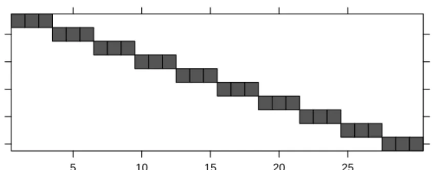
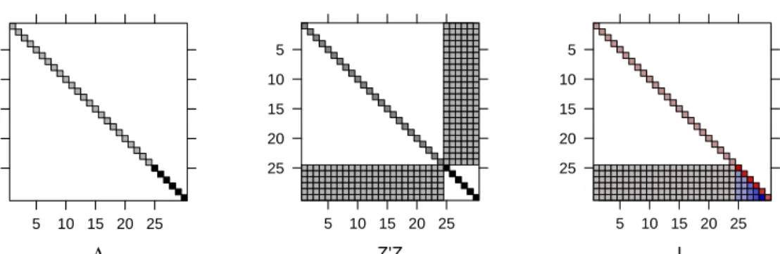
In chapter 1 we saw that a model with a single, simple, scalar random-effects term generated a random-random-effects model matrix, Z, that is the matrix of indicators of the levels of the grouping factor. When we have multiple, simple, scalar random-effects terms, as in model fm2, each term generates a matrix of indicator columns and these sets of indicators are concatenated to form the model matrix Z. The transpose of this matrix, shown in Fig. 2.3, contains rows of indicators for each factor.

The relative covariance factor, Λθ, (Fig. 2.4, left panel) is no longer a

multiple of the identity. It is now block diagonal, with two blocks, one of size 24 and one of size 6, each of which is a multiple of the identity. The diagonal elements of the two blocks are θ1 andθ2, respectively. The numeric values of

these parameters can be obtained as

5 10 15 20 25 50 100

Fig. 2.3 Image of the transpose of the random-effects model matrix, Z, for model

fm2. The non-zero elements, which are all unity, are shown as darkened squares. The zero elements are blank.

Λ 5 10 15 20 25 5 10 15 20 25 Z'Z 5 10 15 20 25 5 10 15 20 25 L 5 10 15 20 25 5 10 15 20 25

Fig. 2.4 Images of the relative covariance factor,Λ, the cross-product of the random-effects model matrix, ZT_{Z, and the sparse Cholesky factor, L, for modelfm2.}

[1] 1.539683 3.512443

The first parameter is the relative standard deviation of the random effects forplate, which has the value0.84671/0.54992=1.53968at convergence, and the second is the relative standard deviation of the random effects for sample

(1.93157/0.54992=3.512443).

Because Λθ is diagonal, the pattern of non-zeros in Λ_θTZTZΛθ +I will be

the same as that in ZT_{Z, shown in the middle panel of Fig. 2.4. The sparse} Cholesky factor, L, shown in the right panel, is lower triangular and has non-zero elements in the lower right hand corner in positions where ZT_{Z has} systematic zeros. We say that “fill-in” has occurred when forming the sparse Cholesky decomposition. In this case there is a relatively minor amount of fill but in other cases there can be a substantial amount of fill and we shall take precautions so as to reduce this, because fill-in adds to the computational effort in determining the MLEs or the REML estimates.

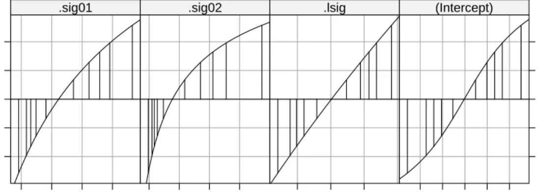
A profile zeta plot (Fig. 2.5) for the parameters in model fm2 leads to con-clusions similar to those from Fig. 1.5 for modelfm1MLin the previous chapter.

The fixed-effect parameter, β0, for the (Intercept)term has symmetric

2.1 A Model With Crossed Random Effects 33 ζ −2 −1 0 1 2 0.6 0.8 1.0 1.2 .sig01 1 2 3 4 .sig02 −0.7 −0.6 −0.5 .lsig 21 22 23 24 25 (Intercept)

Fig. 2.5 Profile zeta plot of the parameters in modelfm2.

of σ has a good normal approximation but the standard deviations of the random effects, σ1 and σ2, are skewed. The skewness for σ2 is worse than

that for σ1, because the estimate of σ2 is less precise than that of σ1, in

both absolute and relative senses. For an absolute comparison we compare the widths of the confidence intervals for these parameters.

> confint(pr2) 2.5 % 97.5 % .sig01 0.6335658 1.1821040 .sig02 1.0957822 3.5563194 .lsig -0.7218645 -0.4629033 (Intercept) 21.2666274 24.6778176

In a relative comparison we examine the ratio of the endpoints of the interval divided by the estimate.

> confint(pr2)[1:2,]/c(0.8455722, 1.770648)

2.5 % 97.5 %

.sig01 0.7492746 1.397993 .sig02 0.6188594 2.008485

The lack of precision in the estimate of σ2 is a consequence of only having

6 distinct levels of the sample factor. The plate factor, on the other hand, has 24 distinct levels. In general it is more difficult to estimate a measure of spread, such as the standard deviation, than to estimate a measure of location, such as a mean, especially when the number of levels of the factor is small. Six levels are about the minimum number required for obtaining sensible estimates of standard deviations for simple, scalar random effects terms.

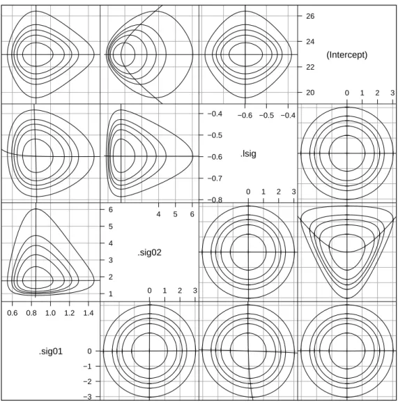
The profile pairs plot (Fig. 2.6) shows patterns similar to those in Fig. 1.9 for pairs of parameters in model fm1 fit to the Dyestuff data. On the ζ scale

Scatter Plot Matrix .sig01 0.6 0.8 1.0 1.2 1.4 −3 −2 −1 0 .sig02 1 2 3 4 5 6 4 5 6 0 1 2 3 .lsig −0.8 −0.7 −0.6 −0.5 −0.4 −0.6 −0.5 −0.4 0 1 2 3 (Intercept) 20 22 24 26 0 1 2 3

Fig. 2.6 Profile pairs plot for the parameters in model fm2 fit to the Penicillin

data.

(panels below the diagonal) the profile traces are nearly straight and orthog-onal with the exception of the trace of ζ(σ2) on ζ(β0) (the horizontal trace

for the panel in the (4,2) position). The pattern of this trace is similar to the pattern of the trace of ζ(σ1) on ζ(β0) in Fig. 1.9. Moving β0 from its

estimate,βb0, in either direction will increase the residual sum of squares. The

increase in the residual variability is reflected in an increase of one or more of the dispersion parameters. The balanced experimental design results in a fixed estimate of σ and the extra apparent variability must be incorporated into σ1 or σ2.

Contours in panels of parameter pairs on the original scales (i.e. panels above the diagonal) can show considerable distortion from the ideal elliptical shape. For example, contours in the σ2 versus σ1 panel (the (1,2) position)

non-2.1 A Model With Crossed Random Effects 35

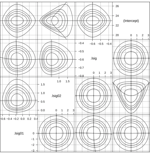
Scatter Plot Matrix .lsig01 −0.6 −0.4 −0.2 0.0 0.2 0.4 −3 −2 −1 0 .lsig02 0.0 0.5 1.0 1.5 1.0 1.5 0 1 2 3 .lsig −0.8 −0.7 −0.6 −0.5 −0.4 −0.6 −0.5 −0.4 0 1 2 3 (Intercept) 20 22 24 26 0 1 2 3

Fig. 2.7 Profile pairs plot for the parameters in model fm2 fit to the Penicillin

data. In this plot the parametersσ1 andσ2 are on the scale of the natural logarithm, as is the parameterσ in this and other profile pairs plots.

elliptical. However, the distortion of the contours is not due to these param-eter estimates depending strongly on each other. It is almost entirely due to the choice of scale for σ1 and σ2. When we plot the contours on the scale of

log(σ1) and log(σ2) instead (Fig. 2.7) they are much closer to the elliptical

pattern.

Conversely, if we tried to plot contours on the scale of σ₁2 and σ₂2 (not shown), they would be hideously distorted.

2.2 A Model With Nested Random Effects

In this section we again consider a simple example, this time fitting a model with nested grouping factors for the random effects.

2.2.1 The

Pastes

Data

The third example from Davies and Goldsmith [1972, Table 6.5, p. 138] is described as coming from

deliveries of a chemical paste product contained in casks where, in addition to sampling and testing errors, there are variations in quality between deliveries . . . As a routine, three casks selected at random from each delivery were sampled and the samples were kept for reference. . . . Ten of the delivery batches were sampled at random and two analytical tests carried out on each of the 30 samples.

The structure and summary of the Pastes data object are > str(Pastes)

'data.frame': 60 obs. of 4 variables:

$ strength: num 62.8 62.6 60.1 62.3 62.7 63.1 60 61.4 57.5 56.9 ... $ batch : Factor w/ 10 levels "A","B","C","D",..: 1 1 1 1 1 1 2 2 2 2.. $ cask : Factor w/ 3 levels "a","b","c": 1 1 2 2 3 3 1 1 2 2 ... $ sample : Factor w/ 30 levels "A:a","A:b","A:c",..: 1 1 2 2 3 3 4 4 5.. > summary(Pastes)

strength batch cask sample

Min. :54.20 A : 6 a:20 A:a : 2

1st Qu.:57.50 B : 6 b:20 A:b : 2 Median :59.30 C : 6 c:20 A:c : 2 Mean :60.05 D : 6 B:a : 2 3rd Qu.:62.88 E : 6 B:b : 2 Max. :66.00 F : 6 B:c : 2 (Other):24 (Other):48

As stated in the description in Davies and Goldsmith [1972], there are 30 samples, three from each of the 10 delivery batches. We have labelled the levels of the sample factor with the label of the batch factor followed

by ‘a’, ‘b’ or ‘c’ to distinguish the three samples taken from that batch. The cross-tabulation produced by thextabsfunction, using the optional argument

sparse = TRUE, provides a concise display of the relationship. > xtabs(~ batch + sample, Pastes, drop = TRUE, sparse = TRUE) 10 x 30 sparse Matrix of class "dgCMatrix"

A 2 2 2 . . . . B . . . 2 2 2 . . . . C . . . 2 2 2 . . . .

2.2 A Model With Nested Random Effects 37 sample batch 2 4 6 8 10 5 10 15 20 25

Fig. 2.8 Image of the cross-tabulation of thebatchandsamplefactors in thePastes

data. D . . . 2 2 2 . . . . E . . . 2 2 2 . . . . F . . . 2 2 2 . . . . G . . . 2 2 2 . . . . H . . . 2 2 2 . . . . I . . . 2 2 2 . . . J . . . 2 2 2

Alternatively, we can use an image (Fig. 2.8) of this cross-tabulation to visu-alize the structure.

When plotting the strength versus batch and samplein the Pastesdata we

should remember that we have two strength measurements on each of the 30 samples. It is tempting to use the cask designation (‘a’, ‘b’ and ‘c’) to determine, say, the plotting symbol within abatch. It would be fine to do this within a batch but the plot would be misleading if we used the same symbol for cask ‘a’ in different batches. There is no relationship between cask ‘a’ in batch ‘A’ and cask ‘a’ in batch ‘B’. The labels ‘a’, ‘b’ and ‘c’ are used only to distinguish the three samples within a batch; they do not have a meaning across batches.

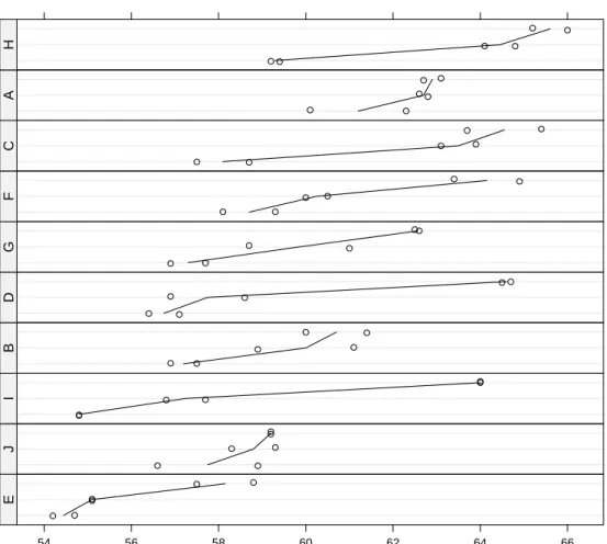
In Fig. 2.9 we plot the two strength measurements on each of the samples within each of the batches and join up the average strength for each sample. The perceptive reader will have noticed that the levels of the factors on the vertical axis in this figure, and in Fig. 1.1 and 2.1, have been reordered ac-cording to increasing average response. In all these cases there is no inherent ordering of the levels of the covariate such asbatchorplate. Rather than

con-fuse our interpretation of the plot by determining the vertical displacement of points according to a random ordering, we impose an ordering according to increasing mean response. This allows us to more easily check for structure in the data, including undesirable characteristics like increasing variability of the response with increasing mean level of the response.

In Fig. 2.9 we order the samples within each batch separately then order the batches according to increasing mean strength.

Paste strength

Sample within batch

E:b E:a E:c 54 56 58 60 62 64 66 ● ● ● ● ● ● E J:c J:a J:b ● ● ● ● ● ● J I:a I:c I:b ● ● ● ● ● ● I B:b B:c B:a ● ● ● ● ● ● B D:a D:b D:c ● ● ● ● ● ● D G:c G:b G:a ●● ● ● ● ● G F:b F:c F:a ● ● ● ● ● ● F C:a C:b C:c ● ● ● ● ● ● C A:b A:a A:c ● ● ● ● ● ● A H:a H:c H:b ● ● ● ● ● ● H

Fig. 2.9 Strength of paste preparations according to thebatchand thesamplewithin the batch. There were two strength measurements on each of the 30 samples; three samples each from 10 batches.

Figure 2.9 shows considerable variability in strength between samples rel-ative to the variability within samples. There is some indication of variability between batches, in addition to the variability induced by the samples, but not a strong indication of a batch effect. For example, batches I and D, with low mean strength relative to the other batches, each contained one sam-ple (I:b and D:c, respectively) that had high mean strength relative to the other samples. Also, batches H and C, with comparatively high mean batch strength, contain samples H:a and C:a with comparatively low mean sample strength. In Sect. 2.2.4 we will examine the need for incorporating batch-to-batch variability, in addition to sample-to-sample variability, in the statistical model.

2.2 A Model With Nested Random Effects 39

2.2.1.1 Nested Factors

Because each level of sample occurs with one and only one level of batch we

say that sample is nested within batch. Some presentations of mixed-effects models, especially those related to multilevel modeling [Rasbash et al., 2000] orhierarchical linear models [Raudenbush and Bryk, 2002], leave the impres-sion that one can only define random effects with respect to factors that are nested. This is the origin of the terms “multilevel”, referring to multiple, nested levels of variability, and “hierarchical”, also invoking the concept of a hierarchy of levels. To be fair, both those references do describe the use of models with random effects associated with non-nested factors, but such models tend to be treated as a special case.

The blurring of mixed-effects models with the concept of multiple, hier-archical levels of variation results in an unwarranted emphasis on “levels” when defining a model and leads to considerable confusion. It is perfectly le-gitimate to define models having random effects associated with non-nested factors. The reasons for the emphasis on defining random effects with respect to nested factors only are that such cases do occur frequently in practice and that some of the computational methods for estimating the parameters in the models can only be easily applied to nested factors.

This is not the case for the methods used in thelme4package. Indeed there is nothing special done for models with random effects for nested factors. When random effects are associated with multiple factors exactly the same computational methods are used whether the factors form a nested sequence or are partially crossed or are completely crossed. A case of a nested sequence of “grouping factors” for the random effects (including the trivial case of only one such factor) is detected but this information does not change the course of the computation. It is available to be used as a diagnostic check. When the user knows that the grouping factors should be nested, she can check if they are indeed nested.

There is, however, one aspect of nested grouping factors that we should emphasize, which is the possibility of a factor that is implicitly nested within another factor. Suppose, for example, that the sample factor was defined as having three levels instead of 30 with the implicit assumption that sample

is nested within batch. It may seem silly to try to distinguish 30 different

batches with only three levels of a factor but, unfortunately, data are fre-quently organized and presented like this, especially in text books. The cask

factor in the Pastes data is exactly such an implicitly nested factor. If we cross-tabulate batch and cask

> xtabs(~ cask + batch, Pastes) batch

cask A B C D E F G H I J a 2 2 2 2 2 2 2 2 2 2 b 2 2 2 2 2 2 2 2 2 2 c 2 2 2 2 2 2 2 2 2 2

we get the impression that thecaskand batchfactors are crossed, not nested.

If we know that the cask should be considered as nested within the batch then we should create a new categorical variable giving the batch-cask combina-tion, which is exactly what thesamplefactor is. A simple way to create such a factor is to use the interaction operator, ‘:’, on the factors. It is advisable, but

not necessary, to apply factorto the result thereby dropping unused levels of

the interaction from the set of all possible levels of the factor. (An “unused level” is a combination that does not occur in the data.) A convenient code idiom is

> Pastes$sample <- with(Pastes, factor(batch:cask))

or

> Pastes <- within(Pastes, sample <- factor(batch:cask))

In a small data set like Pastes we can quickly detect a factor being implic-itly nested within another factor and take appropriate action. In a large data set, perhaps hundreds of thousands of test scores for students in thousands of schools from hundreds of school districts, it is not always obvious if school identifiers are unique across the entire data set or just within a district. If you are not sure, the safest thing to do is to create the interaction factor, as shown above, so you can be confident that levels of the district:school interaction do indeed correspond to unique schools.

2.2.2 Fitting a Model With Nested Random Effects

Fitting a model with simple, scalar random effects for nested factors is done in exactly the same way as fitting a model with random effects for crossed grouping factors. We include random-effects terms for each factor, as in

> (fm3 <- lmer(strength ~ 1 + (1|sample) + (1|batch), Pastes, REML=0)) Linear mixed model fit by maximum likelihood

Formula: strength ~ 1 + (1 | sample) + (1 | batch) Data: Pastes

AIC BIC logLik deviance

256 264.4 -124 248

Random effects:

Groups Name Variance Std.Dev.

sample (Intercept) 8.4337 2.9041

batch (Intercept) 1.1992 1.0951

Residual 0.6780 0.8234

Number of obs: 60, groups: sample, 30; batch, 10 Fixed effects:

Estimate Std. Error t value

2.2 A Model With Nested Random Effects 41 Λ 10 20 30 10 20 30 Z'Z 10 20 30 10 20 30 L 10 20 30 10 20 30

Fig. 2.10 Images of the relative covariance factor, Λ, the cross-product of the random-effects model matrix, ZT_{Z, and the sparse Cholesky factor, L, for model}

fm3.

Not only is the model specification similar for nested and crossed factors, the internal calculations are performed according to the methods described in Sect. 1.4.1 for each model type. Comparing the patterns in the matricesΛ,

ZT_{Z and L for this model (Fig. 2.10) to those in Fig. 2.4 shows that models} with nested factors produce simple repeated structures along the diagonal of the sparse Cholesky factor,L, after reordering the random effects (we discuss this reordering later in Sect. 5.4.1). This type of structure has the desirable property that there is no “fill-in” during calculation of the Cholesky factor. In other words, the number of non-zeros in L is the same as the number of non-zeros in the lower triangle of the matrix being factored, ΛT_ZT_{ZΛ +I} (which, becauseΛ is diagonal, has the same structure as ZT_Z).

Fill-in of the Cholesky factor is not an important issue when we have a few dozen random effects, as we do here. It is an important issue when we have millions of random effects in complex configurations, as has been the case in some of the models that have been fit using lmer.

2.2.3 Assessing Parameter Estimates in Model

fm3

The parameter estimates are: σc1=2.904, the standard deviation of the

ran-dom effects forsample;cσ2=1.095, the standard deviation of the random effects

for batch; σb =0.823, the standard deviation of the residual noise term; and

b

β0=60.053, the overall mean response, which is labeled (Intercept) in these

models.

The estimated standard deviation for sampleis nearly three times as large

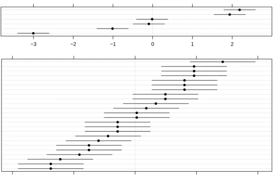
con-I:a E:b E:a D:a G:cB:b C:aI:c D:bJ:c H:aF:b J:a E:cJ:b G:bF:c B:c A:b B:a A:a A:c G:aC:b H:c F:a C:cI:b D:c H:b −5 0 5 ● ● ● ● ● ● ● ● ● ● ● ● ● ● ● ● ● ● ● ● ● ● ● ● ● ● ● ● ● ● EJ I B D GF CA H −3 −2 −1 0 1 2 ● ● ● ● ● ● ● ● ● ●

Fig. 2.11 95% prediction intervals on the random effects for model fm3 fit to the

Pastesdata.

clusion from Fig. 2.9 was that there may not be a significant batch-to-batch variability in addition to the sample-to-sample variability.

Plots of the prediction intervals of the random effects (Fig. 2.11) confirm this impression in that all the prediction intervals for the random effects for

batch contain zero. Furthermore, the profile zeta plot (Fig. 2.12) shows that the even the 50% profile-based confidence interval on σ2 extends to zero.

Because there are several indications that σ2 could reasonably be zero,

resulting in a simpler model incorporating random effects for batch only, we

perform a statistical test of this hypothesis.

2.2.4 Testing

H

:

σ

=

0

Versus

H

:

σ

>

0

One of the many famous statements attributed to Albert Einstein is “Every-thing should be made as simple as possible, but not simpler.” In statistical modeling thisprincipal of parsimony is embodied in hypothesis tests compar-ing two models, one of which contains the other as a special case. Typically,

2.2 A Model With Nested Random Effects 43 ζ −2 −1 0 1 2 2.0 2.5 3.0 3.5 4.0 4.5 .sig01 0 1 2 3 .sig02 −0.4 −0.2 0.0 0.2 .lsig 58 59 60 61 62 (Intercept)

Fig. 2.12 Profile zeta plots for the parameters in model fm3.

one or more of the parameters in the more general model, which we call the

alternative hypothesis, is constrained in some way, resulting in the restricted model, which we call the null hypothesis. Although we phrase the hypothesis test in terms of the parameter restriction, it is important to realize that we are comparing the quality of fits obtained with two nested models. That is, we are not assessing parameter values per se; we are comparing the model fit obtainable with some constraints on parameter values to that without the constraints.

Because the more general model, Ha, must provide a fit that is at least as

good as the restricted model, H0, our purpose is to determine whether the

change in the quality of the fit is sufficient to justify the greater complexity of model Ha. This comparison is often reduced to a p-value, which is the

probability of seeing a difference in the model fits as large as we did, or even larger, when, in fact, H0 is adequate. Like all probabilities, a p-value must

be between 0 and 1. When the p-value for a test is small (close to zero) we prefer the more complex model, saying that we “reject H0 in favor of Ha”. On

the other hand, when the p-value is not small we “fail to reject H0”, arguing

that there is a non-negligible probability that the observed difference in the model fits could reasonably be the result of random chance, not the inherent superiority of the modelHa. Under these circumstances we prefer the simpler

model, H0, according to the principal of parsimony.

These are the general principles of statistical hypothesis tests. To perform a test in practice we must specify the criterion for comparing the model fits, the method for calculating the p-value from an observed value of the criterion, and the standard by which we will determine if the p-value is “small” or not. The criterion is called the test statistic, the p-value is calculated from a reference distribution for the test statistic, and the standard for small p-values is called the level of the test.

In Sect. 1.5 we referred to likelihood ratio tests (LRTs) for which the test statistic is the difference in the deviance. That is, the LRT statistic isd0−da

where da is the deviance in the more general (Ha) model fit and d0 is the

de-viance in the constrained (H0) model. An approximate reference distribution

for an LRT statistic is the χ2

ν distribution where ν, the degrees of freedom,

is determined by the number of constraints imposed on the parameters of Ha

to produce H0.

The restricted model fit

> (fm3a <- lmer(strength ~ 1 + (1|sample), Pastes, REML=0)) Linear mixed model fit by maximum likelihood

Formula: strength ~ 1 + (1 | sample) Data: Pastes

AIC BIC logLik deviance

254.4 260.7 -124.2 248.4

Random effects:

Groups Name Variance Std.Dev.

sample (Intercept) 9.6328 3.1037

Residual 0.6780 0.8234

Number of obs: 60, groups: sample, 30 Fixed effects:

Estimate Std. Error t value

(Intercept) 60.0533 0.5765 104.2

is compared to model fm3 with the anova function > anova(fm3a, fm3)

Data: Pastes Models:

fm3a: strength ~ 1 + (1 | sample)

fm3: strength ~ 1 + (1 | sample) + (1 | batch)

Df AIC BIC logLik Chisq Chi Df Pr(>Chisq)

fm3a 3 254.40 260.69 -124.20

fm3 4 255.99 264.37 -124.00 0.4072 1 0.5234

which provides a p-value of 0.5234. Because typical standards for “small” p-values are 5% or 1%, a p-value over 50% would not be considered significant at any reasonable level.

We do need to be cautious in quoting this p-value, however, because the parameter value being tested, σ2=0, is on the boundary of set of possible

values, σ2≥0, for this parameter. The argument for using a χ₁2 distribution

to calculate a p-value for the change in the deviance does not apply when the parameter value being tested is on the boundary. As shown in Pinheiro and Bates [2000, Sect. 2.5], the p-value from the χ2

1 distribution will be

“conser-vative” in the sense that it is larger than a simulation-based p-value would be. In the worst-case scenario the χ2_{-based p-value will be twice as large as}

it should be but, even if that were true, an effective p-value of 26% would not cause us to reject H0 in favor of Ha.

2.3 A Model With Partially Crossed Random Effects 45 ζ −2 −1 0 1 2 2.5 3.0 3.5 4.0 4.5 .sig01 −0.4 −0.2 0.0 0.2 .lsig 59 60 61 (Intercept)

Fig. 2.13 Profile zeta plots for the parameters in model fm3a.

2.2.5 Assessing the Reduced Model,

fm3a

The profile zeta plots for the remaining parameters in model fm3a (Fig. 2.13)

are similar to the corresponding panels in Fig. 2.12, as confirmed by the numerical values of the confidence intervals.

> confint(pr3) 2.5 % 97.5 % .sig01 2.1579337 4.05358895 .sig02 NA 2.94658928 .lsig -0.4276761 0.08199287 (Intercept) 58.6636504 61.44301637 > confint(pr3a) 2.5 % 97.5 % .sig01 2.4306377 4.12201052 .lsig -0.4276772 0.08199277 (Intercept) 58.8861831 61.22048353

The confidence intervals on log(σ) and β0 are similar for the two models.

The confidence interval on σ1 is slightly wider in model fm3a than in fm3,

because the variability that is attributed to batch in fm3 is incorporated into the variability due to sample infm3a.

The patterns in the profile pairs plot (Fig. 2.14) for the reduced model

fm3a are similar to those in Fig. 1.9, the profile pairs plot for model fm1.

2.3 A Model With Partially Crossed Random Effects

Scatter Plot Matrix .sig01 2.5 3.0 3.5 4.0 4.5 5.0 −3 −2 −1 0 .lsig −0.4 −0.2 0.0 0.2 0.0 0.2 0 1 2 3 (Intercept) 58 59 60 61 62 0 1 2 3

Fig. 2.14 Profile pairs plot for the parameters in modelfm3afit to thePastesdata.

crossed. We describe such situations as havingpartially crossed grouping fac-tors for the random effects.

Studies in education, in which test scores for students over time are also associated with teachers and schools, usually result in partially crossed group-ing factors. If students with scores in multiple years have different teachers for the different years, the student factor cannot be nested within the teacher factor. Conversely, student and teacher factors are not expected to be com-pletely crossed. To have complete crossing of the student and teacher factors it would be necessary for each student to be observed with each teacher, which would be unusual. A longitudinal study of thousands of students with hundreds of different teachers inevitably ends up partially crossed.

In this section we consider an example with thousands of students and instructors where the response is the student’s evaluation of the instructor’s effectiveness. These data, like those from most large observational studies, are quite unbalanced.

2.3 A Model With Partially Crossed Random Effects 47

2.3.1 The

InstEval

Data

TheInstEvaldata are from a special evaluation of lecturers by students at the Swiss Federal Institute for Technology–Z¨urich (ETH–Z¨urich), to determine who should receive the “best-liked professor” award. These data have been slightly simplified and identifying labels have been removed, so as to preserve anonymity.

The variables

> str(InstEval)

'data.frame': 73421 obs. of 7 variables:

$ s : Factor w/ 2972 levels "1","2","3","4",..: 1 1 1 1 2 2 3 3 3 .. $ d : Factor w/ 1128 levels "1","6","7","8",..: 525 560 832 1068 6.. $ studage: Ord.factor w/ 4 levels "2"<"4"<"6"<"8": 1 1 1 1 1 1 1 1 1 1 .. $ lectage: Ord.factor w/ 6 levels "1"<"2"<"3"<"4"<..: 2 1 2 2 1 1 1 1 1.. $ service: Factor w/ 2 levels "0","1": 1 2 1 2 1 1 2 1 1 1 ...

$ dept : Factor w/ 14 levels "15","5","10",..: 14 5 14 12 2 2 13 3 3 ..

$ y : int 5 2 5 3 2 4 4 5 5 4 ...

have somewhat cryptic names. Factor s designates the student and d the

instructor. Thedeptfactor is the department for the course and service indi-cates whether the course was a service course taught to students from other departments.

Although the response, y, is on a scale of 1 to 5, > xtabs(~ y, InstEval)

y

1 2 3 4 5

10186 12951 17609 16921 15754

it is sufficiently diffuse to warrant treating it as if it were a continuous re-sponse.

At this point we will fit models that have random effects for student, instructor, and department (or the dept:service combination) to these data.

In the next chapter we will fit models incorporating fixed-effects for instructor and department to these data.

> (fm4 <- lmer(y ~ 1 + (1|s) + (1|d)+(1|dept:service), InstEval, REML=0)) Linear mixed model fit by maximum likelihood

Formula: y ~ 1 + (1 | s) + (1 | d) + (1 | dept:service) Data: InstEval

AIC BIC logLik deviance

237663 237709 -118827 237653

Random effects:

Groups Name Variance Std.Dev.

s (Intercept) 0.105404 0.32466

d (Intercept) 0.262563 0.51241

dept:service (Intercept) 0.012126 0.11012

6:1 11:1 10:0 9:1 14:12:1 15:07:1 12:1 1:0 3:0 2:0 1:1 12:0 8:0 3:1 6:0 5:0 9:0 14:0 10:1 4:1 11:0 5:1 7:0 4:0 8:1 15:1 −0.5 0.0 0.5 ● ● ● ● ● ● ● ● ● ● ● ● ● ● ● ● ● ● ● ● ● ● ● ● ● ● ● ●

Fig. 2.15 95% prediction intervals on the random effects for thedept:servicefactor in model fm4 fit to theInstEval data.

Number of obs: 73421, groups: s, 2972; d, 1128; dept:service, 28 Fixed effects:

Estimate Std. Error t value

(Intercept) 3.25521 0.02824 115.3

(Fitting this complex model to a moderately large data set takes less than two minutes on a modest laptop computer purchased in 2006. Although this is more time than required for earlier model fits, it is a remarkably short time for fitting a model of this size and complexity. In some ways it is remarkable that such a model can be fit at all on such a computer.)

All three estimated standard deviations of the random effects are less than

b

σ, with σb3, the estimated standard deviation of the random effects for the

dept:service interaction, less than one-tenth the estimated residual standard deviation.

It is not surprising that zero is within all of the prediction intervals on the random effects for this factor (Fig. 2.15). In fact, zero is close to the middle of all these prediction intervals. However, the p-value for the LRT ofH0:σ3=0

versus Ha:σ3>0

> fm4a <- lmer(y ~ 1 + (1|s) + (1|d), InstEval, REML=0) > anova(fm4a,fm4)

Data: InstEval Models:

fm4a: y ~ 1 + (1 | s) + (1 | d)

2.3 A Model With Partially Crossed Random Effects 49

Fig. 2.16 Image of the sparse Cholesky factor, L, from modelfm4

Df AIC BIC logLik Chisq Chi Df Pr(>Chisq)

fm4a 4 237786 237823 -118889

fm4 5 237663 237709 -118827 124.43 1 < 2.2e-16

is highly significant. That is, we have very strong evidence that we should reject H0 in favor of Ha.

The seeming inconsistency of these conclusions is due to the large sample size (n=73421). When a model is fit to a very large sample even the most subtle of differences can be highly “statistically significant”. The researcher or data analyst must then decide if these terms have practical significance, beyond the apparent statistical significance.

The large sample size also helps to assure that the parameters have good normal approximations. We could profile this model fit but doing so would take a very long time and, in this particular case, the analysts are more interested in a model that uses fixed-effects parameters for the instructors, which we will describe in the next chapter.

We could pursue other mixed-effects models here, such as using the dept

factor and not the dept:service interaction to define random effects, but we will revisit these data in the next chapter and follow up on some of these variations there.

2.3.2 Structure of

L

for model

fm4

Before leaving this model we examine the sparse Cholesky factor,L, (Fig. 2.16), which is of size 4128×4128. Even as a sparse matrix this factor requires a considerable amount of memory,

> object.size(env(fm4)$L) 6904640 bytes

> unclass(round(object.size(env(fm4)$L)/2^20, 3)) # size in megabytes [1] 6.585

but as a triangular dense matrix it would require nearly 10 times as much. There are (4128×4129)/2elements on and below the diagonal, each of which would require 8 bytes of storage. A packed lower triangular array would re-quire

> (8 * (4128 * 4129)/2)/2^20 # size in megabytes [1] 65.01965

megabytes. The more commonly used full rectangular storage requires

> (8 * 4128^2)/2^20 # size in megabytes [1] 130.0078

megabytes of storage.

The number of nonzero elements in this matrix that must be updated for each evaluation of the deviance is

> nnzero(as(env(fm4)$L, "sparseMatrix")) [1] 566960

Comparing this to 8522256, the number of elements that must be updated in a dense Cholesky factor, we can see why the sparse Cholesky factor provides a much more efficient evaluation of the profiled deviance function.

2.4 Chapter Summary

A simple, scalar random effects term in anlmer model formula is of the form

(1|fac), where fac is an expression whose value is the grouping factor of the

set of random effects generated by this term. Typically,facis simply the name

of a factor, such as in the terms (1|sample) or (1|plate) in the examples in this chapter. However, the grouping factor can be the value of an expression, such as (1|dept:service) in the last example.

2.4 Chapter Summary 51

Because simple, scalar random-effects terms can differ only in the descrip-tion of the grouping factor we refer to configuradescrip-tions such as crossed or nested as applying to the terms or to the random effects, although it is more accurate to refer to the configuration as applying to the grouping factors.

A model formula can include several such random effects terms. Because configurations such as nested or crossed or partially crossed grouping factors are a property of the data, the specification in the model formula does not depend on the configuration. We simply include multiple random effects terms in the formula specifying the model.

One apparent exception to this rule occurs with implicitly nested factors, in which the levels of one factor are only meaningful within a particular level of the other factor. In the Pastes data, levels of the cask factor are only

meaningful within a particular level of the batch factor. A model formula of strength ~ 1 + (1 | cask) + (1 | batch)

would result in a fitted model that did not appropriately reflect the sources of variability in the data. Following the simple rule that the factor should be defined so that distinct experimental or observational units correspond to distinct levels of the factor will avoid such ambiguity.

For convenience, a model with multiple, nested random-effects terms can be specified as

strength ~ 1 + (1 | batch/cask)

which internally is re-expressed as

strength ~ 1 + (1 | batch) + (1 | batch:cask)

We will avoid terms of the form (1|batch/cask), preferring instead an

ex-plicit specification with simple, scalar terms based on unambiguous grouping factors.

The InstEval data, described in Sec. 2.3.1, illustrate some of the

charac-teristics of the real data to which mixed-effects models are now fit. There is a large number of observations associated with several grouping factors; two of which, student and instructor, have a large number of levels and are partially crossed. Such data are common in sociological and educational studies but until now it has been very difficult to fit models that appropriately reflect such a structure. Much of the literature on mixed-effects models leaves the impression that multiple random effects terms can only be associated with nested grouping factors. The resulting emphasis on hierarchical or multilevel configurations is an artifact of the computational methods used to fit the models, not the models themselves.

The parameters of the models fit to small data sets have properties similar to those for the models in the previous chapter. That is, profile-based confi-dence intervals on the fixed-effects parameter, β0, are symmetric about the

estimate but overdispersed relative to those that would be calculated from a normal distribution and the logarithm of the residual standard deviation, log(σ), has a good normal approximation. Profile-based confidence intervals

for the standard deviations of random effects (σ1, σ2, etc.) are symmetric on

a logarithmic scale except for those that could be zero.

Another observation from the last example is that, for data sets with a very large numbers of observations, a term in a model may be “statistically significant” even when its practical significance is questionable.

Exercises

These exercises use data sets from the MEMSS package for R. Recall that to

access a particular data set, you must either attach the package

> library(MEMSS)

or load just the one data set

> data(ergoStool, package = "MEMSS")

We begin with exercises using the ergoStool data from the MEMSS package.

The analysis and graphics in these exercises is performed in Chap. 3. The purpose of these exercises is to see if you can use the material from this chapter to anticipate the results quoted in the next chapter.

2.1. Check the documentation, the structure (str) and a summary of the ergoStool data from the MEMSS package. (If you are familiar with the Star Trek television series and movies, you may want to speculate about what, exactly, the “Borg scale” is.) Use

> xtabs(~ Type + Subject, ergoStool)

to determine if these factors are nested, partially crossed or completely crossed. Is this a replicated or an unreplicated design?

2.2. Create a plot, similar to Fig. 2.1, showing the effort by subject with lines connecting points corresponding to the same stool types. Order the levels of the Subject factor by increasing average effort.

2.3. The experimenters are interested in comparing these specific stool types. In the next chapter we will fit a model with fixed-effects for the Type factor

and random effects for Subject, allowing us to perform comparisons of these specific types. At this point fit a model with random effects for both Type

and Subject. What are the relative sizes of the estimates of the standard

deviations,σb1 (forSubject), σb2 (forType) andσb (for the residual variability)?

2.4. Refit the model using maximum likelihood. Check the parameter esti-mates and, in the case of the fixed-effects parameter, β0, its standard error.

In what ways have the parameter estimates changed? Which parameter esti-mates have not changed?

2.4 Chapter Summary 53

2.5. Profile the fitted model and construct 95% profile-based confidence in-tervals on the parameters. (Note that you will get the same profile object whether you start with the REML fit or the ML fit. There is a slight advan-tage in starting with the ML fit.) Is the confidence interval on σ1 close to

being symmetric about its estimate? Is the confidence interval on σ2 close to

being symmetric about its estimate? Is the corresponding interval onlog(σ1)

close to being symmetric about its estimate?

2.6. Create the profile zeta plot for this model. For which parameters are there good normal approximations?

2.7. Create a profile pairs plot for this model. Comment on the shapes of the profile traces in the transformed (ζ) scale and the shapes of the contours in the original scales of the parameters.

2.8. Create a plot of the 95% prediction intervals on the random effects for

Type using

> dotplot(ranef(fm, which = "Type", postVar = TRUE), aspect = 0.2,

+ strip = FALSE)

(Substitute the name of your fitted model for fmin the call to ranef.) Is there

a clear winner among the stool types? (Assume that lower numbers on the Borg scale correspond to less effort).

2.9. Create a plot of the 95% prediction intervals on the random effects for

Subject.

2.10. Check the documentation, the structure (str) and a summary of the Meatdata from the MEMSS package. Use a cross-tabulation to discover whether Pair and Block are nested, partially crossed or completely crossed.

2.11. Use a cross-tabulation

> xtabs(~ Pair + Storage, Meat)

to determine whether Pair and Storage are nested, partially crossed or com-pletely crossed.

2.12. Fit a model of the score in the Meat data with random effects for Pair, Storage and Block.

2.13. Plot the prediction intervals for each of the three sets of random effects.

2.14. Profile the parameters in this model. Create a profile zeta plot. Does including the random effect forBlock appear to be warranted. Does your con-clusion from the profile zeta plot agree with your concon-clusion from examining the prediction intervals for the random effects for Block?

2.15. Refit the model without random effects forBlock. Perform a likelihood

ratio test of H0:σ3 =0 versus Ha :σ3 >0. Would you reject H0 in favor of

Ha or fail to rejectH0? Would you reach the same conclusion if you adjusted

the p-value for the test by halving it, to take into account the fact that 0 is on the boundary of the parameter region?

2.16. Profile the reduced model (i.e. the one without random effects forBlock)

and create profile zeta and profile pairs plots. Can you explain the apparent interaction between log(σ) and σ1? (This is a difficult question.)