UCLA
UCLA Electronic Theses and Dissertations
TitleOn the Performance and Linear Convergence of Decentralized Primal-Dual Methods Permalink https://escholarship.org/uc/item/1p19x685 Author Alghunaim, Sulaiman A Publication Date 2020 Peer reviewed|Thesis/dissertation
UNIVERSITY OF CALIFORNIA Los Angeles
On the Performance and Linear Convergence of Decentralized Primal-Dual Methods
A dissertation submitted in partial satisfaction of the requirements for the degree
Doctor of Philosophy in Electrical and Computer Engineering
by
c
Copyright by
Sulaiman A. Alghunaim 2020
ABSTRACT OF THE DISSERTATION
On the Performance and Linear Convergence of Decentralized Primal-Dual Methods
by
Sulaiman A. Alghunaim
Doctor of Philosophy in Electrical and Computer Engineering University of California, Los Angeles, 2020
Professor Ali H. Sayed, Chair
This dissertation studies the performance and linear convergence properties of primal-dual methods for the solution of decentralized multi-agent optimization problems. Decentralized multi-agent optimization is a powerful paradigm that finds applications in diverse fields in learning and engineering design. In these setups, a network of agents is connected through some topology and agents are allowed to share information only locally. Their overall goal is to seek the minimizer of a global optimization problem through localized interactions. In decentralized consensus problems, the agents are coupled through a common consensus variable that they need to agree upon. While in decentralized resource allocation problems, the agents are coupled through global affine constraints.
Various decentralized consensus optimization algorithms already exist in the literature. Some methods are derived from a primal-dual perspective, while other methods are derived as gradient tracking mechanisms meant to track the average of local gradients. Among the gradient tracking methods are the adapt-then-combine implementations motivated by diffusion strategies, which have been observed to perform better than other implementations. In this dissertation, we develop a noveladapt-then-combineprimal-dual algorithmic framework that captures most state-of-the-art gradient based methods as special cases including all the variations of the gradient-tracking methods. We also develop a concise and novel analysis
convex objectives. Due to our unified framework, the analysis reveals important characteristics for these methods such as their convergence rates and step-size stability ranges. Moreover, the analysis reveals how the augmented Lagrangian penalty term, which is utilized in most of these methods, affects the performance of decentralized algorithms.
Another important question that we answer is whether decentralized proximal gradient methods can achieve global linear convergence for non-smoothcomposite optimization. For centralized algorithms, linear convergence has been established in the presence of a non-smooth composite term. In this dissertation, we close the gap between centralized and decentralized proximal gradient algorithms and show that decentralized proximal algorithms can also achieve linear convergence in the presence of a non-smooth term. Furthermore, we show that when each agent possesses a differentlocal non-smooth term then global linear convergence cannot be established in the worst case.
Most works that study decentralized optimization problems assume that all agents are involved in computing all variables. However, in many applications the coupling across agents is sparse in the sense that only a few agents are involved in computing certain variables. We show how to design decentralized algorithms in sparsely coupled consensus and resource allocation problems. More importantly, we establish analytically the importance of exploiting the sparsity structure in coupled large-scale networks.
The dissertation of Sulaiman A. Alghunaim is approved. Abeer Alwan Robert M’Closkey Lieven Vandenberghe Ali H. Sayed, Committee Chair
University of California, Los Angeles 2020
TABLE OF CONTENTS
List of Figures . . . x
List of Tables . . . xii
Acknowledgments . . . xiii
Vita . . . xiv
1 Introduction . . . 1
1.1 Multi-Agent Optimization . . . 1
1.2 Decentralized Consensus Optimization . . . 2
1.3 Decentralized Resource Sharing Optimization . . . 5
1.4 Outline and Contributions . . . 6
Appendices . . . 9
1.A Notation . . . 9
1.B Network Combination Weights . . . 10
1.C Optimization Background . . . 11
2 Primal-Dual Gradient Methods. . . 14
2.1 Problem Set-up . . . 14
2.1.1 Related Works . . . 15
2.1.2 Contribution . . . 17
2.2 Convergence Results . . . 17
2.A Proof of Theorem 2.1 . . . 21
2.B Proof of Corollary 2.1 . . . 24
3 Decentralized Primal-Dual Algorithms . . . 25
3.1 Decentralized Optimization Set-up . . . 25
3.1.1 Related Works . . . 26
3.1.2 Contribution . . . 27
3.2 Adapt-then-Combine Framework . . . 28
3.2.1 General Primal-Dual Algorithm . . . 28
3.2.2 Network Combination Matrix . . . 29
3.2.3 Specific Decentralized Algorithms . . . 30
3.3 Convergence Results . . . 34
3.4 Influence of Augmented Lagrangian Term . . . 39
3.5 Numerical Simulations . . . 41
Appendices . . . 45
3.A Equivalent Representation . . . 45
3.A.1 Aug-DGM (ATC-DIGing) . . . 45
3.A.2 ATC-Tracking I . . . 45
3.A.3 ATC-Tracking II . . . 46
3.B Proof of Lemma 3.2 . . . 46
3.C Proof of Theorem 3.1 . . . 48
3.D Proof of Theorem 3.2 . . . 49
4 Decentralized Proximal Primal-dual Algorithms . . . 51
4.1.1 Related Work . . . 52
4.1.2 Contribution . . . 54
4.2 Proximal ATC Algorithms . . . 55
4.3 Linear Convergence . . . 56
4.4 Separate non-smooth terms: Sublinear rate . . . 58
4.5 Simulations . . . 61
4.5.1 Simulations of the Proposed Method . . . 61
4.5.2 Numerical counter example . . . 64
Appendices . . . 64
4.A Proof of Lemma 4.1 . . . 64
4.B Implementation of (4.8) . . . 67
4.B.1 Prox-ED: A¯= 0.5(I+A), B2 = 0.5(I− A), and C = 0 . . . . 67
4.B.2 Prox-ATC I: A¯=A2, B2 = (I− A)2, and C = 0 . . . . 68
4.B.3 Prox-ATC II: A¯=A, B=I− A, and C =I− A . . . 69
4.C Proof Theorem 4.1 . . . 70
4.D Proximal mapping of (4.19) . . . 72
5 Multi-Coupled Consensus Problem . . . 73
5.1 Problem Set-Up . . . 73
5.1.1 Related works . . . 77
5.1.2 Contribution . . . 78
5.2 Problem Reformulation for Decentralized Solution . . . 78
5.3 Cluster Combination Matrices . . . 80
6 Multi-Coupled Resource Sharing Problem . . . 89 6.1 Motivation . . . 89 6.2 Problem Setup . . . 93 6.2.1 Related Works . . . 95 6.2.2 Main Contributions . . . 97 6.3 Algorithm Development . . . 98 6.3.1 Dual Problem . . . 99 6.3.2 Combination Coefficients . . . 101
6.3.3 Dual Coupled Diffusion . . . 101
6.4 Network Recursion . . . 103
6.5 Convergence Results . . . 106
6.6 Numerical Simulation . . . 111
Appendices . . . 116
6.A Equivalent Representation . . . 116
6.B Primal Error Bound . . . 117
6.C Dual Error Bound . . . 119
6.D Proof of Theorem 6.1 . . . 122
6.E Proof of Theorem 6.2 . . . 124
7 Conclusion and Future Directions . . . 128
LIST OF FIGURES
1.1 Centralized vs decentralized networks. . . 2
3.1 Simulation results illustrating the influence of the AL term. . . 44
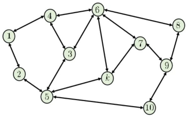
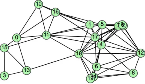
4.1 The network topology used in the simulation. . . 62 4.2 Simulation results. The y-axis indicates the relative squared error PK
k=1kwk,i−
w?k2/kw?k2. Prox-ED refers to (4.8) withA¯= 0.5(I+A), B2 = 0.5(I − A), and C = 0. Prox-ATC I refers to (4.8) withA¯= A2,B= I− A, andC = 0. Prox-ATC
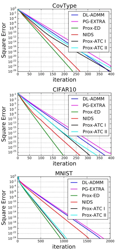
II refers to (4.8) with A¯ = A, B = I − A, and C = I − A. DL-ADMM [53], PG-EXTRA [129], NIDS [56]. . . 63 4.3 Both PG-EXTRA [129] and DL-ADMM [53, 128] converge sublinearly to the
solution of the proposed numerical counter example. . . 65
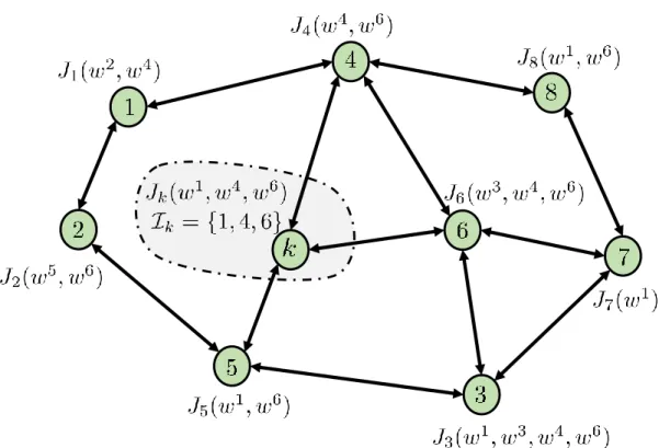
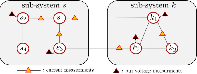
5.1 A connected network of agents where different agents generally depend on different subsets of parameter vectors. For this example, we have w= [w1, w2, w3, w4, w5, w6]. 74 5.2 Two neighboring sub-systems sharing states across their interconnection, i.e., buses
k1-s1 and k3-s3. . . 76
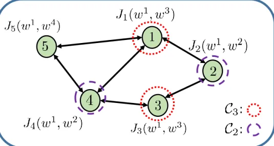
5.3 A five-agent network with unconnected C2 andC3. . . 81
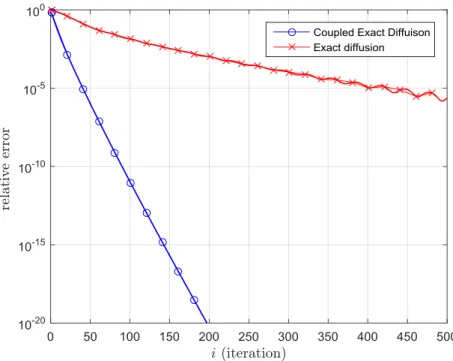
5.4 Network topology used in the simulation results. . . 88 5.5 Relative errors for the coupled diffusion and the exact diffusion algorithms. . . . 88
6.1 An illustration for Example 6.2. In this illustration, there areE = 3areas andK = 6
agents. . . 92 6.2 An example to illustrate the dual problem (6.17) for agentk= 4. In this example we have
three sub-networks and agent 4 is involved in the equality constraints for sub-networks
6.3 An illustration of constructions (6.25) and (6.26) for the network in Figure 6.2 as well as construction (6.32) for agent k= 4 in that network.. . . 104
6.4 Simulation results. *Dual diffusion refers to (6.24) applied on the same problem reformu-lated into (6.1), which ignores the sparsity structure. Similarly, both IDC-ADMM [53] and "dual DIGing" [174] are designed for problem (6.1) and ignore the sparsity structure.113 6.5 A comparison of algorithm (6.24) for different network connectivity and under two
implementations: dual coupled diffusion exploits structure while dual diffusion ignores the structure. . . 115 6.6 An illustration of the construction B for the network in Figure 6.2. . . 124
LIST OF TABLES
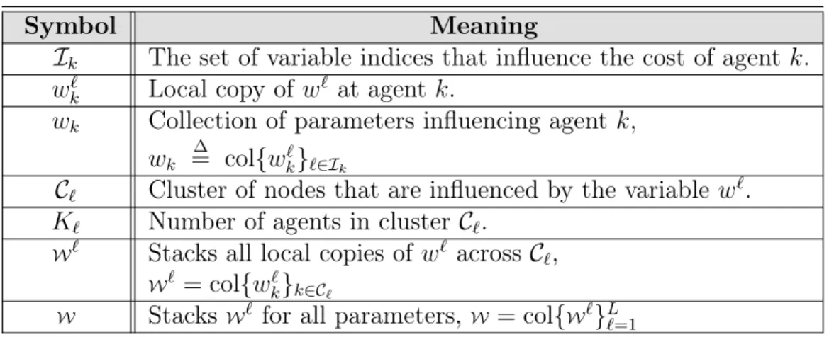
5.1 A listing of the main symbols used in this chapter . . . 80
ACKNOWLEDGMENTS
First and foremost, all praise be to Allah (God).
I would like to express my gratitude to my adviser professor Ali H. Sayed for giving me the opportunity to work under his supervision at the Adaptive System Laboratory at UCLA. Professor Sayed’s patience with me in research has greatly improved the quality of my work. Through our interactions, I have learned many valuable lessons from him whether directly said or indirectly through his high standards and passion in work. I am sure that these lessons will stick with me forever.
I am grateful to all my committee members, Professor Abeer Alwan, Professor Robert M’Closkey, and Professor Lieven Vandenberghe. I thank them for their time spent serving on my committee.
I would like to thank Ryo Arreola and Deeona Columbia for their help during my time at UCLA. At UCLA, I have met many colleagues, visitors, and collaborators: Lucas Cassano, Kun Yuan, Bicheng Ying, Stefan Vlaski, Hawraa Salami, Chung-Kai Yu, Ernest K. Ryu, Chengcheng Wang, Edward Nguyen, and Professor João Y. Ishihara. I am sure that I have learned a lot from them through our discussions and chats. I also cannot forget the people I met during my visit to EPFL: Patricia Vonlanthen, Roula Nassif, Guillermo Ortiz Jimenez, Professor Ricardo Merched, Augusto Santos, Elsa Rizk, and Virginia Bordignon.
Without a doubt this experience would have been much harder if not for the support of my family especially my mother for her belief in me and my wife for being on my side. During my studies, I met with many friends, I thank all of them for all the enjoyable moments we spent in LA.
Finally, I would like to thank Kuwait University for supporting my studies and I am forever grateful to them.
VITA
2013 B.S. in Electrical Engineering, Kuwait University, Kuwait.
2013-2014 Data Core Engineer, Huawei Telecommunication, Kuwait
2016 M.S. in Electrical Engineering, University of California, Los Angeles.
2018 Visiting Student EPFL, Switzerland
PUBLICATIONS
• S. A. Alghunaim and A. H. Sayed, “Linear convergence of primal-dual gradient methods and their performance in distributed optimization," submitted for publication, 2019.
• S. A. Alghunaim, Ernest K. Ryu, K. Yuan, and A. H. Sayed, “Decentralized proximal gradient algorithms with linear convergence rates," conditionally accepted in IEEE Trans. Automatic Control.
• S. A. Alghunaim, K. Yuan, and A. H. Sayed, “A proximal diffusion strategy for multi-agent optimization with sparse affine constraints," in IEEE Trans. Automatic Control, 2020, to appear.
• S. A. Alghunaim and A. H. Sayed, “Distributed coupled multi-agent stochastic optimization," in IEEE Trans. Automatic Control, vol. 65, no. 1, pp. 175-190, 2020.
• S. A. Alghunaim, K. Yuan, and A. H. Sayed, “A linearly convergent proximal gradient algorithm for decentralized optimization," in Advances on Neural Information Processing
• S. A. Alghunaim, K. Yuan, and A. H. Sayed, “Dual coupled diffusion for distributed optimization with affine constraints,” Proc. IEEE CDC, pp. 829-834, Miami Beach, FL, USA, Dec. 2018.
• S. A. Alghunaim and A. H. Sayed, “Distributed coupled learning over adaptive networks,” Proc. IEEE ICASSP, pp. 6353-6357, Calgary, Canada, April 2018.
• S. A. Alghunaim, K. Yuan, and A. H. Sayed, “Decentralized exact coupled optimiza-tion, ” Proc. Allerton Conference on Communicaoptimiza-tion, Control, and Computing, pp. 338-345, Allerton, IL, October 2017.
CHAPTER 1
Introduction
In this chapter, we motivate decentralized multi-agent optimization problems and outline the main contributions of the dissertation. We also introduce our notation and review some key concepts.
1.1
Multi-Agent Optimization
Multi-agent optimization refers to optimization problems where more than one agent (e.g., entity, processor, robot, machine) are interested in solving a common optimization problem in a collaborative manner. For example, it is usually intractable or inefficient to solve large scale data problems by processing all the data in one single machine. To relieve the difficulty, one solution is to divide the data across multiple machines and solve the problem in a collaborative manner where each machine is connected to a central coordinator [1–4]. This
distributedsolution method is useful since it allows parallel processing and distributing of the computational load over different machines. However, this approach still requires a centralized network topology with a central node connected to all computing agents [5] – see Figure 1.1a. The potential bottleneck of the centralized network is the communication traffic jam on the central coordinator [6–8]. The performance of these methods can be significantly degraded when the bandwidth around the central node is low. Therefore, for this case it is critical to pursue solutions where there is no central coordinator and each machine only communicates locally with its immediate neighbors. These types of fully distributed solutions are often called decentralizedmethods and are the focus of this dissertation.
Central Coordinator
(a) Centralized (b) Decentralized
Figure 1.1: Centralized vs decentralized networks.
such as line, ring, grid, random geometric graph, or others – see Figure 1.1b. In these structures, there is no central node and each computing agent exchanges information with its immediate neighbors rather than with a remote central server. Decentralized methods have several advantages over non-fully distributed methods with a central coordinator [6, 7]. For example, when there is no central coordinator, the communication can be evenly distributed across the nodes so that decentralized algorithms converge faster than centralized solutions when the network has limited bandwidth or high latency [6, 7]. Apart from relieving communication bottlenecks, decentralized optimization problems naturally occur due to some physical settings such as in coordination and control of robotics systems [9, 10], estimation in wireless sensor networks [11–14], and smart-grids [15]. They are also more robust to failures since a failure of any node in the network is not detrimental compared to the failure of the central node in a centralized network.
1.2
Decentralized Consensus Optimization
In most multi-agent formulations of decentralized optimization problems, each agent generally has an individual cost function, Jk(w) :RM →R, and the goal is to minimize an aggregate
sum of the costs, namely, min w∈RM 1 K K X k=1 Jk(w) (1.1)
where K is the number of agents. The aggregate cost in (1.1) has one independent variable,
w ∈ RM, which all agents need to agree upon. Each agent k wants to find the minimizer
of (1.1) through local interactions with its direct neighbors. We provide here an overview of the solution methods that are available for solving such problems leading to primal-dual solutions, which are the focus of this work.
Early works on distributed computation and processing include [16–19]. In these early formulations, the agents share a common cost functionJk(w) =J(w), and each agent computes
a different block of the variablewto share the computational load among different processors. The consensus formulation (1.1) where different agents may share and compute common blocks of the optimization variablew was studied in the works [20, 21]. In these formulations, the agents also share the same cost functionJk(w) =J(w), but different from [16–19], the
formulation in [20, 21] allows the agents to compute common blocks of w, which require a consensus (agreement) step on the shared blocks. While these early contributions are useful for distributing the computations across different processors, the setups require the local cost to be identical. In general, the agents may have private local functions that they do not want to share. In this case, incremental gradient methods [22–25] have been used in [26–28]. However, these methods are not fully distributed (i.e., decentralized), since they either require a central coordinator [26] or require determining a cyclic trajectory that covers all agents in the network in succession, one after the other [27, 28].
Early notable works studying decentralized optimization methods include [29–37]. The works [33, 34, 37] focused on deterministic optimization problems where each agent knows exactly its local cost. In comparison, the works [29–32, 35, 36] proposed decentralized algorithms for adaptive learning over networks showing for the first time how adaptation in a stochastic setting can be performed over graphs; thus allowing agents to continually
learn and track drifts in the data in the absence of information about the local costs (e.g., statistical distribution of the data) – see [38]. While these early works studied problem (1.1) under different settings, the algorithms studied there belong to the class of primal
methods. In particular, these early algorithms can be derived from the primal domain by solving a penalized approximate problem and not the original problem – see, e.g., [39]. Among these algorithms are consensus (decentralized gradient descent) method and diffusion methods – see [8, 40]. Since these methods solve an approximate problem and not the original problem, they converge to a biased solution for constant step-sizes even under deterministic settings – see [41, 42]. For exact convergence, these early primal based methods require using decaying step-sizes to converge to the optimal solution. For highly accurate solutions, decaying step-sizes are undesirable since they slow down the convergence rate significantly.
To overcome the bias caused by these early methods, algorithms with multiple inner consensus steps per iteration were proposed in [43, 44], which require an increasing number of inner consensus steps as the iteration number grows, leading to an expensive solution. Another line of work recognizes that the consensus formulation (1.1) can be rewritten as an equality constrained problem by utilizing the properties of the network [45–49]. Here, unbiased methods are developed by utilizing primal-dual methods to solve the constrained problems [45–49]. Unlike primal methods, primal-dual methods have no bias and can converge to the exact minimizer of (1.1) without extra communication steps per iteration. Due to this attractive feature, many primal-dual algorithms have been proposed [39, 50–56] each with its own advantages. There also exist unbiased gradient-tracking methods [57–65]. These methods correct the bias of the primal methods [37, 66] directly by utilizing gradient tracking mechanisms [67, 68] to track the average of local gradients. Among the gradient tracking methods are the adapt-then-combine (ATC) implementations [57–60,65], which are motivated on the structure first introduced by diffusion strategies [69] – see also [8, Ch. 7]. For primal methods, the ATC implementations have been shown to have better step-size stability range and performance than the other methods [70]. For the gradient-tracking methods, the ATC variants have only been observed to have better performance than non-ATC variants through
numerical simulations [60].
Given the above brief history on decentralized consensus algorithms, it is unclear how all of these methods are related to each others. Moreover, we see that the gradient-tracking methods are not normally classified as primal-dual methods due to their non primal-dual derivations. In the first parts of this dissertation, we focus on the design and analysis of decentralized primal-dual methods. We will design a noveladapt-then-combine primal-dual algorithmic framework that captures most state-of-the-art decentralized methods as special cases when the objective is smooth including all the variations of the gradient-tracking methods. We also develop a concise and novel analysis technique that establishes the linear convergence of this general framework under smooth and strongly-convex objectives. Due to our unified framework, the analysis reveals important characteristics of these methods such as their step-size stability range and the influence of the augmented Lagrangian penalty term on the convergence rates of decentralized algorithms. For example, we analytically confirm the observation from [60] that the ATC gradient tracking implementations have better performance than non-ATC implementations.
A long standing open question regarding decentralized optimization problems is whether linear convergence can be established in the presence of non-smooth components. In this dissertation, we answer this question. Specifically, we show that global linear convergence cannot be achieved if each agent owns adifferentlocal non-smooth term in the worst case. We then show that global linear convergence is possible for a class of novel proximal decentralized algorithms designed for the case where all agents share a common non-smooth term. The reader may refer to Section (1.4) for an overview of this dissertation and its main contribution.
1.3
Decentralized Resource Sharing Optimization
While a large portion of this dissertation is focused on the consensus formulation (1.1), we will also study decentralized resource sharing problems. In these formulations, a collection of
K interconnected agents are coupled through an optimization problem of the following form: minimize w1,w2,···,wK K X k=1 Jk(wk), subject to K X k=1 Bkwk−bk = 0, (1.2)
where Jk(wk): RQk → R is a cost function associated with agent k and wk ∈ RQk is the
variable for the same agent. The matrixBk ∈RS×Qk and the vectorbk ∈RS are known locally
by agent k only. In this formulation, each agent wants to find its own minimizer, denoted by w?k, while satisfying the global coupling constraint. Note that {w?k} are not necessarily consensual and are often different from each other. The resource sharing problem has been studied by different fields and dates back to studies in economics [71–77]. These early works require a central coordinator to solve such problems. The first center-free (i.e., decentralized) algorithm to solve these problems dates back to [78]. Problems of the type (1.2) appear in many other applications such as network utility maximization [79], smart grids [80], basis pursuit [81], and resource allocation in wireless networks [82].
This dissertation considers the case where the formulation involves multiple coupled affine constraints, and where each constraint may involve only a subset of the agents. The constraints are generally sparse, meaning that only a small subset of the agents are involved in them. This scenario arises in many applications including decentralized control formulations, resource allocation problems, and smart grids. Traditional decentralized solutions tend to ignore the structure of the constraints and lead to degraded performance. We instead develop a decentralized solution that exploits the sparsity structure. We examine how the performance of the algorithm is influenced by the sparsity of the constraints. We show analytically, and by means of simulations, the superior convergence properties of an algorithm that considers the sparsity structure in the constraints compared to others that ignore this structure.
1.4
Outline and Contributions
• In the appendix of this chapter, we introduce our notation and review some key concepts that are useful throughout this work.
• In Chapter 2, we study a classical incremental primal-dual gradient algorithm for the solution of constrained optimization problems. Through an original proof we establish its linear convergence and give useful step-size and convergence rate upper bounds. We then relate the incremental implementation to the non-incremental Arrow-Hurwicz implementation. The analysis in this chapter will allow us to reveal (in Chapter 3) the influence of the augmented Lagrangian penalty term on the performance of decentralized algorithms. Part of these results are based on the work [83].
• In Chapter 3, we study problem (1.1) for smooth and strongly-convex aggregate costs. We propose a general adapt-then-combine (ATC) algorithmic framework that captures various state-of-the-art decentralized gradient based algorithms including all the variations of the gradient tracking methods. This result shows that ATC gradient tracking methods admit primal-dual interpretations. We also establish the linear convergence of the proposed framework, thus unifying the analysis of many existing algorithms. This result is important since it reveals the performance and behavior of these various algorithms. For example, we show that the ATC implementations have better performance than non-ATC implementations. Using the analysis from Chapter 2, we will reveal the benefits of the augmented Lagrangian penalty term on the convergence rate of decentralized algorithms. Part of these results are based on the works [83–85].
• InChapter4, we study problem (1.1) in the presence of a common general non-smooth term. For the first time, we establish the linear convergence of a proximal decentralized gradient based algorithm with a non-smooth term. This result closes the gap between centralized and decentralized proximal gradient algorithms. We then tailor an exiting result to the decentralized set-up where each agent owns a local non-smooth term, and show that global linear convergence cannot be established (in the worst case) for
decentralized proximal gradient algorithms for that case. Part of these results are based on the works [84, 85].
• InChapters5 and 6, we study problems (1.1) and (1.2) under general multiple coupling across the agents. Specifically, we consider scenarios where there can exist multiple consensus variables or multiple coupling constraints with only a subset of agents involved in them. We then show how to design algorithms to exploit these structures. More importantly, we show theoretically that algorithms exploiting the structure can greatly improve the convergence rate compared to algorithms that do not exploit such structure. Part of these results are based on the works [86–90].
Appendices
In this dissertation, we shall study several decentralized algorithms for the solution of optimization problems of the form (1.1) or (1.2) by networked agents. For these discussions, we introduce in this section the main notation, the network weights used to implement these algorithms, and review some important concepts, which are useful for our derivations and analysis.
1.A
Notation
All vectors are column vectors unless otherwise stated. All norms are 2-norms unless otherwise stated. We use col{xj}Nj=1 to denote a column vector formed by stacking x1, ..., xN on top of
each other, diag{xj}Nj=1 to denote a diagonal matrix consisting of diagonal entries x1, ..., xN,
and blkdiag{Xj}Nj=1to denote a block diagonal matrix consisting of diagonal blocksX1, ..., XN.
We let blkrow{Xj}Nj=1 = [X1 · · · XN]. For any integer set M={m1, m2,· · · , mN}, we let
U = [gmn]m,n∈M denote theN ×N matrix with (i, j)−th entry equal to gmi,mj. For a vector
x∈RM, the notation kxk2
D denotes xTDx for a positive semi-definite matrix D. Similarly,
for a positive constant c >0, we let kxk2
c denote the scaled normckxk2.
For a matrix A∈RM×N, σ
max(A) denotes the maximum singular value ofA, andσ(A)
denotes the minimum non-zero singular value. The range space and null space of the matrix
A are denoted by Range(A) and Null(A), respectively. For two symmetric matrices of similar dimensions, A≥B means thatA−B is positive semi-definite. Likewise, A > B means that
A−B is positive definite. The N ×N identity matrix is denoted by IN. We let 1N be a
vector of size N with all entries equal to one. The Kronecker product is denoted by ⊗. R and RM denote the set of real valued numbers and vectors, respectively. The gradient of a differentiable function f(.) :RM →
R is ∇f(.) = col{∂x∂f(1),· · · ,
∂f
∂x(M)} where x(m) is the
m-th entry in x and ∂x∂f(m) is the derivative of f with respect to the entry x(m). We use
1.B
Network Combination Weights
For any network topology (see, e.g., Fig. 1.1b) we let ask denote a scalar weight used by
agentk to scale information arriving from agents. We letask = 0if sis not a direct neighbor
of agent k, i.e., there is no edge connecting them. We let Nk denote the set of agents the
are directly connected to agent k, including agent k itself. We let A denote the combination matrix constructed from these weights:
A = [∆ ask] (1.3)
The matrix A is assumed to be symmetric and doubly stochastic. We also assume A is primitive, i.e., there exists an integer j > 0 such that all entries of Aj are positive. As
long as the network is connected1, there exist many rules to choose the weights {ask} in a
decentralized fashion – [8, 91]. For example, we can use the Metropolis rule to construct the combinations weights{ask; s∈ Nk} as follows [8, 92]:
ask = 1 max{nk, ns} , if s∈ Nk, s6=k 1− X e∈Nk\{k} aek, s=k, 0, otherwise. (1.4)
where nk=|Nk| denote the number of agents directly connected to agentk. We will utilize
the following well established result to derive many decentralized strategies [55, 93].
Lemma 1.1. (Consensus Matrix) Let A= [ask]∈RK×K be a symmetric doubly stochastic
matrix constructed from the network combination weights {ask}. Then, it holds that I−A is
symmetric and positive semi-definite. Moreover, if we introduce the eigen-decomposition
V =∆ c(I −A) =UΣUT, V 12 =∆ UΣ1/2UT
for any c >0 and let: A =A⊗IM, V =V ⊗IM, V 1 2 =V 1 2 ⊗IM.
Then, for primitive A and any block vector X =col{x1, ..., xK} in the nullspace of IM K − A
with entries xk ∈ RM it holds that: VX = 0 ⇐⇒ V 1 2X = 0 ⇐⇒ (IM K − A)X = 0 ⇐⇒ x1 =x2 =...=xK (1.5)
1.C
Optimization Background
In this section, we briefly review some basic optimization concepts. A set C is convex if for any two points x1, x2 ∈C it holds that
θx1+ (1−θx2)∈C for 0≤θ≤1.
A function f(.) :RM →
R is convex if its domain domf is convex and [94]
f(θx+ (1−θ)y)≤θf(x) + (1−θ)f(y), for all x, y ∈ domf
with 0 ≤ θ ≤ 1. The function f(.) is strongly-convex with parameter νf > 0 if domf is
convex and [94]
f(θx+ (1−θ)y)≤θf(x) + (1−θ)f(y)− νf
2 θ(1−θ)kx−yk
If f(.) is differentiable then strong-convexity is equivalent to the gradient being strongly-monotone:
∇f(x)− ∇f(y)T(x−y)≥νfkx−yk2 (1.6)
for all x, y ∈ domf. Equivalently, strong-convexity gives
f(y)≥f(x) +∇f(x)T(y−x) + νf
2 ky−xk
2.
The cost f is δf-smooth or equivalently the gradient of f is Lipschitz continuous with
parameter δf >0 if
k∇f(x)− ∇f(y)k ≤δfkx−yk. (1.7)
If f is convex with domf = RM and ∇f is δ
f-Lipschitz, then it holds that [95, Theorem
2.1.5]
∇f(x)− ∇f(y)T(x−y)≥ 1
δf
k∇f(x)− ∇f(y)k2. (1.8)
The subdifferential ∂f(x) of a function f(.) : RM →
R at some x ∈ RM is the set of all
subgradients:
∂f(x) =gx | gxT(y−x)≤f(y)−f(x),∀ y∈R M
. (1.9)
The proximal operator relative to a function f(x) with step-sizeµis defined by [96]:
proxµf(x) = arg min∆
u f(u) + 1 2µkx−uk 2 . (1.10)
The proximal mapping is firmly nonexpansive [96]:
kproxµf(x)−proxµf(y)k2 ≤ prox
µf(x)−proxµf(y)
T
Using Cauchy-Schwarz in the previous inequality, it holds that:
CHAPTER 2
Primal-Dual Gradient Methods
In this chapter, we revisit a discrete incremental implementation of the primal-descent dual-ascent gradient method applied to optimization problems with affine constraints. Through an original short proof, we establish linear convergence of the algorithm for strongly-convex cost functions with Lipschitz continuous gradients. We then relate the classical non-incremental implementation (Arrow-Hurwicz) to the incremental primal-dual implementation and establish its linear convergence as well. The proof technique in this chapter is important to the following chapters where we study primal-dual decentralized algorithms.
2.1
Problem Set-up
We consider the constrained problem:
minimize
w∈RM
J(w), subject toBw=b (2.1)
wherew∈RM,B ∈
RE×M, andb∈RE. The costJ(w) : RM →Ris assumed to beδ-smooth
andν-strongly convex – see (1.6)–(1.7). Problem (2.1) can be reformulated into an equivalent saddle-point problem. Indeed, consider the following saddle-point formulation:
min
w maxλ L(w, λ) =J(w) +λ
T(Bw−b) (2.2)
where λ∈RE is the dual variable. Since J(w)is convex and differentiable, then an optimal
point (w?, λ?) exists that solves (2.2); moreover,w? is an optimal solution to the constrained problem (2.1) – see Section 2.2. In this chapter, we study the following classical algorithm.
Choose positive step-sizes µw and µλ and let w−1 and λ−1 be arbitrary initial conditions. Repeat for i≥0: ( wi =wi−1−µw ∇J(wi−1) +BTλi−1 (2.3a) λi =λi−1+µλ(Bwi −b) (2.3b)
Note that the update (2.3) is incremental since the dual update (2.3b) uses the most recent primal variable wi and not wi−1. This chapter focuses on the primal-dual (PD) algorithm
(2.3), which is aimed at solving (2.2), establishes its linear convergence properties and studies its relation to the non-incremental implementation:
(w
i =wi−1−µw ∇J(wi−1) +BTλ0i−1
(2.4a)
λ0i =λ0i−1+µλ(Bwi−1−b) (2.4b)
Note that algorithms (2.3) and (2.4) are applied to the Lagrangian, and not the augmented Lagrangian (AL) (which would an extra quadratic penalty term ρkBw−bk2 added to the
Lagrangian (2.2) where ρ > 0). Since we can absorb the quadratic term into a new cost
Jρ(w)
∆
= J(w) +ρkBw−bk2, our convergence analysis is still applicable for that case.
Algorithms of the form (2.3) and (2.4) have been applied in various scenarios including but not limited to wireless systems [97, 98], power systems [99], reinforcement learning [100, 101], and network utility maximization [48, 102].
2.1.1 Related Works
There exists a large body of literature on primal-dual saddle-point algorithms – see [48,102–109] and the references therein, including the seminal work [104], which proposed the classical recursion (2.4) and established its convergence. These works focus on proving convergence to an optimal solution without providing convergence rates, provide sub-linear convergence rates (e.g., 1i where i is the iteration index), or show linear convergence from a starting point that is sufficiently close to a solution (local convergence). Some other works examined linear
The work [110] focuses on the continuous version of the primal-dual gradient dynamics and establishes linear convergence but using theaugmented Lagrangian (AL). The work [111] proves linear convergence for a continuous primal-dual gradient dynamics on a smoothed AL called “proximal augmented Lagrangian”, which can handle a non-smooth term. The work [112] focuses on the continuous version of the primal-dual dynamics for problem (2.1) with additional affine inequality constraints and establishes exponential convergence under the assumption that J(w) is twice-differentiable with upper and lower bounded Hessian (i.e., strongly convex and smooth in addition to twice differentiability). It was shown in [112] that if the continuous dynamics is discretized using Euler discretization, then the discrete version converges linearly under small enough step sizes. However, no upper bound is given on the step-size. Moreover, the derived linear convergence bound depends on the continuous dynamics bounds. Note that Euler discretization uses identical step-sizes for the primal and dual updates (i.e., µw =µλ) and results in a non-incremental primal-dual dynamics, i.e., the
dual update does not use the most recent primal update. Thus, the results in [110–112] are not directly applicable to incremental discrete implementation and/or do not provide useful bounds on the step-size and convergence rates.
The work [113] establishes the linear convergence of a primal-dual gradient algorithm for saddle-point problems with
L(w, λ) =J(w) +λTBw−g(λ) (2.5)
where J(w) is convex and smooth, and g(λ) is strongly-convex and smooth. Unlike the current chapter, the algorithm used in [113] is non-incremental; moreover, a particular fixed step-sizes are needed to establish linear convergence – [113, Theorem 3.1].
We remark that the works [114–117] established the linear convergence of operator-splitting based algorithms, which solve a general saddle point problem with
where g(.) is not necessarily differentiable. However, they requireboth the primal and dual functions, J(.)and g(.), to be strongly-convex functions. When either is missing, the matrix
B plays a critical role for linear convergence, which was not the focus of these works. Note that in this chapter we focus on the linear convergence of the classical methods (2.3) and (2.4) that are different from the operator splitting methods [114–119].
2.1.2 Contribution
Given the above, our contribution in this chapter is twofold: 1) Through an original self-contained short proof, we establish the linear convergence of the incremental implementation (2.3). Our analysis holds with or without the augmented Lagrangian penalty term;2) We relate the non-incremental implementation (2.4) to the incremental one (2.3) and show that its linear convergence follows from the analysis of the incremental one. We provide explicit upper bounds on the step-size parameters for stable behavior and on the resulting convergence rate
2.2
Convergence Results
This section gives the auxiliary results leading to the main convergence result. It is known that a pair (w?, λ?) is an optimal solution to (2.2) if, and only if, it satisfies the optimality conditions [94]:
(
0 =∇J(w?) +BTλ? (2.7a)
0 =Bw?−b (2.7b)
Note that w? coincides with the minimizer of (2.1). To see that w? must be an optimal solution to (2.1), we follow arguments similar to the ones in [94, Section 4.2.3]. Thus, consider the optimality criterion of (2.1) for differentiable J(w) [94]:
Since B(w?−z) =b−b= 0, the above condition implies that:
∇J(w?)Tx≥0 (2.9)
for allxbelonging to the null space ofB (i.e.,Bx= 0). If a linear function is nonnegative on a subspace, then it must be zero on the subspace [94]. Thus, the gradient∇J(w?)is orthogonal
to the null space ofB, i.e.,∇J(w?)Tx= 0for allxbelonging to the null space ofB. Since the range ofBT is orthogonal to the null space of B, it follows that ∇J(w?)belongs to the range
of BT [120]. This implies that condition (2.7a) holds for some λ?. Hence w? solves (2.1) if, and only if, the optimality conditions (2.7) holds. This means that problems (2.1) and (2.2) are equivalent. Note that since J(w) is strongly convex,w? is unique –see [94, Example 5.4]. From (2.7a) and uniqueness of w?, λ? will be unique ifB has full row rank. In general λ?
is not necessarily unique. We will now characterize a particular dual solution that we later show convergence to. For that result and later analysis, we need the following result. Lemma 2.1. If λx is in the range space of B ∈RE×M, then it holds that:
kBTλxk2 ≥σ2(B)kλxk2 (2.10)
where σ(B) denotes the minimum non-zero singular value of B.
Proof. Introduce the truncated singular value decomposition [120] of the positive semi-definite matrix BTB =UrΣrUrT, where Ur ∈RM×r (r denotes the rank ofBTB) with UrTUr =Ir and
Σr >0 is a diagonal matrix with entries equal to the non-zero eigenvalues of BTB ( i.e., the
squared non-zero singular values of B). Since λx is in the range space of B, it holds that
λx =Bx for some x. Then,
kBTλxk2 =kBTBxk2 =xTUrΣ2rU T rx≥σ 2(B)xTU rΣrUrTx =σ2(B)kλxk2. (2.11)
Lemma 2.2. (Particular dual λ?
b) There exists a unique optimal dual variable, denoted by
λ?
b, lying in the range space of B.
Proof. Any solution λ? of the linear system of equations given in (2.7a) can be decomposed into two parts λ? = λ?
b+λ?n, where λ?b ∈Range(B) andλ?n ∈Null(BT) – see [120]. Therefore,
if (w?, λ?) satisfies (2.7), then (w?, λ?b) also satisfies (2.7). We now show λ?b is unique by contradiction. Assume we have twodistinct dual solutionsλ?
b1 =Bx1 and λ
?
b2 = Bx2 lying in the range space ofB. Then, substituting into (2.7a) and subtracting, we getBTB(x1−x2) = 0.
It follows that kB(x1 −x2)k2 = 0 and, consequently, B(x1 −x2) = 0. This means that
λ?b1 =Bx1 =Bx2 =λ?b2, which is a contradiction.
From (2.3b) we know that
λi =λi−1+µλ(Bwi−b).
Therefore, from the fact that b=Bw?, λi will be in the range space of B if λi−1 belongs to
the range space ofB or λi−1 = 0. Thus,{λi}i≥0 will always remain in the range space of B if
λ−1 = 0 or λ−1 belongs to the range space ofB. This observation will allow us to utilize the
bound (2.11) to establish linear convergence to the particular saddle-point (w?, λ?
b) without
requiring a rank condition on the matrixB. For analysis, we let
e wi ∆ = wi−w? and eλi ∆ = λi−λ?b
denote the primal and dual errors, respectively. We are now ready to establish our main result whose proof is given in Appendix 2.A.
Theorem 2.1. (Linear convergence): Assume that the cost J(w) is δ-smooth and ν -strongly-convex and the step-sizes are positive and satisfy:
µw < 1 δ, µλ ≤ ν σ2 max(B) (2.12)
If λ−1 = Bw−1 (or λ−1 = 0), then algorithm (2.3) converges linearly to the particular
saddle-point (w?, λ?
b), namely, it holds that
kweik2cw +keλik 2 cλ ≤γ kwei−1k 2 cw +kλei−1k 2 cλ (2.13)
where cλ >0, cw = 1−µwµλσ2max(B)>0, and
γ = max∆
1−µwν(1−µwδ),1−µwµλσ2(B) <1
Theorem 2.1 guarantees linear convergence for any step-sizes satisfying (2.12). Moreover, the convergence rate is upper bounded by γ, which clearly shows the effect of B on the convergence rate. We remark that in the analysis of Theorem 2.1 , we did not utilize any augmented penalty term ρkBw−bk2, which is used in augmented Lagrangian formulations.
The presence of such term can allow us to remove the bound on µλ given in (2.12) and only
require µwµλ <1/σ2max(B). We will use this result in the following chapter to see the how
the absence of such penalty term affects the performance of decentralized algorithms.
2.3
Non-Incremental Implementation
In algorithm (2.3), the dual update uses the most recent primal estimate wi and not wi−1. A
more classical implementation updates both primal and dual variables based on the previous iterates as listed in (2.4). The following results relates the non-incremental implementation to the incremental implementation.
Lemma 2.3. Consider the following cost:
J0(w) =∆ J(w)− µλ
2 kBw−bk
Then, the primal iterates of the non-incremental implementation (2.4)are equivalent to primal iterates of incremental recursion (2.3) with cost J0(w) instead of J(w).
Proof. Applying the incremental implementation (2.3) using cost J0(w), we get:
(
wi =wi−1−µw ∇J(wi−1) +BT[λi−1−µλ(Bwi−1−b)]
(2.15a)
λi =λi−1+µλ(Bwi−b) (2.15b)
By introducing the change of variable λ0i =λi−µλ(Bwi −b), we can rewrite the previous
recursion as in (2.4). Thus, the primal iterates of recursion (2.4) are equivalent to the primal iterates of recursion (2.15) if λ0−1 =λ−1 −µλ(Bw−1−b).
A direct consequence of the previous lemma and Theorem 2.1 is the following corollary. Corollary 2.1. Assume that the cost J(w) is δ-smooth and ν-strongly-convex and the step-sizes satisfy: µw < 1 δ+µλσmax2 (B) , µλ ≤ ν 2σ2 max(B) (2.16)
Then, recursion (2.4) converges linearly to the particular saddle-point (w?, λ? b) if λ
0
−1 = 0.
The proof of the previous result is given in Appendix 2.B.
Appendices
2.A
Proof of Theorem 2.1
Proof of Theorem 2.1. Subtracting w? and λ?b from both sides of (2.3) and using the opti-mality conditions (2.7) we get the coupled error recursion:
e wi =wei−1−µw ∇J(wi−1)− ∇J(w ?) +BT e λi−1 (2.17a)
Squaring both sides of (2.17a) and (2.17b) we get kweik2 =kwei−1−µw ∇J(wi−1)− ∇J(w ? )k2+µ2wkBTeλi−1k2 −2µweλTi−1B wei−1−µw ∇J(wi−1)− ∇J(w?) (2.18) and kλeik2 =kλei−1k2+µ2λkBweik 2+ 2µ λλeTi−1B e wi (2.17a) = keλi−1k2+µ2λkBweik 2−2µ λµwkBTeλi−1k2 + 2µλeλTi−1B wei−1−µw ∇J(wi−1)− ∇J(w?) (2.19)
Using the bound kBweik2 ≤σmax2 (B)kweik
2, multiplying equation (2.19) by c λ ∆ = µw/µλ and adding to (2.18) gives: kweik2cw +keλik 2 cλ ≤ kwei−1−µw ∇J(wi−1)− ∇J(w ?) k2+k e λi−1k2cλ−µ 2 wkB T e λi−1k2 (2.20) where cw ∆
= 1−µwµλσmax2 (B). Note that from Lemma 2.2, λ?b lies in the range space of B.
Moreover, since λ−1 = 0, then we know that eλi will always lie in the range space of B. Thus,
from (2.10) it holds that kBTeλi−1k2 ≥σ2(B)kλei−1k2. Using this bound in (2.20), we get: kweik2cw +kλeik
2
cλ ≤ kwei−1−µw ∇J(wi−1)− ∇J(w
?
)k2+ (1−µwµλσ2(B))keλi−1k2cλ (2.21) Since J(w) isδ-smooth, we know from (1.8):
k∇J(wi−1)− ∇J(w?)k2 ≤δwe
T
i−1 ∇J(wi−1)− ∇J(w?)
Using this bound, it holds that kwei−1−µw ∇J(wi−1)− ∇J(w?) k2 =kwei−1k2 −2µwwe T i−1 ∇J(wi−1)− ∇J(w?) +µ2wk ∇J(wi−1)− ∇J(w?) k2 (2.22) ≤ kwei−1k2−µw(2−δµw)we T i−1 ∇J(wi−1)− ∇J(w?) ≤ 1−µwν(2−µwδ) kwei−1k2
where we used the strong-convexity bound (1.6) in the last step. Let γ1 = 1−µwν(1−µwδ).
Since cw
∆
= 1−µwµλσmax2 (B), it holds that:
1−µwν(2−µwδ) kwei−1k2 =γ1kwei−1k 2−µ wνkwei−1k 2 =γ1kwei−1k 2 cw−µw(ν−µλσ 2 max(B)γ1)kwei−1k 2 ≤ 1−µwν(1−µwδ) kwei−1k2cw (2.23)
where the last step we used the fact that the last term is non-positive under the conditions
µw < 1δ and µλ ≤ν/σmax2 (B). Using the previous two equations in (2.21), we get: kweik2cw +keλik 2 cλ ≤ 1−µwν(1−µwδ) kwei−1kc2w + (1−µwµλσ 2(B))k e λi−1k2cλ (2.24) Equation (2.24) is exactly (2.13). Note that for positive step-sizes it holds that cλ = µµw
λ >0. Moreover, cw = 1−µwµλσ2max(B) >0 and 0 < γ2 = 1−µwµλσ2(B) <1 if µwµλ < σ2 1
max(B). This condition is satisfied under condition (2.12) because under these conditions we have
µwµλ < ν δσ2 max(B) ≤ 1 σ2 max(B)
2.B
Proof of Corollary 2.1
Proof of Corollary 2.1. We know from Lemma 2.3 that the analysis of (2.3) follows directly from Theorem 2.1 with cost J0(w) =J(w)− µλ
2 kBw−bk
2 instead of J(w). Hence, we only
need to verify that J0(w) is smooth and strongly-convex for small enough µλ. Using the
triangle inequality and Lipschitz property of the gradient (1.7) it can be easily verified that:
k∇J0(w1)− ∇J0(w2)k=k∇J(w1)− ∇J(w2)−µλBTB(w1−w2)k ≤ δ+µλσ2max(B)
kw1−w2k (2.25)
Moreover, from the strong-convexity property (1.6) it also holds that
∇J0(w1)− ∇J0(w2) T (w1 −w2) = ∇J(w1)− ∇J(w2) T (w1−w2)−µλkB(w1−w2)k2 ≥νkw1−w2k2−µλkB(w1−w2)k2 ≥ ν−µλσ2max(B) kw1 −w2k2 (2.26)
Therefore, the cost J0(w)is δ+µλσmax2 (B) smooth and ν−µλσmax2 (B)>0 strongly-convex
if µλ < ν/σmax2 (B). Using these Lipschitz and strong-convexity constants in (2.12) we get
CHAPTER 3
Decentralized Primal-Dual Algorithms
In this chapter, we study the decentralized optimization problem (1.1) where a network of agents are interested in minimizing a sum of local cost functions. We propose a general algorithmic framework for the solution of such problems that captures various existing state-of-the-art algorithms. We then establish the linear convergence of this general algorithm when the aggregate cost function is strongly-convex. Our unified analysis reveals interesting facts about the performance of these various algorithms such as the advantages of the adapt-then-combine variants over the other variants. Finally, we study the effect of the augmented Lagrangian penalty term on the stability and performance of decentralized algorithms.
3.1
Decentralized Optimization Set-up
Consider a network of K agents that are connected through a static and undirected network. Through only local interactions (i.e., with agents only communicating with their immediate neighbors), each node is interested in finding a solution to the following problem:
w? = arg min w∈RM ¯ J(w) =∆ 1 K K X k=1 Jk(w) (3.1)
where Jk(w) : RM → R is a local cost function associated with agent k. We adopt the
Assumption 3.1. (Cost function): Each cost function Jk(w) is convex with δ-Lipschitz
continuous gradients:
k∇Jk(wo)− ∇Jk(w•)k ≤δkwo−w•k (3.2)
for any wo and w• and some δ >0. Moreover, the aggregate costJ¯(w) isν¯-strongly-convex:
(wo−w•)T ∇J¯(wo)− ∇J¯(w•)
≥ν¯kwo−w•k2 (3.3)
for any wo and w• and constant 0<ν¯≤δ.
Note that from the strong-convexity condition (3.3), it holds that the global solution w? is
unique.
3.1.1 Related Works
Various gradient based algorithms have been proposed to solve decentralized optimization problems of the form (3.1) – see [39, 53–65]. Only few works have attempted to unify some of these algorithms [121–123]. For example, the work [122] proposed a general method that includes EXTRA [55] and DIGing [61, 62] (for static and undirected network) as special cases. However, the method in [122] does not include the adapt-then-combine1 (ATC) gradient-tracking algorithms [57, 59, 60]. The work [121] proposed a canonical form that captures decentralized algorithms that require a single round of communication and gradient computation per iteration, which does not include the Aug-DGM (ATC-DIGing) [59, 60]. Reference [121] only focused on the canonical form without providing any analysis for this form. The work [123] studied a special class of the algorithms in [121] and provided worst case linear convergence rates through numerical solution of semidefinite programs. This special class does not include algorithms that require communicating two different vectors per iteration such as gradient tracking methods [57–62].
1The Adapt-then-Combine (ATC) structure was first proposed in [69] to distinguish between different
Different from existing works we propose an adapt-then-combine (ATC) primal-dual framework that captures more algorithms including EXTRA [55], Exact diffusion [39], NIDS [56], and different variation of the gradient tracking methods [57–61] including Aug-DGM [59]. Our framework is the first to show that the ATC gradient-tracking methods can be represented as primal-dual recursions. We then establish the linear convergence of this framework under Assumption 3.1. The linear convergence result clarifies the performance of these various algorithms with respect to each other. In particular, we show that the ATC implementations have larger step-size stability range than non-ATC implementations.
We will see that most state-of-the-art methods are based on augmented Lagrangian (AL) derivations. It was found in [124] that unlike AL methods, Lagrangian based methods (without AL penalty term) suffer from stability issues when the individual costs are not strongly-convex. However, it is unclear what the benefit of the AL penalty term is if the individual costs are strongly-convex. Due to our unified Lagrangian and AL proof technique from the previous chapter, we clarify the effect of the AL penalty term on the convergence rates of decentralized algorithms.
3.1.2 Contribution
Given the above, this chapter has three contributions: I) we propose an adapt-then-combine (ATC) unifying primal-dual framework that covers many existing state-of-the-art algorithms [39, 55–62]. To our knowledge, this is the first primal-dual interpretation of the ATC gradient tracking methods [57–60]. II) we provide a unifying linear convergence analysis for strongly-convex aggregatecost functions. Our step-size and convergence rate upper bounds shed light on the stability and performance of these various methods. Most notably, we show that the ATC implementations are more stable than non-ATC implementations. III) we show the effect of the augmented penalty term on the convergence rate of decentralized algorithms. It is found that the penalty term can greatly improve the convergence rate when the individual costs are ill-conditioned but the aggregate cost is well conditioned.
3.2
Adapt-then-Combine Framework
In this section, we present an adapt-then-combine (ATC) algorithmic framework that covers various state-of-the-art algorithms as special cases.
3.2.1 General Primal-Dual Algorithm
For algorithm derivation and motivation purposes, we will rewrite problem (3.1) in an equivalent manner. To do that, we letwk ∈RM denote a local copy of w available at agentk
and introduce the network quantities:
W = col∆ {w1,· · · , wK} ∈RM K (3.4) J(W) =∆ K X k=1 Jk(wk) (3.5)
Further, we introduce two general symmetric matricesB ∈ RM K×M K andC ∈
RM K×M K that
satisfy the following conditions:
(BW = 0 ⇐⇒ w
1 =· · ·=wK (3.6a)
CW = 0 ⇐⇒ BW = 0 or C = 0 (3.6b)
For algorithm derivation, the matrices{B,C}can be any general symmetric consensus matrices. Later, we will see how to specifically choose these matrices to get different decentralized implementations – see Section 3.2.3. With these quantities, it is easy to see that problem (3.1) is equivalent to the following problem:
minimize W∈RM K J(W) + ρ 2kWk 2 C, s.t. BW = 0 (3.7)
where ρ ≥ 0, and the matrix C ∈ RM K×M K is a positive semi-definite consensus penalty
matrix. To solve problem (3.7), we consider the saddle-point formulation:
min W maxY L(W,Y) ∆ = J(W) + 1 µY TB W+ρ 2kWk 2 C (3.8)
where µ > 0 and Y ∈ RM K is the dual variable. To solve (3.8), we propose the following
algorithm: let W−1 take any arbitrary value and Y−1 = 0 or Y−1 ∈ Range(B). Repeat for
i= 0,1,· · · Zi = (I− C)Wi−1−µ∇J(Wi−1)− BYi−1 (primal-descent) (3.9a) Yi =Yi−1+BZi (dual-ascent) (3.9b) Wi = ¯AZi (Combine) (3.9c)
In the above algorithm,A¯= ¯A⊗IM whereA¯is a symmetric and doubly-stochastic combination
matrix. Step (3.9a) is a gradient descent followed by a gradient ascent step in (3.9b), both applied to the saddle-point problem (3.8) with step-size µand ρ= µ1. The last step (3.9c) is a combination step that enforces further agreement. Next we show that by proper choices of A¯, B, and C we can recover many state of the art algorithms. To do that, we need to introduce the combination matrix associated with the network.
3.2.2 Network Combination Matrix
Recall from Section 1.B, that the network is associated with the matrix A= [ask]∈RK×K
where the weight ask = 0 if there is no edge connecting agents k and s. Using this matrix, we
introduce the augmented network combination matrix
A=A⊗IM (3.10)
if, and only, if wk=ws for all k, s — see Lemma 1.1. Note that AW = P s∈N1 as1ws .. . P s∈NK asKws
Hence, thek-th block P
s∈Nk
askws can be computed by agent k through communicating with
its neighbors Nk only. Therefore, by choosing the matrices {A¯,B,C} from A we can recover
different decentralized algorithms as we show next.
3.2.3 Specific Decentralized Algorithms
We start by rewriting recursion (3.9) in an equivalent manner by eliminating the dual variable
Yi. Thus, from (3.9a) it holds that
Zi−Zi−1 = (I− C)(Wi−1−Wi−2)− B(Yi−1−Yi−2)−µ ∇J(Wi−1)− ∇J(Wi−2)
(3.9b)
= (I− C)(Wi−1−Wi−2)− B2Zi−1−µ ∇J(Wi−1)− ∇J(Wi−2)
for i≥1 and initialization can be set to Z0 = (I− C)W−1−µ∇J(W−1) and W0 = ¯AZ0 with
arbitrary W−1. Rearranging the previous equation we can rewrite (3.9) equivalently as:
Zi = (I− B2)Zi−1+ (I− C)(Wi−1−Wi−2)−µ ∇J(Wi−1)− ∇J(Wi−2)
(3.11a)
Wi = ¯AZi (3.11b)
for i≥1. Utilizing the above recursion, we will now choose specific matrices {A¯,B,C} and show that we can recover many state of the art algorithms:
• (DIGing [61, 62]): If B2 = (I− A)2, C =I− A2, andA¯=I in (3.11a), we get:
where we used the fact Wi = ¯AZi =Zi from (3.11b). Consider the DIGing algorithm
from [61, 62]:
(
Wi =AWi−1−µXi−1 (3.13a)
Xi =AXi−1+∇J(Wi)− ∇J(Wi−1) (3.13b)
fori≥0withX−1 = ∇J(W−1)and arbitraryW−1. By eliminating the gradient tracking
variable Xi, it can be shown that recursion (3.12) is equivalent to the DIGing algorithm
(3.13) – see [62, Section 2.2.1]. Since agentk is responsible for one block of Wi in (3.13),
each agent k can update its block vector wk,i as follows:
wk,i=
X
s∈Nk
askws,i−1−µxk,i−1 (3.14a)
xk,i=
X
s∈Nk
askxs,i−1+∇Jk(wk,i)− ∇Jk(wk,i−1) (3.14b)
for i≥0with xk,−1 =∇Jk(wk,−1) and arbitrary wk,−1.
• (EXTRA [55]): If B2 = 0.5(I− A), C = 0.5(I− A), andA¯=I in (3.11a), we get:
Wi = 0.5(I+A)(2Wi−1−Wi−2)−µ ∇J(Wi−1)− ∇J(Wi−2)
(3.15)
where we used the fact Wi = ¯AZi =Zi from (3.11b). Recursion (3.15) is the EXTRA
algorithm2 from [55]. A per agent implementation of (3.15) can be obtained as follows. LetA¯= [¯ask] = (IK+A)/2. Initializewk,0 =
P
s∈Nk¯askws,−1−µ∇Jk(wk,−1)with wk,−1 set to any arbitrary value . For every agent k, repeat for i= 0,1,2, ...
wk,i=
X
s∈Nk
¯
ask(2ws,i−1−ws,i−2)−µ ∇Jk(wk,i−1)− ∇Jk(wk,i−2)
(3.16)
• (Exact diffusion [39]): If we chooseA¯= 0.5(I+A), C = 0 andB2 = 0.5(I− A) in
(3.11a), we get:
Zi = ¯AZi−1+Wi−1−Wi−2−µ ∇J(Wi−1)− ∇J(Wi−2)
Multiplying the previous equation by A¯ and noting from (3.11b) thatWi = ¯AZi, we
get: Wi = 0.5(I +A) 2Wi−1−Wi−2−µ ∇J(Wi−1)− ∇J(Wi−2) (3.17)
The above recursion is the exact diffusion recursion first proposed in [39]. We also note that if we choose C = 0, B2 =c(I− A)(c∈
R), andA¯=I− B2 then we recover the
smooth case of the NIDS algorithm from [56]. As highlighted in [56], NIDS is identical to exact diffusion for the smooth case whenc= 0.5. At the agent level, recursion (3.17) can be represented as follows [39]. Let A¯= [¯ask] = (IK+A)/2. Initialize xk,−1 =ψk,−1
and wk,−1 arbitrary. For every agent k, repeat fori= 0,1,2, ...
ψk,i =wk,i−1 −µ∇Jk(wk,i−1) (3.18a)
zk,i =wk,i−1 +ψk,i−ψk,i−1 (3.18b)
wk,i =
X
s∈Nk
¯
askzs,i (3.18c)
• (Aug-DGM [59]): Let C = 0, A¯=A2, and B =I− A. Substituting into (3.11a):
Zi = (2A − A2)Zi−1+Wi−1−Wi−2 −µ ∇J(Wi−1)− ∇J(Wi−2)
By multiplying the previous equation by A¯=A2 and noting from (3.11b) thatW
i =
A2Z
i, we get the recursion:
Wi =A
2Wi−1− AWi−2−µA ∇J(Wi−1)− ∇J(Wi−2)
The above recursion is equivalent to the Aug-DGM [59] (also known as ATC-DIGing [60]) algorithm: (W i =A(Wi−1−µXi−1) (3.20a) Xi =A Xi−1+∇J(Wi)− ∇J(Wi−1) (3.20b) By eliminating the gradient tracking variable Xi, we can rewrite the previous recursion
as (3.19) – see Appendix 3.A. Since agentk is responsible for one block of Wi in (3.20),
each agent k can update its block vector wk,i as follows:
wk,i= X s∈Nk ask ws,i−1 −µxs,i−1 (3.21a) xk,i= X s∈Nk
ask xs,i−1+∇Js(ws,i)− ∇Js(ws,i−1)
(3.21b)
for i≥0with xk,−1 =∇Jk(wk,−1) and arbitrary wk,−1.
• (ATC tracking method [57, 58]): LetC =I− A andB= I− A. Substituting into (3.11a):
Zi = (2A − A2)Z
i−1+AWi−1− AWi−2−µ(∇J(Wi−1)− ∇J(Wi−2))
By multiplying the previous equation byA¯= Aand noting from (3.11b) thatWi =AZi, we get the recursion:
Wi =A
2Wi−1− AWi−2−µ ∇J(Wi−1)− ∇J(Wi−2)
(3.22)
The above recursion is equivalent to the following variant of the ATC tracking method [57, 58]:
(
Wi =A(Wi−1−µXi−1) (3.23a)
By eliminating the gradient tracking variableXi, we can show that the previous recursion
is exactly (3.22) – see Appendix 3.A. Since agent k is responsible for one block ofWi in
(3.23), each agentk can update its block vectorwk,i as follows:
wk,i= X s∈Nk ask ws,i−1−µxs,i−1 (3.24a) xk,i= X s∈Nk
askxs,i−1+∇Jk(wk,i)− ∇Jk(wk,i−1) (3.24b)
fori≥0with xk,−1 = ∇Jk(wk,−1)and arbitrarywk,−1. It can also be shown that (3.23)
is equivalent to the following recursion as well (see Appendix 3.A):
(W
i =AWi−1−µXi−1 (3.25a)
Xi =A Xi−1+∇J(Wi)− ∇J(Wi−1)
(3.25b) Remark 3.1 (Communication cost). Notice that EXTRA (3.15) and exact diffusion (3.17) communicate one vector per iteration. On the other hand, the gradient tracking method (3.23) and DIGing (3.13) requires communicating two vectors at each iteration i. Similarly, the Aug-DGM (ATC-DIGing) method (3.20) also requires sharing two variables; moreover, it requires communicating the two variables , Wi−1−µXi−1 andXi−1+∇J(Wi)− ∇J(Wi−1),
sequentially (at different communication rounds).
3.3
Convergence Results
In this section, we will give the auxiliary results leading to the main convergence result. To this end, we will first derive the error recursion.
It can be easily verified that the optimality conditions of problem (3.7) (see e.g. (2.7)) must satisfy the following conditions:
(0 = µ∇J(W?) +BY? (3.26a)
Since problems (3.1) and (3.7) are equivalent, it holds thatW? =1K⊗w? where w? is the
unique solution for problem (3.1). Recall from Lemma 2.2 in Chapter 2 that there exists a particular saddle-point (W?,Y?b) where Y?b is a unique vector that belongs to the range space
of B. In the following we will show that the iterates (Wi,Yi)in (3.9) converge linearly to the
point (W?,Y?b). To this end, we introduce the error quantities: e Wi =∆ Wi−W? e Yi =∆ Yi−Y?b e Zi =∆ Zi−W?
Note that from condition (3.6) it holds that CW? = 0 since W? = 1K ⊗w?. Thus, using
(3.26a)–(3.26b) in (3.9a)–(3.9c) we can reach the following error recursions:
e Zi = (I− C) e Wi−1−µ ∇J(Wi−1)− ∇J(W?)− B e Yi−1 (3.27a) e Yi = e Yi−1+B e Zi (3.27b) e Wi = ¯AZi−W? = ¯A e Zi (3.27c)
where equation (3.27c) holds since A¯W? =W?. This follows from the fact thatW? =1K⊗w?
andA¯= ¯A⊗IM with A¯ being doubly-stochastic. To analyze (3.27), we need the following
technical conditions.
Assumption 3.2. (Combination matrices) It is assumed that either one of the following conditions hold: ( 0<A ≤¯ I− B2 (3.28a) 0≤ C <2I (3.28b) or (A¯=I (3.29a) 0≤ B2 ≤ C < I (3.29b)

![Figure 4.3: Both PG-EXTRA [129] and DL-ADMM [53, 128] converge sublinearly to the solution of the proposed numerical counter example.](https://thumb-us.123doks.com/thumbv2/123dok_us/9723241.2853889/82.918.171.758.116.507/figure-converge-sublinearly-solution-proposed-numerical-counter-example.webp)