Spatial Big-Data Challenges Intersecting Mobility and Cloud Computing

(1)

Spatial Big-Data Challenges Intersecting

Mobility and Cloud Computing

Invited Paper

⇤

Shashi Shekhar

University of Minnesota Minneapolis, MN, USA

Michael R. Evans

Viswanath Gunturi

KwangSoo Yang

ABSTRACT

Increasingly, location-aware datasets are of a size, variety, and update rate that exceeds the capability of spatial com-puting technologies. This paper addresses the emerging challenges posed by such datasets, which we call Spatial Big Data (SBD). SBD examples include trajectories of cell-phones and GPS devices, vehicle engine measurements, tem-porally detailed road maps, etc. SBD has the potential to transform society via next-generation routing services such as eco-routing. However, the envisaged SBD-based next-generation routing services pose several significant challenges for current routing techniques. SBD magnifies the impact of partial information and ambiguity of traditional routing queries specified by a start location and an end location. In addition, SBD challenges the assumption that a single algorithm utilizing a specific dataset is appropriate for all situations. The tremendous diversity of SBD sources sub-stantially increases the diversity of solution methods. Newer algorithms may emerge as new SBD becomes available, cre-ating the need for a flexible architecture to rapidly integrate new datasets and associated algorithms.

Categories and Subject Descriptors

H.2.8 [Database Management]: Database Applications

General Terms

Algorithms

⇤_{Previously seen at the 2012 NSF Workshop on Social} Net-works and Mobility in the Cloud.

Permission to make digital or hard copies of all or part of this work for personal or classroom use is granted without fee provided that copies are not made or distributed for profit or commercial advantage and that copies bear this notice and the full citation on the first page. To copy otherwise, to republish, to post on servers or to redistribute to lists, requires prior specific permission and/or a fee.

Keywords

Spatial Big Data, Mobility Services, Data Mining

1. INTRODUCTION

Mobility services, e.g., routing and navigation, are a set of ideas and technologies that transform lives by understand-ing the geo-physical world, knowunderstand-ing and communicatunderstand-ing re-lations to places in that world, and navigating through those places. Mobility in this context can be defined as efficient, safe and a↵ordable travel in our cities and towns. The trans-formational potential of mobility services is already evident. From Google Maps [22] to consumer Global Positioning Sys-tem (GPS) devices, society has benefited immensely from routing services and technology. Scientists use GPS to track endangered species to better understand behavior, and farm-ers use GPS for precision agriculture to increase crop yields while reducing costs. We’ve reached the point where a hiker in Yellowstone, a biker in Minneapolis, and a taxi driver in Manhattan know precisely where they are, their nearby points of interest, and how to reach their destinations.

Increasingly, however, the size, variety, and update rate of datasets exceed the capacity of commonly used spatial computing and spatial database technologies to learn, man-age, and process the data with reasonable e↵ort. We believe that harnessing Spatial Big Data (SBD) represents the next generation of routing services. Examples of emerging SBD datasets include temporally detailed (TD) roadmaps that provide speeds every minute for every road-segment, GPS trace data from cell-phones, and engine measurements of fuel consumption, greenhouse gas (GHG) emissions, etc. SBD has transformative potential. A 2011 McKinsey Global In-stitute report estimates savings of “about $600 billion annu-ally by 2020” in terms of fuel and time saved [34] by helping vehicles avoid congestion and reduce idling at red lights or left turns. Preliminary evidence for the transformative po-tential includes the experience of UPS, which saves millions of gallons of fuel by simply avoiding left turns (Figure 1(a)) and associated engine-idling when selecting routes [31]. Im-mense savings in fuel-cost and GHG emission are possible in the future if other fleet owners and consumers avoided left-turns and other hot spots of idling, low fuel-efficiency, and congestion. Ideas advanced in this proposal are likely

(2)

to facilitate ‘eco-routing’ to help identify routes which re-duce fuel consumption and GHG emissions, as compared to traditional route services reducing distance traveled or travel-time. Eco-routing has the potential to significantly reduce US consumption of petroleum, the dominant source of energy for transportation (Figure 1(b)). It may even re-duce the gap between domestic petroleum consumption and production (Figure 1(c)), helping bring the nation closer to the goal of energy independence [54].

However, SBD raises many new challenges for the state of the art in spatial computing for routing services. In this paper, we describe the mergence of SBD in the context of to-day’s mobility services. We then describe in detail six main challenge areas that we believe must be addressed before using Spatial Big Data.

2. TRADITIONAL MOBILITY SERVICES

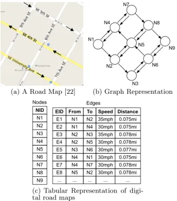
Traditional routing systems utilize digital road maps [23, 36, 38, 47]. Figure 2(a) shows a physical road map and Fig-ure 2(b) shows its digital, i.e., graph-based, representation. Road intersections are often modeled as vertices and the road segments connecting adjacent intersections are repre-sented as edges in the graph. For example, the intersec-tion of ‘SE 5th Ave’ and ‘SE University Ave’ is modeled as node N1. The segment of ‘SE 5th Ave’ between ‘SE Uni-versity Ave’ and ‘SE 4th Street’ is represented by the edge N1-N4. The directions on the edges indicate the permitted traffic directions on the road segments. Digital roadmaps also include additional attributes for road-intersections (e.g., turn restrictions) and segments (e.g., center-lines, road-classification, speed-limit, historic speed, historic travel time, address-ranges, etc.) Figure 2(c) shows a tabular represen-tation of the digital road map. Additional attributes are shown in the node and edge tables respectively. For exam-ple, the entry for edge E1 (N1-N2) in the edges table shows its speed and distance. Such datasets include roughly 100 million (108_{) edges for the roads in the U.S.A. [36]}

Route determination services [33,49], abbreviated as rout-ing services, include the followrout-ing two services [45]. The first deals with determination of a best route given a start location, end location, optional waypoints, and a prefer-ence function. Here, choice of preferprefer-ence function could be: fastest, shortest, easiest, pedestrian, public transportation, avoid locations/areas, avoid highways, avoid tollways, avoid U-turns, and avoid ferries. Route finding is often based on classic shortest path algorithms such as Dijktra’s [28], A* [11], hierarchical [24, 25, 46, 48], materialization [42, 44, 46], and other algorithms for static graphs [4,6–10,17–19,39, 43]. Shortest path finding is often of interest to tourists as well as drivers in unfamiliar areas. In contrast, commuters often know a set of alternative routes between their home and work. They often use an alternate service to compare their favorite routes using real-time traffic information, e.g., scheduled maintenance and current congestion. Both ser-vices return route summary information along with auxiliary details such as route maneuver and advisory information, route geometry, route maps, and turn-by-turn instructions in an audio-visual presentation media.

3. EMERGING SPATIAL BIG DATA

SBD are significantly more detailed than traditional digi-tal roadmaps in terms of attributes and time-resolution. In

this subsection we describe three representative sources of SDB that may be harnessed in next generation routing ser-vices.

Spatio-Temporal Engine Measurement Data: Many mod-ern fleet vehicles include rich instrumentation such as GPS receivers, sensors to periodically measure sub-system prop-erties [26, 27, 32, 35, 51, 52], and auxiliary computing, stor-age and communication devices to log and transfer accu-mulated datasets. Engine measurement datasets may be used to study the impacts of the environment (e.g., elevation changes, weather), vehicles (e.g., weight, engine size, energy-source), traffic management systems (e.g., traffic light tim-ing policies), and driver behaviors (e.g., gentle acceleration or braking) on fuel savings and GHG emissions. These datasets may include a time-series of attributes such as ve-hicle location, fuel levels, veve-hicle speed, odometer values, engine speed in revolutions per minute (RPM), engine load, emissions of greenhouse gases (e.g., CO2 and NOX), etc. Fuel efficiency can be estimated from fuel levels and distance traveled as well as engine idling from engine RPM. These attributes may be compared with geographic contexts such as elevation changes and traffic signal patterns to improve understanding of fuel efficiency and GHG emission. For ex-ample, Figure 3 shows heavy truck fuel consumption as a function of elevation from a recent study at Oak Ridge Na-tional Laboratory [5]. Notice how fuel consumption changes drastically with elevation slope changes. Fleet owners have studied such datasets to fine-tune routes to reduce unnec-essary idling [1, 2]. It is tantalizing to explore the potential of this dataset to help consumers gain similar fuel savings and GHG emission reduction. However, these datasets can grow big. For example, measurements of 10 engine vari-ables, once a minute, over the 100 million US vehicles in existence [16, 50], may have 1014_{data-items per year.}

(a) A Road Map [22] (b) Graph Representation

(c) Tabular Representation of digi-tal road maps

Figure 2: Current representation of road maps as directed graphs with scalar travel time values.

(3)

(a) UPS avoids left-turns to save fuel [31].

(b) Petroleum is dominant energy source for US Transportation [55].

(c) Gap between US petroleum consumption and production is large and growing [3, 12].

Figure 1: Eco-routing supports sustainability and energy independence. (Best in color)

GPS Trace Data: A di↵erent type of data, GPS trajecto-ries, is becoming available for a larger collection of vehicles due to rapid proliferation of cell-phones, in-vehicle naviga-tion devices, and other GPS data-logging devices [20] such as those distributed by insurance companies [57]. Such GPS traces allow indirect estimation of fuel efficiency and GHG emissions via estimation of vehicle-speed, idling and con-gestion. They also make it possible to provide personalized route suggestions to users to reduce fuel consumption and GHG emissions. For example, Figure 4 shows 3 months of GPS trace data from a commuter with each point repre-senting a GPS record taken at 1 minute intervals, 24 hours a day, 7 days a week. As can be seen, 3 alternative com-mute routes are identified between home and work from this dataset. These routes may be compared for engine idling which are represented by darker (red) circles. Assuming the availability of a model to estimate fuel consumption from speed profiles, one may even rank alternative routes for fuel efficiency. In recent years, consumer GPS products [20, 53] are evaluating the potential of this approach. Again, a key hurdle is the dataset size, which can reach 1013 _{items per}

year given constant minute-resolution measurements for all 100 million US vehicles.

Figure 3: Engine measurement data improve under-standing of fuel consumption [5]. (Best in color)

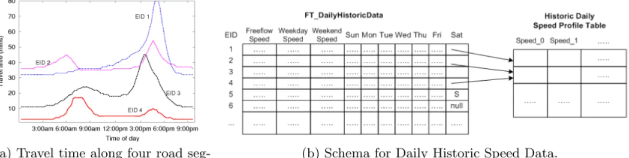
Historical Speed Profiles: Traditionally, digital road maps consisted of center lines and topologies of the road net-works [21, 47]. These maps are used by navigation devices and web applications such as Google Maps [22] to suggest routes to users. New datasets from companies such as NAVTEQ [36], use probe vehicles and highway sensors (e.g., loop de-tectors) to compile travel time information across road seg-ments for all times of the day and week at fine temporal resolutions (seconds or minutes). This data is applied to a profile model, and patterns in the road speeds are identified throughout the day. The profiles have data for every five minutes, which can then be applied to the road segment, building up an accurate picture of speeds based on histor-ical data. Such TD roadmaps contain much more speed information than traditional roadmaps. While traditional

roadmaps (Figure 2(a)) have only one scalar value of speed for a given road segment (e.g., EID 1), TD roadmaps may potentially list speed/travel time for a road segment (e.g., EID 1) for thousands of time points (Figure 5(a)) in a typ-ical week. This allows a commuter to compare alternate start-times in addition to alternative routes. It may even al-low comparison of (start-time, route) combinations to select distinct preferred routes and distinct start-times. For exam-ple, route ranking may di↵er across rush hour and non-rush hour and in general across di↵erent start times. However, TD roadmaps are big and their size may exceed 1013 _items

per year for the 100 million road-segments in the US when associated with per-minute values for speed or travel-time. Thus, industry is using speed-profiles, a lossy compression based on the idea of a typical day of a week, as illustrated in Figure 5(b), where each (road-segment, day of the week) pair is associated with a time-series of speed values for each hour of the day.

Figure 4: A commuter’s GPS tracks over three months reveal preferred routes. (Best viewed in color)

In the near future, values for the travel time of a given edge and start time will be a distribution instead of scalar. For example, analysis of GPS tracks may show that travel-time

(4)

(a) Travel time along four road seg-ments over a day.

(b) Schema for Daily Historic Speed Data.

Figure 5: Spatial Big Data on Historical Speed Profiles. (Best viewed in color)

for a road-segment is not unique, even for a given start-time of a typical week. Instead, it may consist of di↵erent values (e.g., 1, 2, 3 units), with associated frequencies (e.g., 10, 30, 20). The availability of such SBD may allow comparison of routes, start-times and (route, start-time) combinations for statistical distribution criteria such as mean and variance. We also envision richer temporal detail on many preference functions such as fuel cost. Other emerging datasets include those related to pot-holes [40], crime reports [41], and social media reports of events on road networks [56].

4. NEW CHALLENGES

The challenges posed by SBD for state of the art spa-tial computing are significant. First, it requires a change in frame of reference from a snapshot perspective to the per-spective of the individual traveling through a transportation network [14]. For instance, consider the new temporally de-tailed (TD) roadmaps providing historical travel-time (or speed) for each road-segment for every distinct minute of a week. Consider a person sitting in a vehicle and moving along a chosen path in a TD roadmap. She would experi-ence a di↵erent road-segment and its historical speed as well as traversal-time at di↵erent time-intervals, which may be distinct from the start-time.

Second, the growing diversity of SBD significantly increases computational cost because it magnifies the impact of the partial nature and ambiguity of traditional routing query specification. Typically, a routing query is specified by a starting location and a destination. Traditional routing ser-vices would identify a small set of routes based on limited route properties (e.g., travel-distance, travel-time (histori-cal and current)) available in traditional digital roadmap datasets. In contrast, SBD face orders of magnitude richer information, more preference functions (e.g., fuel efficiency, GHG emission, safety, etc.) and correspondingly larger sets of choices.

New questions thus arise in the context of eco-routing: What is the computational structure of determining routes that minimize fuel consumption and GHG emissions? Does this problem satisfy the assumptions behind traditional short-est path algorithms (e.g., stationary ranking of alternative routes assumed by a dynamic programming principle)? For example, temporally detailed roadmaps can potentially pro-vide a distinct route for every possible start-time, even when we just consider travel-time. This raises an optimality chal-lenge of correctly determining the fastest route correspond-ing to each start-time, since rankcorrespond-ing of candidate routes might vary with time of day (rush hour vs. non-rush hour).

It also raises a representation challenge to summarize po-tentially large sets of routes in the result. In addition, the computational challenge of efficiently determining a large collection of routes (e.g., one for each start time and pref-erence function) could perhaps be done by identifying and reducing unnecessary computations via leveraging current cloud computing paradigm (e.g., map reduce) or via novel custom cloud computing paradigms, tentatively called spa-tial cloud computing.

Third, the tremendous diversity of SBD sources substan-tially increases the need for diverse solution methods. For example, methods for determining fuel efficient routes that leverage engine measurement and GPS track datasets may be quite di↵erent from algorithms to identify minimal travel-time routes for a given start-travel-time exploiting TD roadmaps. In addition, SBD data (e.g., TD roadmaps, GPS-tracks and engine-measurement datasets) di↵er in coverage, roadmap attributes and statistical details. For example, TD roadmaps cover an entire country, but provide mean travel-time for a road-segment for a given start-time in a week. In contrast, GPS-track and engine-measurements have smaller coverage to well-travelled routes and time-periods, but may provide a richer statistical distribution of travel-time for each road-segment, perhaps revealing newer patterns such as seasonal-ity. New algorithms are likely to emerge as new SBD become available and as a result, a new, flexible, architecture will be needed to rapidly integrate new datasets and associated al-gorithms.

A fourth challenge area concerns the use of geospatial rea-soning in sensing and inference across space and time. Mul-tiple tradeo↵s (including those arising in privacy considera-tions) can come to the fore with attempts to sense and draw inferences from stable or mobile sensors. New challenges arise from crowd-sourced sensors. For example, the ubiq-uity of mobile phones presents an incredible opportunity for gathering information about all aspects of our world and the people living in it [29]. Already research has shown the po-tential for mobile phones with built-in motion detectors car-ried by everyday users to detect earthquakes mere seconds after they begin [15]. Navigation companies frequently uti-lize mobile phone records to estimate traffic levels on busy highways [56]. How can computers efficiently utilize this prevalent sensing power of mobile phones without drasti-cally impacting battery life or personal privacy concerns? This raises many computer science questions related to sen-sor placement, configuration, etc.

Fifth, we must deal with the many privacy issues sur-rounding geographic information. While location

(5)

informa-tion (GPS in phones and cars) can provide great value to users and industry, streams of such data also introduce “spooky” privacy concerns of stalking and “geo-slavery” [13]. Com-puter science e↵orts at obfuscating location information to date have largely yielded negative results. Thus, many indi-viduals hesitate to engage in mobile commerce due to con-cerns about privacy of their locations, trajectories and other spatio-temporal personal information [30]. Spatio-temporal computing research is needed to address many questions such as: “[should] people reasonably expect that their move-ments will be recorded and aggregated...”? [37]. How do we quantify location privacy in relation to its spatio-temporal precision of measurement? How can users easily understand and set privacy constraints on location information? How does quality of location-based service change with variations in obfuscation level?

Finally, we anticipate that geospatial information will one day be used to make predictions about a broad range of issues including the next location of a car driver, the risk of forthcoming famine or cholera, or the future path of a hurricane. Models may also predict the location of proba-ble tumor growth in a human body or the spread of cracks in silicon wafers, aircraft wings, and highway bridges. Such predictions would challenge the best of machine learning and reasoning algorithms, including directions with geospatial time series data. Many current techniques assume indepen-dence between observations and stationarity of phenomena. Novel techniques accounting for spatial auto-correlation and non-stationarity may enable more accurate predictions. The challenge will be ensuring that such techniques retain com-putational efficiency.

5. ACKNOWLEDGEMENTS

We would like to thank Eric Horvitz (Microsoft), the Com-puting Community Consortium (CCC), Hillol Kargupta (UMBC), Erik Hoel (ESRI), Oak Ridge National Labs (ORNL), Joe Newell and the US-DoD for their helpful comments and sup-port.

6. REFERENCES

[1] American Transportation Research Institute (ATRI). Atri and fhwa release bottleneck analysis of 100 freight significant highway locations.http://goo.gl/C0NuD, 2010.

[2] American Transportation Research Institute (ATRI). Fpm congestion monitoring at 250 freight significant highway location: Final results of the 2010

performance assessment.http://goo.gl/3cAjr, 2010. [3] Austin Brown. Transportation Energy Futures:

Addressing Key Gaps and Providing Tools for Decision Makers. Technical report, National Renewable Energy Laboratory, 2011.

[4] J. Booth, P. Sistla, O. Wolfson, and I.F. Cruz. A data model for trip planning in multimodal transportation systems. InProceedings of the 12th International Conference on Extending Database Technology: Advances in Database Technology, pages 994–1005. ACM, 2009.

[5] G. Capps, O. Franzese, B. Knee, MB Lascurain, and P. Otaduy. Class-8 heavy truck duty cycle project final report.ORNL/TM-2008/122, 2008.

[6] E. Chan and J. Zhang. Efficient evaluation of static and dynamic optimal route queries.Advances in Spatial and Temporal Databases, pages 386–391, 2009. Springer. LNCS 5644.

[7] Edward P.F. Chan and Yaya Yang. Shortest path tree computation in dynamic graphs.IEEE Transactions on Computers, 58:541–557, 2009.

[8] E.P. Chan and H. Lim. Optimization and evaluation of shortest path queries.The VLDB Journal ˜NThe International Journal on Very Large Data Bases, 16(3):343–369, 2007. Springer-Verlag New York, Inc. [9] E.P.F. Chan and N. Zhang. Finding shortest paths in

large network systems. InProceedings of the 9th ACM international symposium on Advances in geographic information systems, pages 160–166. ACM, 2001. [10] T.S. Chang. Best routes selection in international

intermodal networks.Computers & operations research, 35(9):2877–2891, 2008. Elsevier. [11] T. H. Cormen, C. E. Leiserson, R. L. Rivest, and

C. Stein.Introduction to Algorithms. MIT Press, 2001. [12] Davis, S.C. and Diegel, S.W. and Boundy, R.G.

Transportation energy data book: Edition 28. Technical report, Oak Ridge National Laboratory, 2010.

[13] J.E. Dobson and P.F. Fisher. Geoslavery.Technology and Society Magazine, IEEE, 22(1):47–52, 2003. [14] M.R. Evans, K.S. Yang, J.M. Kang, and S. Shekhar. A

lagrangian approach for storage of spatio-temporal network datasets: a summary of results. In Proceedings of the 18th SIGSPATIAL International Conference on Advances in Geographic Information Systems, pages 212–221. ACM, 2010.

[15] M. Faulkner, M. Olson, R. Chandy, J. Krause, K.M. Chandy, and A. Krause. The next big one: Detecting earthquakes and other rare events from

community-based sensors. InInformation Processing in Sensor Networks (IPSN), 2011 10th International Conference on, pages 13–24. IEEE, 2011.

[16] Federal Highway Administration. Highway Statistics. HM-63, HM-64, 2008.

[17] D. Frigioni, M. Io↵reda, U. Nanni, and G. Pasqualone. Experimental analysis of dynamic algorithms for the single.Journal of Experimental Algorithmics (JEA), 3:5, 1998. ACM.

[18] D. Frigioni, A. Marchetti-Spaccamela, and U. Nanni. Fully dynamic algorithms for maintaining shortest paths trees.Journal of Algorithms, 34(2):251–281, 2000. Elsevier.

[19] Daniele Frigioni, Alberto Marchetti-Spaccamela, and Umberto Nanni. Semidynamic algorithms for maintaining single-source shortest path trees. Algorithmica, 22(3):250–274, 1998.

[20] Garmin.http://www.garmin.com/us/.

[21] Betsy George and Shashi Shekhar. Road maps, digital. InEncyclopedia of GIS, pages 967–972. Springer, 2008. [22] Google Maps.http://maps.google.com.

[23] Erik G. Hoel, Wee-Liang Heng, and Dale Honeycutt. High performance multimodal networks. InAdvances in Spatial and Temporal Databases, pages 308–327, 2005. Springer. LNCS 3633.

(6)

Heuristic techniques for accelerating hierarchical routing on road networks.IEEE Transactions on Intelligent Transportation Systems, 3(4):301–309, 2002.

[25] Ning Jing, Yun-Wu Huang, and Elke A.

Rundensteiner. Hierarchical optimization of optimal path finding for transportation applications. In Proceedings of the fifth international conference on Information and knowledge management (CIKM), pages 261–268, 1996. ACM.

[26] H. Kargupta, J. Gama, and W. Fan. The next generation of transportation systems, greenhouse emissions, and data mining. InProceedings of the 16th ACM SIGKDD international conference on Knowledge discovery and data mining, pages 1209–1212. ACM, 2010.

[27] H. Kargupta, V. Puttagunta, M. Klein, and K. Sarkar. On-board vehicle data stream monitoring using minefleet and fast resource constrained monitoring of correlation matrices.New Generation Computing, 25(1):5–32, 2006. Springer.

[28] Jon Kleinberg and Eva Tardos.Algorithm Design. Pearson Education, 2009.

[29] A. Krause, E. Horvitz, A. Kansal, and F. Zhao. Toward community sensing. InProceedings of the 7th international conference on Information processing in sensor networks, pages 481–492. IEEE Computer Society, 2008.

[30] J. Krumm. A survey of computational location privacy.Personal and Ubiquitous Computing, 13(6):391–399, 2009.

[31] Joel Lovell. Left-hand-turn elimination.

http://goo.gl/3bkPb, December 9, 2007. New York Times.

[32] Lynx GIS.http://www.lynxgis.com/. [33] M. Mabrouk, T. Bychowski, H. Niedzwiadek,

Y. Bishr, JF Gaillet, N. Crisp, W. Wilbrink, M. Horhammer, G. Roy, and S. Margoulis. Opengis location services (openls): Core services.OGC Implementation Specification, 5:016, 2005. Citeseer. [34] J. Manyika et al. Big data: The next frontier for

innovation, competition and productivity.McKinsey Global Institute, May, 2011.

[35] MasterNaut. Green Solutions.

http://www.masternaut.co.uk/carbon-calculator/. [36] NAVTEQ.www.navteq.com.

[37] New York Times. Justices Say GPS Tracker Violated Privacy Rights.

http://www.nytimes.com/2012/01/24/us/

police-use-of-gps-is-ruled-unconstitutional. html, 2011.

[38] OpenStreetMap.http://www.openstreetmap.org/. [39] Michalis Potamias, Francesco Bonchi, Carlos Castillo,

and Aristides Gionis. Fast shortest path distance estimation in large networks. InProceedings of the 18th ACM conference on Information and knowledge management, CIKM ’09, pages 867–876, 2009.

[40] Pothole Info. Citizen pothole reporting via phone apps take o↵, but can street maintenance departments keep up? http://goo.gl/cGl3B, 2011.

[41] SafeRoadMaps. Envisioning Safer Roads.

http://saferoadmaps.org/.

[42] Hanan Samet, Jagan Sankaranarayanan, and Houman Alborzi. Scalable network distance browsing in spatial databases. InProceedings of the 2008 ACM SIGMOD international conference on Management of data, SIGMOD ’08, pages 43–54, 2008.

[43] P. Sanders and D. Schultes. Engineering fast route planning algorithms. InProceedings of the 6th international conference on Experimental algorithms, pages 23–36. Springer-Verlag, 2007.

[44] J. Sankaranarayanan and H. Samet. Query processing using distance oracles for spatial networks.Knowledge and Data Engineering, IEEE Transactions on, 22(8):1158–1175, 2010. IEEE.

[45] J.H. Schiller and A. Voisard.Location-based services. Morgan Kaufmann, 2004.

[46] S. Shekhar, A. Fetterer, and B. Goyal. Materialization trade-o↵s in hierarchical shortest path algorithms. In Advances in Spatial Databases, pages 94–111. Springer, 1997.

[47] S. Shekhar and H. Xiong.Encyclopedia of GIS. Springer Publishing Company, Incorporated, 2007. [48] Shashi Shekhar, Ashim Kohli, and Mark Coyle. Path

computation algorithms for advanced traveller information system (atis). InProceedings of the Ninth International Conference on Data Engineering, April 19-23, 1993, Vienna, Austria, pages 31–39. IEEE Computer Society, 1993.

[49] Shashi Shekhar, Ranga Raju Vatsavai, Xiaobin Ma, and Jin Soung Yoo. Navigation systems: A spatial database perspective. InLocation-Based Services, pages 41–82. Morgan Kaufmann, 2004.

[50] Daniel. Sperling and D. Gordon.Two billion cars. Oxford University Press, 2009.

[51] TeleNav.http://www.telenav.com/. [52] TeloGIS.http://www.telogis.com/. [53] TomTom. TomTom GPS Navigation.

http://www.tomtom.com/, 2011.

[54] US Congress. Energy independence and security act of 2007.Public Law, (110-140), 2007.

http://goo.gl/6Kspz.

[55] U.S. Energy Information Adminstration. Monthly Energy Review June 2011.

http://www.eia.gov/totalenergy/data/monthly/. [56] Waze Mobile.http://www.waze.com/.

[57] Wikipedia. Usage-based insurance — wikipedia, the free encyclopedia.http://goo.gl/NqJE5, 2011. [Online; accessed 15-December-2011].

Spatial Big-Data Challenges Intersecting Mobility and Cloud Computing