| 1
Supporting Information
Kinetics of Anionic Living Copolymerization of Isoprene and Styrene using
in situ
NIR
spectroscopy: Temperature Effects on Monomer Sequence and Morphology
Marvin Steube,1, ‡ Tobias Johann,1,‡ Martina Plank,2 Stefanie Tjaberings,3 André H. Gröschel, 3 Markus Gallei,4 Holger Frey,1 and Axel H.E. Müller *,1
1 Institute of Organic Chemistry, Johannes Gutenberg University, Duesbergweg 10-14, 55128 Mainz, Germany
2 Macromolecular Chemistry Department, Technische Universität Darmstadt, Alarich-Weiss Str. 4, 64287 Darmstadt, Germany 3Physical Chemistry, University of Duisburg-Essen, Carl-Benz-Str. 199, 47057 Duisburg, Germany
4 Chair in Polymer Chemistry, Saarland University, 66123 Saarbrücken, Germany
‡ The first two authors (M. Steube, T. Johann) contributed equally.
Table of Contents
1. Materials and Experimental Procedures 2
2. Instrumentation 4
3. Selection of a suitable measurement method for real-time probing of living carbanionic polymerizations 7 4. Linear equation system for the determination of the conversion of the individual monomers 9 5. Theoretical background of the influence of temperature on the preparation of
P(I-co-S) copolymers 10
6. Determination of kSS and kII from homopolymerization kinetics 11
6.1. NMR spectroscopic characterization of polyisoprene and polystyrene 13
6.2. Kinetics of the Synthesis of a (PI-b-PS)2 Tetrablock monitored via real-time NIR probing 18
7. Copolymerization kinetics 19
7.1. Determination of reactivity ratios 21
8. Temperature dependence of reactivity ratios 32
9. Kinetic Monte Carlo simulations 34
10. Microstructure of copolymers 36
11. Monitoring decablock synthesis via NIR real-time probing 39
12. Kinetics and microstructure in the copolymerization in presence of THF 40
13. Microstructural Investigations via NMR on the tapered diblock copolymers 42
14. Thermal properties via DSC measurements 53
15. Copolymer morphologies 55
16. References 59
| 2
1.
Materials and Experimental Procedures
All chemicals and solvents were purchased from Acros Organics Co., Carl Roth GmbH and Sigma-Aldrich Co.
Purification of the Materials
Prior to the use of isoprene and styrene, the monomers were filtered through a column containing basic aluminium oxide to remove stabilizer. Afterwards the targeted monomer volumes of isoprene and styrene were transferred into a flask, dried for 2 days at room temperature over finely ground CaH2, degassed by three cycles of freeze-pump-thaw and distilled (1 · 10−3 mbar) into a flask containing trioctylaluminum obtained by evaporation of solvent from a trioctylaluminium solution under reduced pressure. After stirring at room temperature overnight, the monomers were degassed by one cycle of freeze-pump-thaw and distilled into a graduated ampoule. The combined monomer volume was determined by the graduation and typically showed a loss 1.5 %vol in respect to the targeted value. This can be explained by the loss of monomer during destillation (autopolymerization of the monomers) as well as volume contraction caused by the miscibility.
Cyclohexane was dried over sodium with benzophenone as an indicator under reflux in an argon atmosphere. The dried cyclohexane was distilled into a Mortom flask glass reactor equipped with a rare earth magnetic stirring bar under normal pressure, as described in a previous work.1
THF was dried over diphenylethylenyllithium. For this purpose, a molar ratio of sec-BuLi to diphenyl-ethylene of 1 : 1.2 was used to prevent the presence of sec-BuLi, which is known to undergo side reactions with THF at room temperature. An excess of dry THF was distilled into a graduated ampoule under reduced pressure and the required amount was added by using the graduated flask.
The NIR probe was introduced via an additional glass joint (Fig. S1). The reactor was flushed with argon, the required amount of sec-BuLi solution was added and the polymerization started via the addition of the desired amount of monomer or monomer mixture.
Synthesis of homopolymers PI, PS and block copolymers (PI-
b
-PS)
nRemoval of the stabilizer and drying of the monomers was carried out in separate flasks (see Purification of the Materials). The graduated ampoules containing the dried monomers were attached to the Mortom flask glass reactor. The homopolymerization of styrene or isoprene was started via the addition of the desired amount of monomer. The temperature of the reaction flask was controlled by an external, stirred water bath containing an electronic temperature sensor. The monomer addition of isoprene or styrene was repeated several times, to obtain the desired polymer architecture.
| 3
Synthesis of tapered di- and multiblock copolymers P(I-
co
-S)
nRemoval of the stabilizers was carried out in separated flasks (see Purification of the Materials). The drying of the monomers was carried out in one flask to reduce the number of distillation steps. The addition of the monomer mixture was repeated several times (via a graduated ampoule, see prior section) until the desired number of blocks was achieved.
Synthesis of copolymers with THF addition
Removal of the stabilizer was carried out in separate flasks (see Purification of the Materials). The drying of the monomers was carried out in one flask to reduce the number of distillation steps. A modified procedure was used for this experiment. As the first step, the required amount of dry THF was added to the cyclohexane containing reactor via a graduated ampoule, followed by a measurement of the background spectrum. Subsequently the monomer mixture was added, followed by initiation via sec-BuLi solution. 100 equivalents of THF were used with respect to the active chain ends. The temperature of the reaction flask was controlled by an external, stirred water bath containing an electronic temperature sensor
Termination and work-up
Isopropyl alcohol was degassed by three cycles of freeze-pump-thaw prior to use. The living chain ends were terminated by adding degassed isopropyl alcohol via syringe. To precipitate the polymer, the mixture was poured into an 8-fold volume excess of 50%vol mixture of isopropyl alcohol and methanol, dried at reduced pressure and stored at –20 °C in the absence of light. The pure, colorless polymer was obtained in a quantitative yield.
| 4
Figure S1. A solution of living polystyryllithium in the glass reactor that was used for NIR probing. The NIR probe (left) was introduced via a glass joint. The small Teflon stopper (right) was used to add initiator while flushing the reaction system with Argon 5.0. The large Teflon stopper (middle) was used for multiple monomer additions and as a connection to the Schlenk line.
2.
Instrumentation
Reaction Monitoring via NIR Spectroscopy
Near infrared spectra were recorded on a Nicolet Magna 560 FT-IR spectrometer using the Omnic 7.4
Thermo Scientific software suite on a PbS detector and a CaF2 beam splitter. The IR laser source was
employed as light source, with an aperture of 88, mirror speed of 0.6329 and internal ADC amplification of 8. Data interval was set to 1.928 cm-1 with an internal resolution of 4. Up to 32 scans per spectrum were recorded, depending on measurement time. The NIR probe was connected via glass fibers. All spectra were recorded in the range of 5900 to 6250 cm-1. A background spectrum was measured at the same conditions with at least 64 scans before every experiment series. After the experiment, each individual spectrum was exported to the corresponding binary file, imported to MATLAB and processed as described in the manuscript.
| 5
NMR Spectroscopy
NMR spectra were recorded on a Bruker Avance III 600 spectrometer at 600 MHz (1H-NMR) or 151 MHz (13C-NMR) using a 5 mm TCI-cryo probe with z-gradient and ATM. Signals are referenced internally to residual proton signals of the deuterated solvent.
Peaks of residual solvents are assigned with the respective chemical sum formula and crossed out with a diagonal line.2 Proton Peaks are assigned to the structure pictured in the respective spectrum, and the assignment is given in small letters. Capital Letters are used for the respective carbon atoms. Consequently, the 1H-13C coupling signals are assigned by using a small letter for the proton and a capital letter for the carbon atom. For example, the coupling between the protons a and the carbon B is expressed as a/B.
Standard Size Exclusion Chromatography (SEC)
SEC measurements were performed with THF as the mobile phase (flow rate 1 mL min-1) on an SDV column set from PSS (SDV 103, SDV 105, SDV 106) at 30 °C. Polymer concentrations with a maximum of 1 mg/mL turned out to be suitable to prevent concentration effects.
As indicated, calibration was carried out using polystyrene and 1,4-polyisoprene standards from PSS Polymer Standard Service, Mainz.
Copolymers were evaluated by using the different response factors of the RI (fPI(RI) = 0.0287; fPS(RI) = 0.0391) and the UV-detector (275 nm) (fPI(UV) = 0.0005; fPS(UV) = 0.1226) for 1,4-polyisoprene and polystyrene. Response factors were determined by injecting polystyrene and 1,4-polyisoprene standards at a known concentration onto the column.
The software PSS WinGPC UniChrom (V 8.31, Build 8417) was used to calculate the polyisoprene and polystyrene weight fraction and interpolate the calibration curves of the homopolymer standards to obtain the molecular weight of the copolymer.3
SEC Traces and Polymer Composition
While the evaluation of kinetic and spectroscopic data is usually attributed to the respective repeating units (molar fraction), bulk morphologies depend on the volume fraction of each block.
The conversion diagram (see for example Fig. S9)) depicts the instantaneous styrene incorporation (FS) versus the total conversion during the polymerization. To yield the volume related diagram (volume of instantaneous styrene incorporation (Fv,S) vs. polymer volume fraction) both axes need to be weighted by
the molecular weight and the density of the repeating unit, which was described in detail in the Supporting Information of a previous work.1 The volume fractions of the repeating units are based on the published
| 6 homopolymer densities at 140 °C (ρPI = 0.830 g/cm3, ρPS = 0.969 g/cm3).4 In general a higher molar fraction of polyisoprene units is necessary for a comparable volume of polystyrene repeating units.
Differential Scanning Calorimeter (DSC)
Films were prepared with a thickness of approximately 0.2 mm, obtained by slow evaporation from a chloroform solution, followed by full removal of the solvent under reduced pressure. The thermal properties of the tapered diblock copolymer films were studied with a PerkinElmer DSC 8500 differential scanning calorimeter (DSC) calibrated by n-decane and indium standards. Two heating and one cooling cycle were performed at a rate of 20 K/min in a temperature range between -80 and 130 °C and the glass temperatures were extracted from the second heating cycle. The scans were corrected using a multi-point baseline to remove drifting of the heat flow and normalized by the sample mass.
Transmission electron microscopy (TEM)
Films were prepared with a thickness of around 0.2 mm, obtained by slow evaporation from a chloroform solution followed by a full removal of the solvent under reduced pressure. Samples synthesized at 80° C were thermally annealed for 4 h at 120 °C under nitrogen atmosphere. For characterization of the tapered block copolymer morphology in the bulk state, the films were microtomed from surface to surface at -80 °C into thin slices of 50-70 nm thickness. The collected ultrathin sections were subsequently stained with osmium tetroxide (OsO4) for selective staining of the PI domains, followed by investigation by TEM measurements.
TEM experiments were carried out using a Zeiss EM 10 CR (60kV)/ Olympus Megaview II / ITEM Software build 1276 and a EM 10 electron microscope (Oberkochen, Germany) operating at 60 kV with a slow-scan CCD camera obtained from TRS (Tröndle, Morrenweis, Germany) in bright field mode. The camera was computer-aided using the ImageSP software from TRS.
Transmission Electron Tomography (ET). ET measurements were conducted on a JEOL 2200FS instrument,
operating at an accelerating voltage of 200 kV. The TEM grid was cut in half with a razor blade to fit into the TEM tomography holder. Images were taken with an 2k x 2k Ultra-Scan 1000XP CCD camera (Gatan). Images and Supporting Video S1 were processed with tomviz.org reconstruction software5 using weighted back projection. Volumetric graphics and Supporting Video S2 were compiled with the UCSF Chimera package6 and low-pass filtered with Chimera’s Gaussian filter with 1.5 voxel radius.
| 7
3.
Selection of a suitable measurement method for real-time probing of living
carbanionic polymerization
Since 2010 our group has been investigating the copolymerization kinetics via online 1H-NMR spectroscopy.7,8 This method commonly features excellent distinction of the monomer signals and thus is the method of choice for initial evaluation of reactivity ratios. Typically a good correlation between the polymer microstructure (reactivity ratios) and the resulting physical properties is observed.1,9–11 As computing power as well as other in situ spectroscopic methods have been technically improved, an evaluation of kinetic data can be pursued without the need for sampling. In contrast, more traditional methods like stop-flow or capillary flow techniques have rarely been used over the last years and can be considered as superseded.12 In contrast to the many benefits of NMR spectroscopy, time resolution is limited and typically the polymerization conditions must be tailored to be performed within an NMR tube (use of deuterated solvent, adjusted initiator and monomer concentrations, preparation in glove box). Hence, we found NMR spectroscopy to be unsuitable for the investigation of temperature dependent kinetic measurements like in this work which is attributed to the following main reasons:
(i) Typical reaction times for the homo- and copolymerization of styrene and isoprene are in the range of several hours for [BuLi]0 = 1.5 mmol/L at 40 °C.1 By using typical activation energies,13 reaction times vary in the order of days for T = 10 °C to a few minutes for T = 60 °C, which is not applicable for NMR kinetic investigations. The fast reaction at high temperatures would not yield a sufficient time resolution due to the slow measurement process of NMR spectroscopy (typically not more than one measurement per minute) (Table S1). Additionally, the initial set-up of an NMR measurement can require up to 5 minutes due to the shimming of the magnetic field. To obtain quantitatively reliable results the measurement time must be adjusted to the relaxation time of the protons of interests.
(ii) Also, the NMR tube used as a reaction vessel (typically 1 mL solution with up to 20 weight percent of polymer) prohibits the subsequent investigation of material properties. (iii) In addition, the synthesis of high molecular weight polymers cannot be realized due to difficulties in initiator dosing by targeting an initiator concentration in the range of 10-3 mol/L (≈ 10-6 mol in respect to the total volume of a common NMR tube). Hence, this desired degree of polymerization (𝐷𝑃n) leads to problems with the dosage of the initiator and no reliable rate constants, which are governed by the initiator concentration. The dilution of the initiator by preparing a stock solution also seems questionable in terms of the high reactivity of butyllithium and irreversible termination, which has been stated as a problem in several works.14,15
| 8
Table S1. Comparison of in situ spectroscopic methods for the real-time reaction monitoring of styrene and isoprene.
Method physical foundation setup costs in-situ time
resolution
data evaluationb
NMR nuclear induction & relaxation
extremely difficult
extreme (no) – NMR tube only ~ 1 min Easy, distinct signals
UV-Vis electronic interactions easy cheap (yes) via optical-fiber < 0.1 sa only polymer chain
ends near-IR overtone & combination
molecular vibrations
easy cheap (yes) via optical-fiber < 0.1 s Difficult – overlap of bands mid-IR fundamental molecular
vibrations
difficult high (yes) via crystalline / hollow waveguides
< 0.1 s Easy, distinct signals
a) Monochromator-based systems typically require up to 1 minute, however recent technical developments using digital micromirror devices overcome this issue and enable multiple wavelength measurements within extreme short times.
b) Data evaluation is highly dependent on the molecular structure of the employed monomers. The ratings are given for the case of isoprene/styrene copolymerization.
Besides NMR spectroscopy UV-vis,13,16,17near-IR,18–23 and mid-IR13,24,25 spectroscopies have been applied for real-time reaction monitoring (Table S1). UV-Vis has been established to monitor the strongly colored polystyryllithium chain end, but it is not suitable for detection of monomer concentrations due to the absence of suitable monomer absorbance bands.13 Mid-infrared (mid-IR) spectroscopy has been proven to solve the issues in time-resolution and initiator dosing by enabling the monitoring of the individual monomer consumption in the reaction flask rather to an NMR tube. Also, the time resolution is greatly increased by the Fourier transformation method (FT-IR) compared to dispersive measurements. Unfortunately, the implementation of mid-IR spectroscopy is technically challenging because the optical fibers require crystalline media, e.g. AgCl, or hollow waveguides resulting in mechanically less robust and expensive fibers, which require permanent installation in a polymerization setup.26 In contrast, near -infrared (NIR) spectroscopy utilizes a smaller wavelength for measurement, enabling the use of affordable, flexible silicon-based optical fibers. To summarize, NIR combines the measurement speed of IR spectroscopy by using Fourier transformation with the benefits of optical systems. Comparing all methods, NIR spectroscopy combines a facile setup, low cost and a high time resolution.
| 9
4.
Linear equation system for the determination of the individual monomer
conversion
For each NIR spectrum a linear equation system based on equation S1.4 (184 equations, for each data point corresponding to a data interval of 1.9 cm-1) was formed and solved to obtain the individual monomer concentrations. To prevent overfitting mass conservation was applied (conversion of eq. S1.1 to eq. S1.4 by
S1.2 and S1.3), thus the concentration of PI and PS was bound to initial monomer concentrations. Hence the linear equation system is reduced from 4 parameters (cI, cS, cPI and cPS) to only 2 (cI and cS) (Eq. S2.4).
𝐴(𝜈̃) = 𝑐⏟ 𝐼· 𝜀𝐼(𝜈̃) + 𝑐𝑆· 𝜀𝑆(𝜈̃) 𝑚𝑜𝑛𝑜𝑚𝑒𝑟 𝑎𝑏𝑠𝑜𝑟𝑝𝑡𝑖𝑜𝑛 + 𝑐⏟ 𝑃𝐼· 𝜀𝑃𝐼(𝜈̃) + 𝑐𝑃𝑆 · 𝜀𝑃𝑆(𝜈̃) 𝑝𝑜𝑙𝑦𝑚𝑒𝑟 𝑎𝑏𝑠𝑜𝑟𝑝𝑡𝑖𝑜𝑛 (S1.1) 𝑐𝑃𝐼 = 𝑐𝐼,0− 𝑐𝐼 (S1.2) 𝑐𝑃𝑆 = 𝑐𝑆,0− 𝑐𝑆 (S1.3) 𝐴(𝜈̃) − 𝑐𝑆,0· 𝜀𝑃𝑆(𝜈̃) − 𝑐𝐼,0· 𝜀𝑃𝐼(𝜈̃) = 𝑐𝑆· (𝜀𝑆(𝜈̃) − 𝜀𝑃𝑆(𝜈̃)) + 𝑐𝐼· (𝜀𝐼(𝜈̃) − 𝜀𝐼𝑆(𝜈̃)) (S1.4)
Equation S1. The total absorption A is described as the sum of the absorption of the four individual components: styrene (S),
| 10
5.
Theoretical background of the influence of temperature on the preparation of
statistical P(I-
co
-S) copolymers
The polymer microstructure (e.g., regioisomers of polyisoprene, monomer sequence) is highly dependent on the molecular structure of the employed monomers (e.g. ring-substituted styrenes)9,27 and monomer feed ratio. As we have shown in one of our previous works, also the overall initial initiator and monomer concentrations do influence the microstructure.9 Temperature and the accompanying changes in the pressure can be utilized as a further parameter to manipulate the copolymerization behavior without interfering with the closed polymerization system inside the reaction vessel. The polymerization of isoprene and styrene features two unique properties: (i) The disparate reactivity ratios are mainly dependent on the crossover behavior of both monomers, hence reactivity ratios do not adequately represent the copolymerization behavior.9 For sufficient insight, the homo-propagation rate constants, kSS, and kII, and the cross-propagation rate constants, kSI and kIS, must be evaluated. (ii) As shown by Fontanille and coworkers the homopolymerization rate of isoprene, kII, shows a higher activation energy, as compared to the other parameters when performed in aromatic solvents.13 Subtle changes between cyclohexane and the more polarizable benzene as a solvent in the anionic polymerization are commonly known.13,14,28–30 While precise predictions cannot be made, a comparable behavior can be expected for cyclohexane, meaning different temperature dependencies of the individual propagation rate constants. In this way reactivity ratios and the resulting gradient structure of the tapered block copolymer are postulated to be also dependent on the polymerization temperature when performing the copolymerization in cyclohexane.
| 11
6. Determination of
k
SSand
k
IIfrom Homopolymerization Kinetics
Table S2.Determination of homo-propagation rate constants for isoprene and styrene homopolymerization in the temperature range from 10 to 60 °C. The apparent rate constants kapp equal the slope of the logarithmic monomer consumption versus time (Fig. S2 and S3) and were
converted to the effective rate constants accounting for the chain end concentrations (cBuLi1/2 for styrene, cBuLi1/4 for isoprene).
T [°C] [Ini]isoprene [mmol/L] 10-3kII
[(L/mol)0.25·s-1] 10-3𝒌 𝐈𝐈 𝒂𝒑𝒑[𝐦𝐢𝐧−𝟏] [Ini] styrene [mmol/L] 10-3 kSS [(L/mol)0.5·s-1] 10-3𝒌 𝐒𝐒 𝒂𝒑𝒑 [𝐦𝐢𝐧−𝟏] 10 1.17 0.118 1.31 1.57 1.79 4.25 15 1.17 0.276 2.96 1.57 2.87 6.81 20 1.17 0.500 5.53 1.57 4.43 10.5 25 1.17 0.883 9.76 1.57 6.95 16.4 30 1.17 1.47 16.2 1.57 10.9 25.8 35 1.17 2.46 27.1 1.57 16.1 37.9 40 1.17 3.81 41.9 1.57 23.2 54.3 45 1.17 5.25 57.5 1.57 31.0 72.4 50 0.782a 10.1 109 0.753a 65.2 107 60 0.855a 24.2 248 0.816a 140 240
a Although these homo-propagation rate constants were determined on the same batch, initiator concentrations differ due to the increasing dilution caused
by every monomer addition step.
Figure S2. Normalized logarithmic monomer consumption versus time for the isoprene homopolymerization. Values for 10 to
45 °C were extracted from the homopolymerization experiments performed within one batch (Fig. S4-5), 50 °C and 60 °C were extracted from the (PI-b-PS)2 tetrablock synthesis (Fig. S8-9).
Figure S3. Normalized logarithmic monomer consumption versus time for the styrene homopolymerization. Values for 10 to
45 °C were extracted from the homopolymerization experiment performed within one batch (Fig. S4-5), 50 °C and 60 °C were extracted from the (PI-b-PS)2 tetrablock synthesis (Fig. S8-9).
| 12
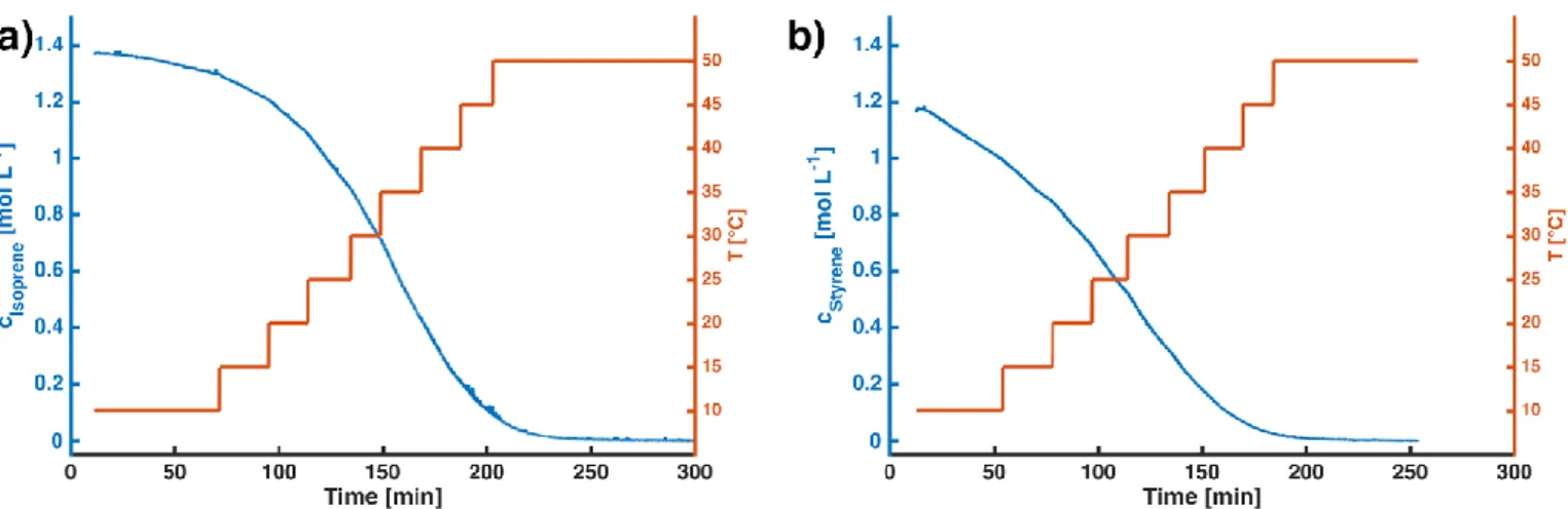
Figure S4. Plot of monomer consumption versus time (blue line) for (a) isoprene homopolymerization and (b) styrene homopolymerization experiments. The red line represents the temperature within the reaction flask, which was gradually increased in steps of 5°C to obtain several temperature dependent rate constants in the range from 10 to 45 °C. Evaluation at 50 °C was not performed due to low monomer content and thus increased measurement noise. Conditions: (a) isoprene homopolymerization: T = 10 to 50°C, cBuLi = 1.17 mmol; (b) styrene homopolymerization: T = 10 to 50 °C, cBuLi = 1.57 mmol.
Figure S5. A) SEC Eluogram (RI detector) of 1,4-polyisoprene (PI) and polystyrene (PS) homopolymer (Solvent: THF, Detector:
RI) used to determine homo-propagation rate constants for PI and PS (Fig. S4). B) Molecular weight distributions after calibration. PS standards were used for calibration for measurement of the PS sample, and well-defined PI standards were used for the PI sample. In this manner, absolute molecular weights have been obtained, showing good agreement with the targeted value of Mn(target) = 80 kg/mol. The deviation of the molecular weight can be attributed to autopolymerization of the monomers during the drying period of three days. This is especially pronounced for styrene and clearly visible by a residue in the flask used for purification after distillation of the monomers.
| 13
6.1 NMR Spectroscopic Characterization of Polyisoprene and Polystyrene
Figure S6A.1H-NMR spectrum (600 MHz, CDCl
3) of polystyrene.
Figure S6B.13C-NMR spectrum (150 MHz, CDCl
3) of polystyrene.
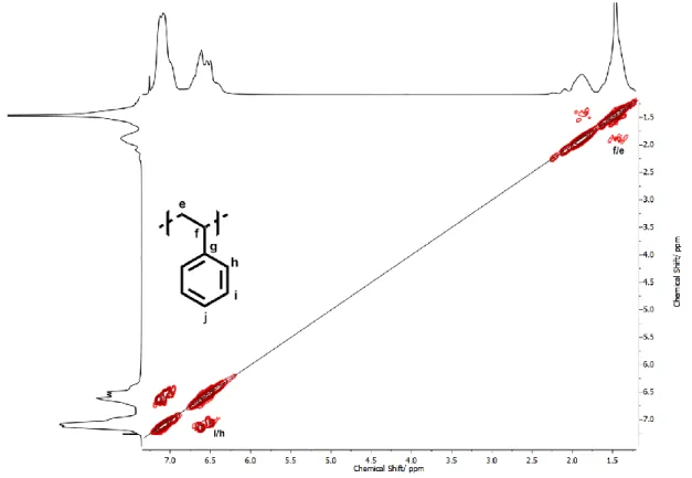
Figure S6C.1H-1H COSY-NMR spectrum (600 MHz, CDCl
| 14
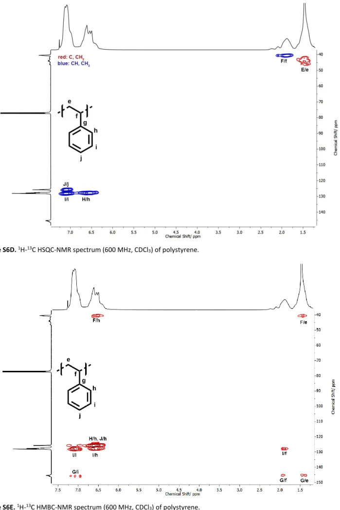
Figure S6D.1H-13C HSQC-NMR spectrum (600 MHz, CDCl
3) of polystyrene.
Figure S6E.1H-13C HMBC-NMR spectrum (600 MHz, CDCl
| 15
Figure S7A.1H-NMR spectrum (600 MHz, CDCl
3) of polystyrene.
Figure S7B.13C-NMR spectrum (150 MHz, CDCl
3) of polyisoprene. The shift of the signals marked with (*) are not visible in the 1H-NMR spectrum and have been assigned via 2D-NMR spectroscopy.
| 16
Figure S7C. 1H-1H COSY-NMR spectrum (600 MHz, CDCl
3) of polyisoprene.
Figure S7D. 1H-13C HSQC-NMR spectrum (600 MHz, CDCl
| 17
Figure S7E. 1H-13C HMBC-NMR spectrum (600 MHz, CDCl
3) of polyisoprene.
The evaluation of the signals in the NMR spectra of polyisoprene is rather complex, due to the presence of different isomers (cis 1,4-PI, trans 1,4-PI, 3,4-PI). Especially in the 13C-NMR spectrum, the formation of different triads consisting of these 3 units, as well as different configurations (head-to-head, tail-to-tail, head-to-tail and the respective inverse configurations) leads to a spectrum rich in signals.
Signals that have been assigned in the spectra always belong to the respective repeating unit (cis 1,4-PI,
trans 1,4-PI, 3,4-PI), surrounded by two (cis or trans) 1,4-PI units, as this is the main unit present in the
investigated polymers. No attention has been drawn to other triads due to the negligible amount of these linkages and the significant overlap of the signals in the 13C NMR spectrum (Δδ ≈ 0.5 ppm). No distinction has been made in the evaluation of the cis and trans signals of the carbons m, n and o due to the minor difference in the chemical shift in 1H and 13C NMR spectra.
Chemical shifts of other triads/diads can be found in the work of Tanaka et. al. for trans and cis 1,4-PI31 and in the work of Gronski et. al.32 and others33–36 for 3,4-PI units.
All signals were assigned via 2D NMR spectroscopy (see Fig. S7C-S7E) and agree with existing literature on this topic.31–36
| 18
6.2 Kinetics of the Synthesis of a (PI-
b
-PS)
2Tetrablock monitored via real-time NIR probing
Figure S8. Plot of monomer consumption (styrene: blue line, isoprene: red line) versus time of the preparation of a sequential
(PI-b-PS)2 tetrablock. The first two blocks were prepared at 60° C, the subsequent next two blocks at 50 °C. The change in volume at each addition was considered for the calculation of the chain end concentration. Conditions: T = 50 °C, isoprene, cBuLi = 0.78 mmol; T= 50 °C, styrene, cBuLi = 0.75 mmol; T= 60 °C, isoprene, cBuLi = 0.86 mmol; T= 50 °C, styrene, cBuLi = 0.82 mmol.
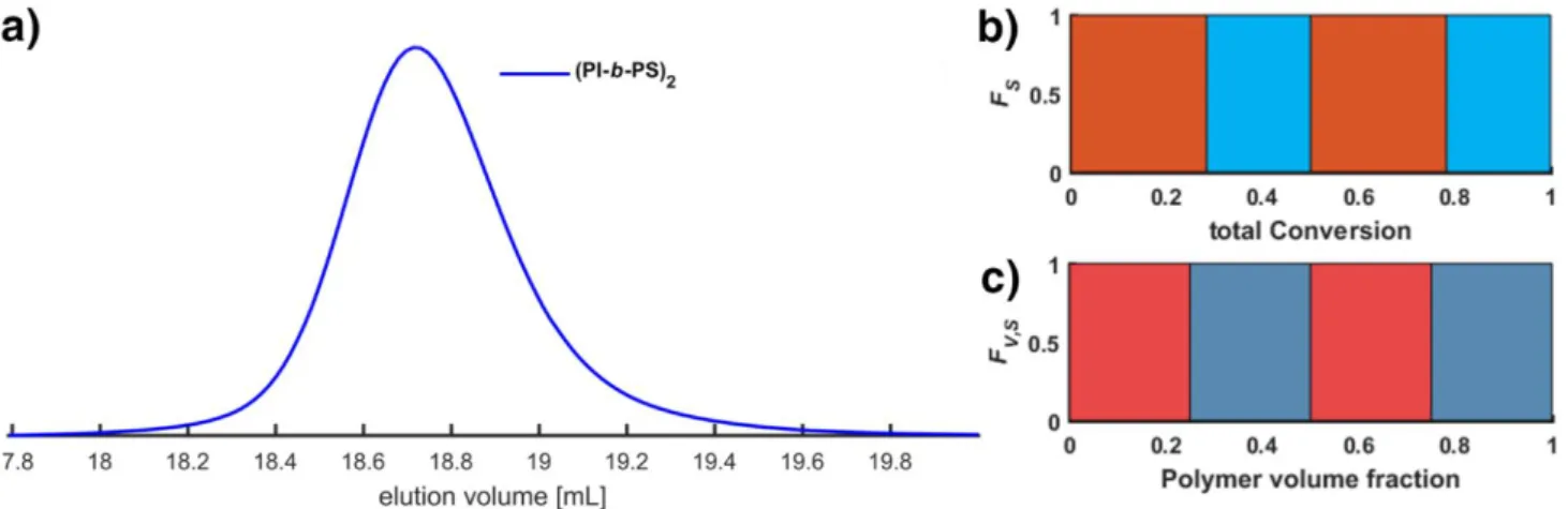
Figure S9. a) SEC Eluogram (RI detector) with Mn and Đ based on dual calibration by using PI and a PS standards according to their weight fraction (see Instrumentation Section; Mn = 154 kg/mol; Đ = 1.10 kg/mol; Mn(target) = 160 kg/mol). b) Composition profile according to molar fraction c) Composition profile according to volume fraction of the sequential diblock copolymer (PI-b-PS)2. A 57 %mol molar fraction of isoprene was used (see diagram b)) to obtain a 50 %vol volume fraction of isoprene (see diagram c)). A lamellar morphology can be expected.
| 19
7. Copolymerization Kinetics
Figure S10. Total combined monomer conversion versus reaction time for each performed copolymerization (10 °C to 60 °C)
| 20
Figure S11. Individual monomer conversion (styrene: blue line, isoprene: red line) versus reaction time for each performed
copolymerization (10 °C to 60 °C). The dashed line shows the simulated time-dependent monomer conversion via KMC based on the experimentally determined rate constants. The deviation of the simulated curves from the experimental data is mainly based on the homo-propagation rate of isoprene. Variation in kII influences the period until the polymerization of styrene proceeds, hence the horizontal shift of the styrene conversion is mainly based on kII. During the copolymerization the homo-propagation of isoprene proceeds in the presence of styrene, and thus the rate constant is slightly altered compared to the values obtained in pure homopolymerization experiments.
| 21
7.1 Determination of Reactivity Ratios
Theoretical Background
The reactivity ratios are defined as the ratio of homopropagation rate versus crossover rate. In the case of the copolymerization of isoprene and styrene chain end aggregation phenomena need to be considered. Equations S2.1 to S2.26 represents the derivation of the rate equations of copolymerization (S2.27-S2.29) that consider the chain end aggregation phenomena. Based on these equations the Mayo-Lewis equation can be derived (S2.30 to S2.32 to yield S2.33). As shown below, the Mayo-Lewis equation shows no dependence on the aggregation behavior, even though the aggregation-based rate equations were used for the derivation. Hence, the exact knowledge of the aggregation type is not necessary for the evaluation of reactivity ratios. Therefore, in this work the determination of the crosspropagation rate constants was performed by determining the reactivity ratios and calculating the rate constants from those. This approach omits solving of the differential equation system, which is numerically difficult due to the exponents of ¼ and ½ in equation S2.27 to S2.29.
The four elemental reactions of copolymerization as proposed by Mayo and Lewis are:
PS−+ S 𝑘SS′ → PS− (S2.1) PI−+ S 𝑘IS ′ → PS− (S2.2) PS−+ I 𝑘SI ′ → PI− (S2.3) PI−+ I 𝑘II′ → PI− (S2.4)
Equations S2.1 to S2.4 can be used to describe the rate of reaction:
−d[S] d𝑡 = 𝑘SS ′ [S][PS−] + 𝑘 IS ′ [S][PI−] (S2.5) −d[I] d𝑡 = 𝑘II ′[I][PI−] + 𝑘 SI′ [I][PS−] (S2.6) −d[PS −] d𝑡 = d[PI−] d𝑡 = 𝑘SI ′ [I][PS−] − 𝑘 IS′ [S][PI−] (S2.7)
| 22
4PI−→←PI4− (S2.8)
2PS−→
←PS2− (S2.9)
These reactions S2.8 and S2.9 can be described with the following equilibria:
𝐾PI,agg= [PI4−] [PI−]4 (S2.10) 𝐾PS,agg= [PS2−] [PS−]2 (S2.11)
Experimentally only the individual concentrations of the aggregated and non-aggregated chain ends are not accessible, hence the total anion concentration per species (PS or PI) is suitable to describe this dependence:
[PI−]
total= [PI−] + 4[PI4−] (S2.12)
[PS−]
total= [PS−] + 2[PS2−] (S2.13)
The combination of equation S2.12 and S2.13 with S2.10 and S2.11 respectively yields the expression of the non-aggregated chain end concentration:
[PI−] = ([PI4−] 𝐾PI,agg ) 1 4 = ( 1
4([PI−]total− [PI−])
𝐾PI,agg ) 1 4 (S2.14) [PS−] = ([PS2 −] 𝐾PS,agg ) 1 2 = ( 1 2([PS−]total− [PS−]) 𝐾PS,agg ) 1 2 (S2.15)
To simplify equation S2.14 and S2.15 the concentration of non-aggregated chain ends are considered negligible compared to the total anion concentration:
[PI−]
total ≫ [PI−] (S2.16)
[PS−]
| 23 Hence, the terms S2.14 and S2.15 are simplified:
[PI−] = ( 1 4([PI−]total) 𝐾PI,agg ) 1 4 = ( 1 4𝐾PI,agg ) 1 4 ([PI−] total) 1 4 (S2.18) [PS−] = ( 1 2([PS−]total) 𝐾PS,agg ) 1 2 = ( 1 2𝐾PS,agg ) 1 2 ([PS−] total) 1 2 (S2.19)
The combination of equation S2.18 and S2.19 with the differential rate equations S2.5-S2.7 yields the rate equations in dependence of the total chain end anion concentration.
−d[S] d𝑡 = 𝑘SS ′ [S] ( 1 2𝐾PS,agg ) 1 2 ([PS−] total) 1 2+ 𝑘IS′ [S] ( 1 4𝐾PI,agg ) 1 4 ([PI−] total) 1 4 (S2.20) −d[I] d𝑡 = 𝑘II ′[I] ( 1 4𝐾PI,agg) 1 4 ([PI−] total) 1 4+ 𝑘SI′ [I] ( 1 2𝐾PS,agg) 1 2 ([PS−] total) 1 2 (S2.21) −d[PS −] d𝑡 = d[PI−] d𝑡 = 𝑘SI′ [I] ( 1 2𝐾PS,agg ) 1 2 ([PS−] total) 1 2− 𝑘IS′ [S] ( 1 4𝐾PI,agg ) 1 4 ([PI−] total) 1 4 (S2.22)
To summarize, the chain end aggregation introduces an additional equilibrium of the non-aggregated and aggregated chain ends. Experimentally, this equilibrium is difficult to be considered; therefore, a common approach is to include the equilibrium constant in the rate constants.
𝑘SS= 𝑘SS′ ( 1 2𝐾PS,agg ) 1 2 (S2.23) 𝑘SI= 𝑘SI′ ( 1 2𝐾PS,agg) 1 2 (S2.24) 𝑘IS= 𝑘IS′ ( 1 4𝐾PI,agg ) 1 4 (S2.25)
| 24 𝑘II= 𝑘II′ ( 1 4𝐾PI,agg ) 1 4 (S2.26)
By combining equations S2.23-S2.26 with the equation S2.20-S2.22 the differential rate equations can be
described by experimentally known values such as the total anion concentration, the monomer concentration and the rate constants that can be obtained via measurements.
−d[S] d𝑡 = 𝑘SS[S]([PS −] total) 1 2+ 𝑘IS[S]([PI−]total) 1 4 (S2.27) −d[I] d𝑡 = 𝑘II[I]([PI −] total) 1 4+ 𝑘SI[I]([PS−]total) 1 2 (S2.28) −d[PS −] d𝑡 = d[PI−] d𝑡 = 𝑘SI[I]([PS −] total) 1 2− 𝑘IS[S]([PI−]total) 1 4 (S2.29)
As described by Mayo and Lewis, the differential rate constants can be used to derive the copolymerization equation. In the first step, equation S2.28 is divided by equation S2.27.
d[I] d[S]= 𝑘II[I]([PI−]total) 1 4+ 𝑘SI[I]([PS−]total) 1 2 𝑘SS[S]([PS−]total) 1 2+ 𝑘IS[S]([PI−]total) 1 4 = [I] [S] 𝑘II([PI−]total) 1 4+ 𝑘SI([PS−]total) 1 2 𝑘SS([PS−]total) 1 2+ 𝑘IS([PI−]total) 1 4 = [I] [S] 𝑘II([PI −] total) 1 4 ([PS−] total) 1 2 + 𝑘SI 𝑘SS+ 𝑘IS([PI −] total) 1 4 ([PS−] total) 1 2 (S2.30)
With the steady state assumption that the number of chain ends is constant and hence no termination is present, the following equation can be described:
𝑘SI[I]([PS−]total) 1 2= 𝑘IS[S]([PI−]total) 1 4 (S2.31) ([PI−] total) 1 4 ([PS−] total) 1 2 = 𝑘SI[I] 𝑘IS[S] (S2.32)
| 25 By combining the steady-state assumption S2.32 with equation S2.30 the Mayo-Lewis equation can be obtained:
d[I] d[S]= [I] [S] 𝑘II𝑘𝑘SI[I] IS[S]+ 𝑘SI 𝑘SS+ 𝑘IS𝑘𝑘SI[I] IS[S] = [I] [S] 𝑘II[I] 𝑘IS[S]+ 1 𝑘SS 𝑘SI + [I] [S] = [I] [S] 𝑟I [I] [S]+ 1 𝑟S+[S][I] = [I] [S] 𝑟I[I] + [S] 𝑟S[S] + [I] (S2.33)
As shown in this derivation of the Mayo-Lewis equation S2.33 the chain end aggregation is not present anymore. Hence, the evaluation of reactivity ratios based on methods that rely on the Mayo-Lewis equation such as the Fineman-Ross, Kelen-Tüdös or Meyer-Lowry formalism is independent of chain end aggregation phenomena. Note that in the following equations used for the determination of reactivity ratios the indices can be exchanged, hence the evaluation can be performed on the basis of 𝑓𝑆 or 𝑓𝐼.
The equation S2.33 can be described using the monomer feed f and the instantaneous monomer incorporation ratio F:
𝐹𝐼=
𝑟I𝑓I2+ 𝑓I𝑓𝑆
𝑟I𝑓𝐼2+ 2𝑓I𝑓𝑆+ 𝑟S𝑓S2
(S2.34)
For the Fineman-Ross formalism, equation S2.34 is linearized:
𝐺 = 𝐻𝑟I− 𝑟S (S2.35) 𝐺 =𝑓I(2𝐹𝐼− 1) (1 − 𝑓I)𝐹𝐼 (S2.36) 𝐻 = 𝑓I 2(1 − 𝐹 𝐼) (1 − 𝑓I)2𝐹𝐼 (S2.37)
The Kelen-Tüdös formalism uses a correction factor α to correct for biases in the Fineman-Ross formalism.
𝜂 = (𝑟I+ 𝑟S 𝛼) 𝜇 − 𝑟S 𝛼 (S2.38) 𝛼 = √𝐻min𝐻max (S2.39) 𝜂 = 𝐺 𝛼 + 𝐻 (S2.40) 𝜇 = 𝐻 𝛼 + 𝐻 (S2.41)
| 26 1 − 𝑋 = [I] + [S] [I]0+ [𝑆]0 = [M] [M]0 = ( 𝑓I 𝑓I,0 ) (1−𝑟𝑟S S) (1 − 𝑓I 1 − 𝑓I,0 ) (1−𝑟𝑟I 𝐼) ( 𝑓I,0−2 − 𝑟1 − 𝑟S 𝐼− 𝑟S 𝑓I−2 − 𝑟1 − 𝑟S 𝐼− 𝑟S ) ((1−𝑟1−𝑟I𝑟S 𝐼)(1−𝑟S)) (S2.42)
In the case of an ideal copolymerization (𝑟I𝑟S= 1) the last term of the Meyer-Lowry equation becomes 0 and the equation can be linearized. This essentially leads to the equation proposed by Jaacks:
ln [I] [I]0= 𝑟Iln
[S]
[S]0 (S2.43)
Method of determination of reactivity ratios
Reactivity ratios were determined from the time-dependent monomer conversions by using the Mayo-Lewis equation (Eq S2.34) the Fineman-Ross formalism (Eq S2.35-S.37), the Kelen-Tüdös formalism (Eq
S2.38-S2.41) and the Meyer-Lowry formalism (Eq S2.42). The calculation of the fraction of S in the copolymer, FS, is extremely prone to numerical errors, especially in case of only small differences within the data points. Thus, for the determination of highly disparate reactivity ratios via differential approaches (Mayo-lewis, Fineman-Ross, Kelen-Tüdös) specialized methods for the calculation of the derivative must be applied. Simple calculation of the derivative via finite-difference methods results in noise amplification. We found the differentiation by using total-variation regularization the method of choice.37 Unfortunately, even with optimized methods for the calculation of F the subtle change in gradient cannot be accurately determined via direct fitting of the Mayo-Lewis, Fineman-Ross or Kelen-Tüdős formalism (FigureS14-S16
and Table S3). Hence for the discussion, only the reactivity ratios determined via Meyer-Lowry are considered.38
| 27
Figure S12. Individual monomer conversion (styrene: blue line, isoprene: red line) versus total monomer conversion for each
performed copolymerization (10 °C to 60 °C). With increasing temperature, the change in slope becomes less sharp, a first indicator for less pronounced gradient of the resulting copolymer microstructure.
| 28
Figure S13. Meyer-Lowry fits (red line) (1-X (total conversion)) versus actual fraction of styrene in the feed, fs) used for the evaluation of the reactivity ratios. In all cases excellent correlation was obtained. Due to this excellent correlation the measurement points (blue dots) are overlaid by the Meyer-Lowry fit.
| 29
Figure S14. Evaluation of reactivity ratios via numerical fitting of the Mayo-Lewis copolymerization equation (red line). The
data points (blue dots) were calculated by using total variable regularization method for the calculation of FS and are prone to numerical noise. Therefore, this method shows increased uncertainty of the determined reactivity ratios and are given for reference only.
| 30
Figure S15. Evaluation of reactivity ratios using the Fineman-Ross formalism (red line). The data points (blue dots) were calculated using the total variable regularization method for the calculation of FS and are prone to numerical noise. Therefore, this method shows increased uncertainty of the determined reactivity ratios and are given for reference only.
| 31
Figure S16. Evaluation of reactivity ratios using the Kelen-Tüdös formalism (red line). The data points (blue dots) were calculated using total variable regularization method for the calculation of FS and are prone to numerical noise. Therefore, this method shows increased uncertainty of the determined reactivity ratios and are given for reference only. The data points are not distributed uniformly in regard of µ. Therefore, discrepancies of the fit to the datapoints are difficult to determine by eye. However, all data points have been used for the linear regression.
| 32
8. Temperature
Dependence of Reactivity Ratios
Table S3. Calculated values for reactivity ratios (see Fig. S17 for illustration).
T [°C] Meyer-Lowry
a Mayo-Lewisb Fineman-Rossb Kelen-Tüdösb
rI rS rI rS rI rS rI rS 10 10.24 0.010 10.17 0.019 10.45 0.012 n.d.c n.d.c 20 10.80 0.013 11.26 0.022 11.17 0.023 10.72 0.016 30 11.15 0.017 10.95 0.016 11.18 0.021 10.92 0.016 40 10.94 0.029 10.27 0.019 10.96 0.035 10.05 0.014 50 9.91 0.033 9.61 0.024 9.76 0.030 9.04 0.016 60 9.93 0.039 10.77 0.041 12.86 0.096 10.54 0.036 80 d 10.03 0.072 n.d. n.d. n.d. n.d. n.d. n.d. THF (25 °C)a 0.61 1.839 n.d.c n.d.c n.d.c n.d.c n.d.c n.d.c
a: Only Meyer-Lowry formalism was suitable for accurate evaluation of the reactivity ratios. b: Given only for reference and the comparison of the different methods
c: Not determined due to high numerical noise induced by the necessary calculation of Fs.
| 33
Figure S17. Comparison of the reactivity ratios in benzene and cyclohexane in dependency of the reaction temperature. Values
in benzene were taken from Fontanille and coworkers.13 Prediction of the reactivity ratios were performed by feeding the Arrhenius equation and calculating the reactivity ratios for every temperature in the rage of 10 to 80 °C. (a) Reactivity ratio of isoprene versus temperature. In benzene the homopolymerization of isoprene is favored at higher temperatures, leading to high rI values. In contrast only a subtle decrease in rI can be seen for isoprene in cyclohexane. (b) Reactivity ratio of styrene versus temperature. rS increases with higher reaction temperature up to 4 fold in the range from 10 to 80 °C. (c) Graph of rI * rS versus temperature to demonstrate the influence of temperature leading to an ideal copolymerization behavior. With increasing temperature, the copolymerization proceeds to show ideal behavior (rS * rI = 1) for both cyclohexane and benzene. (d) Graph of the ratio of rI/rS versus temperature. A high ratio denotes disparate reactivity values, an indicator for the steepness of the gradient. With increasing temperature, a less steep gradient is observed, when the polymerization is performed in cyclohexane. In contrast to the behavior in benzene an increased gradient is expected.
| 34
9. Kinetic Monte Carlo Simulations
The kinetic Monte Carlo simulation model was developed based on the stochastic simulation algorithm by Gillespie.39,40 In this approach the continuum-based reaction rates (e.g. rate constants determined via NIR) are converted to number-based probabilities using the following equations:
𝑘𝑀𝐶II = 𝑘II (N𝑉)1/4 𝑘𝑀𝐶SS = 𝑘SS (N𝑉)1/2 𝑘𝑀𝐶IS= 𝑘IS (N𝑉)1/4 𝑘𝑀𝐶SI= 𝑘SI (N𝑉)1/2
The simulation volume (typically 2·10-16 L) was used to convert the concentration of all reagents to number of molecules (typically 92,800,000 molecules of styrene and 92,800,000 molecules of isoprene) in the kMC simulation. For each simulation, the number of polymer chains were set to 500,000 and the polymerization was performed until a conversion of 99.5 % was reached. For better comparison all polymerizations were simulated with the same conditions (Pn(I) = Pn(S) = 464, cBuLi = 1.5 mmol, target MW = 79933 g·mol-1).
For each simulation step the reaction probability is calculated based on the fraction of the total reaction rate of all components:
𝑃𝑣 =
𝑅𝑉
∑𝑣=1𝑀 𝑅𝑉
Then one reaction is chosen using a uniform distributed random number 𝑟𝑛1 = [0. .1] based on the reaction probabilities: ∑ 𝑃𝑣 µ−1 𝑣=1 < 𝑟𝑛1 < ∑ 𝑃𝑣 µ 𝑣
The necessary reaction step to perform the reaction is calculated using another uniformly distributed number 𝑟𝑛2= [0. .1]: 𝜏 = 1 ∑𝑣=1𝑀 𝑅𝑣 ln ( 1 𝑟𝑛2 )
| 35 After the chosen reaction step has been applied, the calculation is started again, until the number of molecules left in the simulation volume is below the desired threshold, governed by the desired conversion (99.5 %). The resulting data is then used for the prediction of SEC traces, segment length distributions and triads. The segment length is defined as the number of coherent monomers of one type without interruption. Implementation of this model was performed in C code, compiled using MinGW GCC compiler 5.1.
| 36
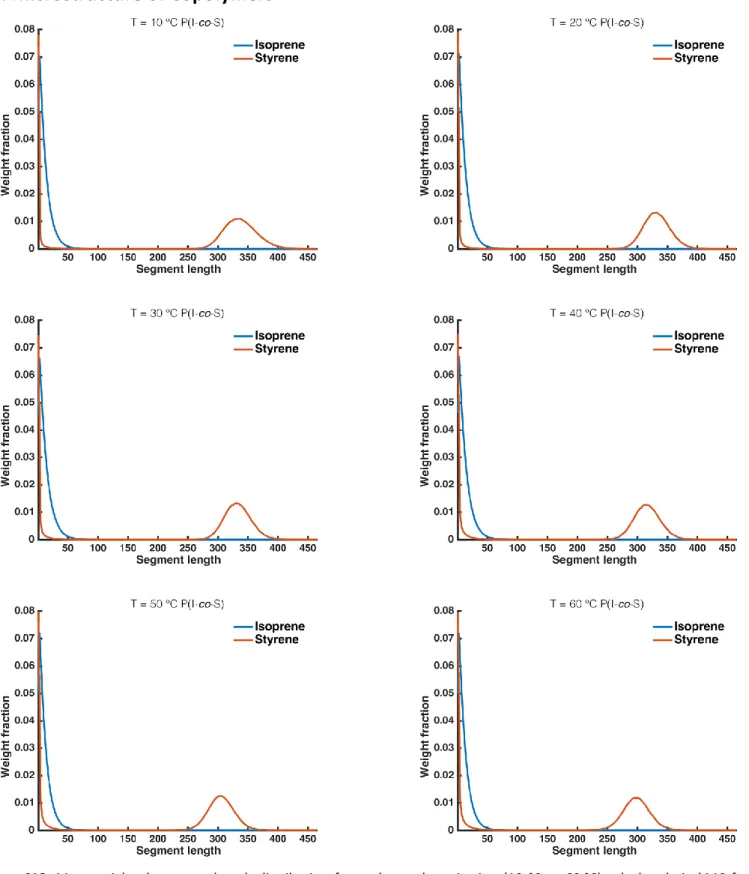
10. Microstructure of Copolymers
Figure S18. Mass weighted segment length distribution for each copolymerization (10 °C to 60 °C) calculated via kMC for isoprene (blue line) and styrene (red line). With increasing temperature, the low molecular weight segments (< 20) for styrene are increased and more styrene is incorporated during the gradient. As a direct result, the size of the styrene block is decreased due to mass conservation.
| 37
Figure S19. Mass weighted molecular weight distribution based on the segment length distribution for each copolymerization
(10 °C to 60°C) calculated via kMC for isoprene (blue line) and styrene (red line). With increasing temperature, the low molecular weight segments (Pn < 20) for styrene are increased and more styrene is incorporated during the gradient. As a direct result the size of the styrene block is decreased due to mass conservation.
| 38
Figure S20: a) Simulated molecular weight distribution (left) of the pure PS block formed during the course of P(I-co-S) copolymerization. b) Simulated low molecular weight segment length distribution (weight based) of PS in P(I-co-S) tapered block copolymers.
Table S4.Analysis of triad distribution and average degrees of polymerization of segments as calculated by kinetic Monte Carlo simulation.
T [°C] T99.5a [h] III/ % IIS + SII / % ISI/ % ISS + SSI / % SIS/ % SSS/ % DPn(I) b DPw(I)b DPn(S)b DPw(S)b DPPeak(S)b 10 48.3 32 15 10 2.2 4.0 37 4,5 11.5 4.4 247 337 20 14.3 32 15 10 2.5 4.0 37 4,4 11.3 4.3 240 332 30 5.4 33 14 9.2 2.9 3.7 38 4,7 12.3 4.6 241 330 40 2.3 32 14 8.7 4.0 3.7 37 4,7 12.1 4.6 218 311 50 0.8 32 15 9.2 4.5 4.1 36 4,4 11.1 4.3 204 306 60 0.4 32 15 8.9 4.9 4.0 36 4,4 11.2 4.3 194 302
a) Predicted reaction time for total monomer conversion of 99.5 %. b) Number-average and weight-average segment lengths of either isoprene or styrene segments respectively. Based on the less steep gradient, induced by higher reaction temperatures, a significant amount of styrene is incorporated into the isoprene rich part during polymerization, leading to smaller sizes of the PS block formed subsequent to formation of the taper. Therefore, the weight average-based segment length Pw decreases drastically. This microstructural change can also be detected in the increasing number of ISS and SSI triads.
| 39
11. Monitoring of decablock copolymer synthesis via NIR real-time probing
Figure S21. a) SEC Eluogram (RI detector) with Mn and Đ based on dual calibration by using PI and a PS standards according to their weight fraction (see Instrumentation Section; Mn = 215 kg/mol; Đ = 1.09; Mn(target) = 240 kg/mol). b) Composition profile according to molar fraction c) Composition profile according to volume fraction of the sequential diblock copolymer P(I-co-S)5. In this case a 50 %mol molar fraction of isoprene was used (see diagram b)) to obtain a volume fraction, resulting in a lamellar morphology as shown in a previous work.1 The lower isoprene content as compared to the sequentially made block copolymers is necessary to obtain a 50 %vol fraction. This can be attributed to the incorporation of polystyrene into the tapered polyisoprene block. This leads to swelling of the tapered polyisoprene block and a shrinkage of the polystyrene block, shifting the gradient towards lower values of the polymer volume fraction. The inflection point of the gradient in the volume diagram (see c)) was used to determine the polymer volume fraction of the block transition. A more detailed description of these tapered multiblock structures is given in a previous work.1
| 40
12. Kinetics and microstructure in the copolymerization in presence of THF
Figure S22. Copolymerization of styrene and isoprene in cyclohexane at 25 °C with addition of 100 equivalents of THF relative
to butyllithium (cBuLi = 1.5 mmol L-1) leading to a copolymer with a strongly deviating monomer sequence as compared to the copolymers prepared in pure cyclohexane. (a) Individual monomer conversions versus time. Due to high temporal resolution (0.33 s per data-point) increased noise is observed. (b) Total monomer conversion versus time after data smoothing. (c) Individual monomer conversion versus total monomer conversion. The slightly favored incorporation of styrene can be seen by the slight curvature of the graph (blue line). (d) Evaluation of the reactivity ratios via Meyer-Lowry formalism. (e) Evaluation of the reactivity ratios via Jaacks method. In this special case an ideal copolymerization (rS·rI = 1) is assumed. (f) Logarithmic representation of the normalized total monomer conversion versus time.
| 41
Figure S23. a) Eluogram (RI detector) with Mn and Đ based on dual calibration by using PI and a PS standards according to their weight fraction (see Instrumentation Section; Mn = 79.9 kg/mol; Đ = 1.09 kg/mol; Mn(target) = 80 kg/mol. b) Composition profile according to molar fraction c) Composition profile according to volume fraction of the copolymer P(I-co-S). In this case a 50 %mol molar fraction of isoprene was used (see diagram b)) resulting in the volume composition visualized in diagram c).
| 42
13. Microstructural Investigations via NMR on the tapered diblock copolymers
1) Poly(isoprene-
co
-styrene)
Figure S24A.1H-NMR spectrum (600 MHz, CDCl
| 43
Figure S24B.13C-NMR spectrum (150 MHz, CDCl3) of Poly(isoprene-co-styrene). The shift of the signals marked with (*) are not visible in the 1H-NMR spectrum of polyisoprene or polystyrene and attributed to different chemical shift of single monomer units attributed to the presence of different triads (TableS4) than III and SSS which are not present in the homopolymers and the block copolymer (PI-b-PS).
The evaluation of the signals in the NMR spectra of polyisoprene homopolymer is known to be rather complex and was discussed in several works. The incorporation of styrene units into the manifold triads of the PI isomers do not allow for an assignment without advanced NMR techniques exceeding the evaluation of 1H and 13C assignments via the 2 dimensional NMR methods as used for PS (Fig. S6) and PI (Fig. S7) homopolymers.
| 44
2) Comparison of homo-, block- and tapered block copolymers
Figure S25A. Stacked 1H-NMR spectra (600 MHz, CDCl
3) of homopolymers (see also Fig. S6 and S7), as well as a block-, and a tapered block copolymer (see also Fig.S25), based on styrene and isoprene.
An assignment of the peaks in the 1H-NMR spectrum can be found in Fig. S6, S7 and S24. We want to emphasize that the block copolymer PI-b-PS is composed of 57 %mol polyisoprene units, while the tapered block copolymer exhibits a 50 %mol fraction of polyisoprene units P(I-co-S).
| 45
Figure S25B. Stacked 13C-NMR spectra (150 MHz, CDCl
3) of homo-, block-, and tapered block copolymers based on styrene and isoprene.
| 46 The selected spectra clearly highlight the differences of block and tapered block copolymers.
The simple architecture of an PI-b-PS block copolymer can be described as two homopolymers linked together. This is visualized by the stacked 1H- and 13C NMR spectra, as the spectrum of PI-b-PS is a simple addition of the signals in the spectra of PI and PS.
In contrast, the spectrum of the tapered block copolymer P(I-co-S) exhibit additional signals which cannot be found in the spectrum of PI, PS or PI-b-PS (for example: 1H-NMR spectrum: 7.6 ppm, 2.75-2.15 ppm). Additionally, the shape of the signals in the overlapping regions (for example: 1H-NMR spectrum: 5.2 - 4.65 ppm, 2.15 – 1.5 ppm) differs for both copolymers. This can be attributed to different chemical surroundings for the PI and PS repeating units. As only III and SSS triads are present in the homopolymers as well in the block copolymer, the tapered block copolymer also shows ISS / SSI, ISI, SII / IIS and SIS monomer sequences, clearly visible in the spectrum of P(I-co-S).
3) Comparison of tapered block copolymers obtained at different polymerization temperatures
Figure S26A. Stacked 1H-NMR spectra (600 MHz, CDCl
3) of tapered block copolymers based on styrene and isoprene obtained by the statistical copolymerization at different polymerization temperatures. The different polymerization temperatures have been assigned in the figure next to the respective spectrum. The spectra do not show a significant difference, confirming a comparable monomer sequence for the copolymerization over the temperature range from 10 to 80 °C.
| 47
Figure S26B. Stacked 1H-NMR spectra (600 MHz, CDCl
3) of tapered P(I-co-S) block copolymers based on styrene and isoprene obtained by the statistical copolymerization at different polymerization temperatures. The different polymerization temperatures have been assigned in the figure next to the respective spectrum and show an increase of the proton resonance signal of the 3,4-units in relation to the proton resonance signal of the 1,4-units. This effect is also known for the respective PI homopolymerization.41
| 48
Figure S26C. Stacked 13C-inverse gated -NMR spectra (600 MHz, CDCl
3) of tapered block copolymers based on styrene and isoprene obtained by the statistical copolymerization at different polymerization temperatures. The different polymerization temperatures have different been assigned in the figure next to the respective spectrum. The spectra do not show a significant difference, confirming the occurrence of similar triades for both tapered block copolymers synthesized at 10 and 80 °C.
| 49
Figure S26D. Stacked 13C-NMR inverse gated spectra (600 MHz, CDCl
3) of tapered block copolymers based on styrene and isoprene obtained by the statistical copolymerization at different polymerization temperatures. The different polymerization temperatures have been assigned in the figure next to the respective spectrum. The spectra show a difference in the intensity of various signals. This observation supports the suspected change of the triad composition (Table S4) for the copolymerization over the temperature range from 10 to 80 °C.
| 50
Figure S26E. Comparison of the zoomed region of the stacked 13C-NMR inverse gated spectra (600 MHz, CDCl
3) of an PI homopolymer and tapered block copolymers obtained by the statistical copolymerization at different polymerization temperatures. The zoomed area was used to determine the change in the ratio of cis to trans 1,4-PI units. The different polymerization temperatures have been assigned in the figure next to the respective spectrum. The signals show a significant overlap with signals attributed to pure PS triads (SSS) (Fig. S6B) and other triads, which are formed during the copolymerization (Table S4).
| 51
Figure S26F. Stacked 13C-NMR inverse gated spectra (600 MHz, CDCl
3) of tapered block copolymers based on styrene and isoprene obtained by the statistical copolymerization at different polymerization temperatures. The zoomed area was used to determine the change in the ratio of cis to trans 1,4-PI units. The different polymerization temperatures have been assigned in the figure next to the respective spectrum.
| 52 Table S5. Determined Integrals for the change in the ratio of cis to trans 1,4-Polyisoprene in the P(I-co-S) tapered block copolymers.
T [°C] Integral of Carbon Signals ka Integral of Carbon Signals pb cis 1,4-PI trans 1,4-PI cis 1,4-PI trans 1,4-PI
10 °C 1 1.63 1.82 (1) 0.75 (0.41)
80 °C 1 1.94 1.90 (1) 0.97 (0.51)
a The signals at δ = 41.0 – 39.8 ppm and δ = 32.6 – 32.0 ppm were used for integration and referenced to the Signal at δ = 41.0 – 39.8 ppm.
b The signal at δ = 23.8 – 23.2 ppm and δ = 16.4 – 15.8 ppm were used for integration and referenced to the Signal at δ = 41.0 – 39.8 ppm. Values in the brackets are referenced to the Signal at δ = 23.8 – 23.2 ppm.
13C inverse gated spectra allow integration of the carbon signals in a quantitative manner by suppressing
the nuclear Overhauser effect.
The relative increase of trans 1,4-PI units was calculated as follows: Signal k: 𝑡𝑟𝑎𝑛𝑠 1,4 − 𝑃𝐼 (𝑇 = 80 °𝐶) 𝑡𝑟𝑎𝑛𝑠 1,4 − 𝑃𝐼 (𝑇 = 10 °𝐶)= 1.94 1.63= 1.19 Signal p:
The normalization on the cis 1,4-PI unit of the carbon signal p leads to a correction Factor of 1.82/ 1.90 for
the trans 1,4-PI units for 80 °C.
𝑡𝑟𝑎𝑛𝑠 1,4 − PI (𝑇 = 80 °C) 𝑡𝑟𝑎𝑛𝑠 1,4 − PI (𝑇 = 10 °C)= 1.82 1.90· 0.97 0.75 = 1.24 → 0.51 0.41= 1.24
Evaluating the relative increase of the signals p and k, a relative increase of 22 % of the trans 1,4-units is observed. Integrals for overlapping Signals (e.g. PS signal (see Fig. S24B) for trans 1,4-PI for signals k) of the evaluated peak areas are assumed to stay constant for 10 and 80 °C.
| 53
14. Thermal properties via DSC measurements
Figure S27. DSC data of the tapered block copolymers synthesized at the temperatures indicated in the figure. Tg’s are visualized as inflection points, as well as peak maximum in the derivation of the heat flow.
| 54
Table S6. Glass transition temperatures for polystyrene (PS) and different isomers of polyisoprene (PI).
cis 1,4-PI 42 trans 1,4-PI 43 3,4-PI a 1,2-PI b PS 42
Tg [°C] - 73 - 58 33 9 100
a Isotactic.44 b PI composed of 50%mol 1,2- and 3,4-PI units.45
Table S7. Glass transition temperatures of the PI block determined by DSC measurements. Raw data are plotted in Fig. S28
Tsynthesis: 10°C 20°C 30°C 40°C 50°C 60°C 80°C
Tg,PI [°C] - 41 - 43 - 43 - 39 - 42 - 43 - 40
No significant differences are observed for the glass transition temperatures. These values can be attributed to the polyisoprene-rich phases.
The glass transition temperature of the polystyrene rich phase can be suspected around 80 °C. Due to the low signal to noise ratio, no values have been assigned for PS.
| 55
15. Copolymer Morphologies
Figure S28. Representation of the gradient function (volume diagram) obtained for each polymerization (10 to 80 °C) using the
| 56
Table S8. Volume fractions obtained from the gradient function (Fs vs. total conversion) for each polymerization (10 to 80 °C) using the Meyer-Lowry formalism.
Evaluation of Volume fraction of PI P(I-co-S) – 10 °C P(I-co-S) – 20 °C P(I-co-S) – 30 °C P(I-co-S) – 40 °C P(I-co-S) – 50 °C P(I-co-S) – 60 °C P(I-co-S) – 80 °C FV,S = 0.50 52.6% 52.4% 52.2% 51.4% 51.7% 51.5% 50.7% FV,S = 0.999 60 % 61 % 61% 64% 66% 68% 74% Inflection Point 57 % 57 % 57 % 58 % 59 % 59 % 58 %
The values given in Table S8 reflect the change of the gradient structure by increasing temperature. As the increase in temperature mainly affects rS, styrene incorporation is favored leading to a shift of ≈ 2 % of the section with an equal instantaneous incorporation of both monomers (FV,S = 50). In contrast a large effect is obtained for the fraction of the pure polystyrene block (FV,S = 0.999), shifting from 60 % to 74 % in the volume fraction. The inflection point, which is located in between both cases, shows a slight shift towards higher values (≈ 2 % change).
| 57
Figure S29.TEM images of tapered diblock copolymers P(I-co-S), synthesized at 80 °C reaction temperature (left: before, right:
after thermal annealing). For a better comparison several images are given, showing different parts of the sample with varying resolution as indicated by the scale bar.