Reverse Mortgage Pricing and Risk Analysis Allowing for
Idiosyncratic House Price Risk and Longevity Risk
Adam W. Shao
∗, Katja Hanewald and Michael Sherris
School of Risk and Actuarial Studies and ARC Centre of Excellence in Population Ageing Research (CEPAR), University of New South Wales, Sydney, Australia.
February 1, 2015
Abstract
Reverse mortgages provide an alternative source of funding for retirement income and health care costs. The two main risks that reverse mortgage providers face are house price risk and longevity risk. Recent real estate literature has shown that the idiosyncratic component of house price risk is large. We analyse the combined impact of house price risk and longevity risk on the pricing and risk profile of reverse mortgage loans in a stochastic multi-period model. The model incorporates a new hybrid hedonic-repeat-sales pricing model for houses with specific characteristics, as well as a stochastic mortality model for mortality improvements along the cohort direction (the Wills-Sherris model). Our results show that pricing based on an aggregate house price index does not accurately assess the risks underwritten by reverse mortgage lenders, and that failing to take into account cohort trends in mortality improvements substantially underestimates the longevity risk involved in reverse mortgage loans.
Keywords: Equity release products; idiosyncratic house price risk; stochastic mortality; Wills-Sherris mortality model
JEL Classifications: G21, G22, G32, R31, L85
∗[Corresponding author]. Email: [email protected]; Postal address: Australian Research
Council Centre of Excellence in Population Ageing Research, Australian School of Business, University of New South Wales, Sydney NSW 2052, Australia; Phone: +61-2-9385 7005; Fax: +61-2-9385 6956.
1
Introduction
A growing literature addresses the pricing and risk management of reverse mortgages and other equity release products. More and more sophisticated pricing techniques are being used and a range of different models have been developed for the health-related termination of equity release products. Several studies including Wang et al. (2008), Li et al. (2010)
and Yang (2011) assess the impact of longevity risk on the pricing and risk management of reverse mortgages.
A key risk factor - house price risk - has received relatively less research attention. Previous studies have typically assessed house price risk based on market-wide house price indices. For example, Chenet al.(2010), Yang (2011) and Leeet al.(2012) model house price risk using a
nationwide house price index for the United States, whereas Hostyet al. (2008) and Li et al.
(2010) use a nationwide index for the UK. Wang et al. (2008) average house prices in eight
capital cities in Australia. Sherris and Sun (2010), Alaiet al.(2014) and Choet al.(2013) use
city-level data for Sydney, Australia. Reverse mortgage loans implicitly include no-negative equity guarantees that are basically a portfolio of options on individual properties, instead of an option on a portfolio of properties. Therefore, pricing reverse mortgage loans based on aggregate house price data does not take into account the large idiosyncratic component in house price risk. Recent real estate research has shown that the trends and risks in houses prices vary substantially across different submarkets within a city (see, e.g., Bourassa
et al., 1999, 2003; Ferreira and Gyourko, 2012; Hanewald and Sherris, 2013). Standard
property valuation techniques take into account the characteristics of the property and of the surrounding neighbourhood (see, e.g., Shao et al., 2013, for a recent literature review).
One major reason that idiosyncratic house price risk is not widely accounted for in the current literature is the limited public access to individual house transactions data (Liet al.,
The aim of our study is to assess how idiosyncratic house price risk and longevity risk impact the pricing and risk analysis of reverse mortgage loans. We model house price risk using a hybrid hedonic-repeat-sales model for projecting future values of properties with specific characteristics (Shao et al., 2013). The model is estimated using a large data set
on individual property transactions. This paper also assesses the impact of longevity risk. In particular, we compare the results obtained using deterministic mortality improvements and two different stochastic mortality models respectively developed by Cairns et al.(2006)
and Wills and Sherris (2008). The mortality models used in this paper (Cairns et al.,
2006; Wills and Sherris, 2008) allow for randomness in future mortality improvements and for trends and uncertainty of future life expectancy. We also test the sensitivity of the results with respect to the assumptions on non-mortality related causes of reverse mortgage termination, including entry into long-term care, prepayment and refinancing. We use the pricing technique developed in a recent paper by Alai et al. (2014). Our paper extends
the work presented in the six-page conference paper by Shao et al. (2012), where the same
house price model was used to study the impact of idiosyncratic house price risk on reverse mortgage pricing, but mortality rates employed in Shao et al. (2012) were taken from the
2008 period life table of the Australian population without taking into account mortality improvements.
The results of our study show that pricing reverse mortgage loans based on an average house price index results in a substantial misestimation of the risks in reverse mortgages. The financial risks are underestimated for reverse mortgage loans issued with low loan-to-value ratios and overestimated for loans with high loan-to-value ratios. Longevity risk is another important risk factor. The comparison of the different mortality models shows that the key factor is the assumption with respect to the trend, rather than with respect to the uncertainty of future mortality rates. The results are found to be relatively robust to the assumptions on non-mortality causes of termination.
The remaining part of this paper is arranged as follows. Section 2 describes the data. Sec-tion 3 develops a pricing framework for reverse mortgages allowing for idiosyncratic house price risk and longevity risk. We explain how to estimate and project disaggregated house price indices and stochastic discount factors and describe the stochastic model used to fore-cast future mortality rates. Based on these building blocks, values of No-Negative Equity Guarantees (NNEG) embedded in reverse mortgage loans and the mortgage insurance pre-mium rates are calculated in Section 4. Robustness tests are also performed to test whether the results are sensitive to the assumptions with respect to termination rates. The last section concludes.
2
Data
Our study is based on Australian data. Residex Pty Ltd, a Sydney-based company, provides a large data set containing individual house transactions in the Sydney Statistical Division over the period 1971-2011. Sydney is the largest city in Australia. About one fifth of Australia’s population resided in the Sydney Statistical Division as of June 2010 according to numbers published by the Australian Bureau of Statistics. We also use data on Sydney rental yield rates obtained from Residex, Australian GDP growth rates from the Australian Bureau of Statistics, and zero-coupon bond yield rates from the Reserve Bank of Australia. The economic time series are available for the period 1992-2011.
We use mortality rates for the Australian male and female population aged 50-109, obtained from the Human Mortality Database. Mortality data are available for the period 1921-2009, but only data for 1970-2009 are used due to the obvious change in mortality trends before and after 1970. Cocco and Gomes (2012) document that the average annual increases in life expectancy are much larger after 1970 than before in eight OECD countries. To investigate whether a similar trend break occurs in Australian data, we plot the averaged log mortality rates (averaged across age groups) for males and females in Fig. 1. There is a noticeable trend
1920 1940 1960 1980 2000 −8 −7 −6 −5 Time ln µ Male Female
Fig. 1. Average log mortality rates for Australian males and females, ages 50-100, 1921-2009.
break in the early 1970s. We therefore use mortality data from 1970 onward. This choice is also justified by changes in the reporting of Australian population and death statistics in 1971 (Andreeva, 2012).
3
A reverse mortgage pricing framework allowing for idiosyncratic
house price risk and longevity risk
3.1 The reverse mortgage contract
We model a reverse mortgage loan with variable interest rates and a single payment at issuance. The outstanding loan amount accumulates until the borrower dies or permanently leaves the house due to non-mortality reasons. This contract design is the most common form of equity release products in the United States (Consumer Financial Protection Bureau, 2012) and in Australia (Deloitte and SEQUAL, 2012). We focus on single female borrowers who are the most common reverse mortgage borrowers in the United States (Consumer Financial Protection Bureau, 2012). In Australia, the majority of reverse mortgage borrowers are couples, and single females are the second most common borrowers (Deloitte and SEQUAL, 2012).
The outstanding reverse mortgage loan amount for a single borrower agedx is a function of the random termination time Tx:
LTx =L0exp Kx+1 X t=1 r(1)t +κ+π ! , (1)
where L0 is the issued net loan amount, Kx = [Tx] is the curtate termination time of the
contract, r(1)t is the quarterly risk-free rate which is assumed to be the one-quarter zero-coupon bond yield rate, κ is the quarterly lending margin, and π is the quarterly mortgage insurance premium rate charged following the assumptions in Chen et al. (2010). The
loan-to-value ratio is defined as the ratio of the loan amount L0 to the house price H0 at the
issuance of the loan.
We assume that the property can be sold immediately when the contract is terminated. The sale proceeds (less transaction costs) are used to repay the outstanding loan and the remaining amount goes to the borrower’s estate. In case the sale proceeds are insufficient to repay the outstanding loan, the lender or the lender’s insurer are responsible for the shortfall. The risk that the loan balance exceeds the house price at termination is referred to as cross-over risk.
Reverse mortgages in the United States and in Australia include a No-Negative Equity Guarantee (NNEG), which caps the borrower’s repayment at the house price HTx at the
time of termination Tx. The net home equity of the borrower is the property value less the
required loan repayment:
Net EquityTx =HTx −min{LTx, HTx}= max{HTx−LTx, 0}, (2)
which guarantees that the net home equity of the borrower is non-negative and gives an explicit description of the no-negative equity guarantee (NNEG) in the reverse mortgage loan. The NNEG protects the borrower against the downside risk in future house prices. The
guarantee is comparable to a put option with the collateralised property as the underlying asset and an increasing strike price (see, e.g., Chinloy and Megbolugbe, 1994).
This paper adopts the valuation approach developed in Alaiet al.(2014) and applied in Cho
et al. (2013) to value reverse mortgage loans from the lender’s perspective. We calculate the
values of NNEG based on quarterly payments. The possible loss of the lender is a function with respect to future house prices:
LossTx = max{LTx −(1−c)HTx, 0} Kx+1
Y
s=1
ms, (3)
where c captures the transaction cost in the sale of properties, and ms is the risk-adjusted
discount factor during the sth quarter.
The NNEG is calculated as the expected present value of the provider’s expected future losses: NNEG = ω−x−1 X t=0 Et|qcx Losst+1 , (4)
where ω is the highest attainable age, and t|qxc = Pr(t < Tx ≤t+ 1) is the probability that
the contract is terminated between timetandt+ 1. Extending the work by Alaiet al.(2014)
and Choet al. (2013), we allow the termination probability to be stochastic. Following these
studies, we assume that the costs for providing the NNEG are charged to the borrower in the form of a mortgage insurance premium with a fixed premium rate π accumulated on the outstanding loan amount. The expected present value of the accumulated mortgage insurance premium is given by:
MIP =π w−x−1 X t=0 E " tpcx Lt t Y s=0 ms # , (5)
where tpcx = Pr(Tx > t) is the probability that the contract is still in effect at time t, and
fund the losses arising to the lender from the embedded NNEG. We calculate the value of quarterly mortgage insurance premium rate π by equating NNEG and MIP.
To assess the impact of stochastic mortality, we also calculate the difference between NNEG and MIP, but allowing for uncertainty in the probabilities t|qcx and tpcx. We denote this
shortfall asSF: SF = ω−x−1 X t=0 t|qcx Losst+1 −π w−x−1 X t=0 " tpcx Lt t Y s=0 ms # . (6)
Note that the two terms in Equation (6) differ from NNEG and MIP by the missing expec-tation operator after the summation symbols. SF is expected to have an expected value of zero but the dispersion can be large if mortality shows very volatile improvements. The Tail Value-at-Risk of the shortfall is used to assess the impact of stochastic mortality on the risks underwritten by reverse mortgage providers.
3.2 The hybrid house price model
In the residential house price literature, the value of a house, Vit, is generally expressed as
Vit = QitPt, where Qit is the quality measure of the house and Pt is the house price index
(Englund et al., 1998; Quigley, 1995). A range of models are developed to disentangle the
two components. Standard models include the hedonic model, the repeat-sales model and the hybrid hedonic-repeat-sales model. A typical hedonic model expresses the logarithm of the house price as a function of a property’s characteristics, locations, amenities, and other variables that add values to the house (Bourassa et al., 2011). The hedonic model has the
heterogeneity problem and possible specification errors. The repeat-sales model addresses these shortcomings by differencing the regression equation in the hedonic model. The repeat-sales model requires observations on properties that are transacted multiple times. The hybrid hedonic-repeat-sales house price model, first proposed by Case and Quigley (1991),
combines the advantages of the hedonic model and the repeat-sales model.
A recent study by Shaoet al.(2013) compares methods of constructing disaggregated house
price indices and develops a new hybrid hedonic-repeat-sales house price model. The model is given by three stacked equations. The first equation is a modified hedonic house price regression on houses that are transacted only once in the sample period. The regression can be expressed as follows:
Vit =α+βt+X0γ+X0∆t+ηi+ξit, (7)
where Vit is the natural logarithm of the value of an individual house i at time t, α is
the intercept, βt is the coefficient for time dummy variables at time t, X is a vector of
property characteristics,γ is a vector of coefficients for house characteristics, ∆t is a vector
of coefficients for the interactions between time dummy variables and house characteristics,ηi
captures the specification error, andξitis the disturbance term. The sum of the specification
error and the disturbance term is denoted byεit=ηi+ξit.
The second stacked equation is to use Equation (7) again on houses that are transacted more than once, but excluding the last sale of each property.
The third stacked equation is the differenced Equation (7), which expresses the differenced log house prices with respect to time dummy variables and their interaction terms with house characteristics:
For houses i and j (i6=j), the assumptions with respect to the error terms are: E(ξit) = 0, E(ηi) = 0 ; E(ξ2 it) =σξ2, E(η2i) = σ2η ; E(ξitξjs) = 0 if (i−j)2+ (t−s)2 6= 0 ; E(ηiηj) = 0 if i6=j; E(ηiξit) = 0. (9)
Based on the above assumptions, the covariance matrix of the three stacked equations that accounts for the dependence between repeated sales of the same property can be expressed as follows: Cov= σ2 εIM 0 0 0 σ2 εIN −σξ2IN 0 −σ2 ξIN 2σ2ξIN , (10)
where σε2 is the variance of εit, σ2ξ is the variance of ξit, M is the number of houses with
single transactions, N is the number of pairs of repeat-sales in the repeat-sales equation, and Id denotes a d-dimensional identity matrix. It can be shown that the variance of εit is
σ2
ε =ση2+σ2ξ.
We estimate a version of the hybrid hedonic-repeat-sales model developed by Shao et al.
(2013) that includes more detailed geographic variables in the vectorX containing the prop-erty’s characteristics. In particular, we additionally include a propprop-erty’s geographic coordi-nates (longitude, latitude) and dummy variables indicating whether the property’s postcode area is located directly next to the central business district, the Sydney harbour, the coast-line, a park or an airport. To avoid multicollinearity problems, we exclude the postcode dummy variables that are included in the model estimated by Shao et al. (2013). Another
difference is that we use the hybrid model to estimate monthly house price indices, while Shao et al. (2013) focus on yearly indices.
The estimated parameters γt and βt are used to construct the aggregate house price index
using the following equation:
Pt= 100 exp γt+ ¯X0βt
, (11)
where ¯X0 is a row vector of average values of characteristics in the base year. The price
index for a particular type of house, denoted as k, is calculated as:
Ptk = 100 exp γt+Xkβt =Ptexp Xk−X¯0 βt , (12)
where Xk is a row vector of the characteristic variables for houses of the type k.
3.3 Projection of future house prices and discount factors
This section projects future house price indices based on the historical indices constructed in Section 3.2. Stochastic discount factors are then generated based on the projections.
3.3.1 Aggregate house price index projection
Following Alai et al. (2014) and Cho et al. (2013), a Vector Auto-Regression (VAR) model
is used to project future average house price growth rates and future risk-adjusted discount factors. The VAR model is a standard method employed in many studies to model house price dynamics allowing for dependence with other fundamental economic variables (e.g., Calza et al., 2013; Goodhart and Hofmann, 2008; Gupta et al., 2012; Hirata et al., 2012;
Iacoviello, 2005). The VAR model is given by:
Yt =κ+ p
X
i
where Yt is a vector of K state variables, p is the lag length in the model, Φi is a
K-dimensional matrix of parameters, Σ is the covariance matrix, Σ1/2 is the Cholesky decom-position of Σ, andZt is a vector of independently distributed standard normal variables.
Five state variables are included in the model (K = 5): one-quarter zero-coupon bond yield rates r(1)t , the spread of five-year1 over one-quarter zero-coupon bond yield rates r(20)
t −r
(1)
t ,
Australian GDP growth rates gt, Sydney average house price index growth rates ht, and
Sydney rental yield rates yt. All the variables are converted to continuously compounded
quarterly rates. The data covers the period Sep-1992 to Jun-2011. Individual house price indices are not included in this VAR model since individual risk should not be priced ac-cording to the CAPM theory. Systematic mortality risk is also not priced in the model, following the assumption of independence between mortality and macroeconomic variables as, for example, in Blackburn and Sherris (2013).2
The optimal lag length of the VAR model is selected based on three commonly used in-formation criteria: Akaike’s inin-formation criterion (AIC), the Schwarz-Bayesian inin-formation criterion (BIC) and Akaike’s information criterion corrected for small sample sizes (AICc). BIC puts more values on the parsimony of the model setup than AIC. AICc addresses the problem of the small sample size compared to the large number of parameters involved in the VAR model. The values of the three information criteria are shown in Table 1. Although AIC suggests an optimal lag length of three, the value for VAR(2) is very close, and both BIC and AICc show that the optimal lag length is two. The estimation results for the parameters Φ1 and Φ2 and the covariance matrix Σ in the VAR(2) model are given in Table 2.
1Alaiet al. (2014) and Cho et al.(2013) use the spread of ten-year over one-quarter zero-coupon bond
yield rates. We compared VAR models based on Akaike’s information criterion and Schwarz’s Bayesian information criterion, and choose the spread of five-year over one-quarter zero-coupon bond yield rates.
2Several studies report significant short-term correlations between mortality rates and macroeconomic
indicators such as GDP growth rates and unemployment rates. The pro-cyclical link has been explained by a causal effect of economic conditions on mortality rates (see, e.g., Granados et al., 2008; Hanewald, 2011; Ruhm, 2007). We are not aware of a study documenting a causal effect of mortality rates on asset prices and risk premia in the real estate or reverse mortgage market.
Table 1. Information criteria for VAR models with different lags.
Criterion VAR(1) VAR(2) VAR(3) VAR(4) AIC -15.862 -17.547 -17.552 -17.394 BIC -14.935 -15.834 -15.042 -14.073 AICc -15.792 -17.287 -16.937 -16.193
Table 2. Parameter estimates and covariance matrix in the VAR(2) model. Parameter Estimates Variable rt(1) rt(20)−r(1)t gt ht yt Constant 0.165∗ 0.101 1.267∗∗∗ 1.442 -0.018 rt(1)−1 1.272∗∗∗ -0.369∗∗∗ 0.852∗∗∗ -0.603 -0.010 r(20)t−1 −rt(1)−1 0.304∗∗ 0.781∗∗∗ -0.240 3.667 -0.069 gt−1 0.013 -0.002 1.141∗∗∗ -0.223 0.005 ht−1 0.010 -0.012 0.008 -0.134 -0.003 yt−1 0.850∗∗ -0.092 0.725 -6.758 1.196∗∗∗ rt(1)−2 -0.306∗∗ 0.177 -0.685∗∗ -0.672 0.027 r(20)t−2 −rt(1)−2 -0.047 -0.125 -0.014 -6.614∗∗∗ 0.093∗ gt−2 -0.020 -0.001 -0.839∗∗∗ -0.658 0.008 ht−2 0.014∗ -0.001 0.003 0.510∗∗∗ -0.003 yt−2 -0.996∗∗∗ 0.276 -0.997 9.228 -0.216 Covariance Matrix Variable rt(1) rt(20)−r(1)t gt ht yt rt(1) 0.011+ -0.002. 0.013+ -0.016. 0.000. r(20)t −rt(1) -0.002. 0.011+ -0.003. 0.007. 0.001+ gt 0.013+ -0.003. 0.045+ 0.026. -0.001. ht -0.016. 0.007. 0.026. 3.250+ -0.017− yt 0.000. 0.001+ -0.001. -0.017− 0.001+ ∗ p <0.10; ∗∗ p <0.05; ∗∗∗ p <0.01.
+ > 2×std error; − <−2×std error; . between.
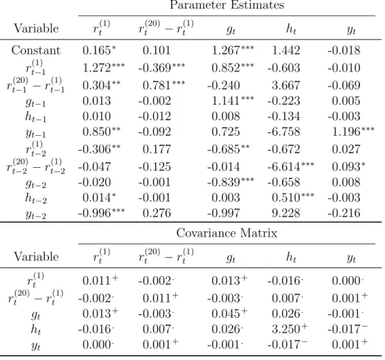
Based on initial values of the five state variables and parameter estimates of the VAR(2) model, we simulate 10,000 paths for each state variable for the sample period 1992-2011. The probability density functions (PDFs) of these simulated values are compared with the historical values of the state variables in Fig. 2. The PDFs of the simulated state variables
using the VAR(2) model are comparable to their empirical distributions, except for rental yields. The historical distribution of rental yields is bimodal, which arises because rental yields in Sydney moved to a lower level after 2001, and the VAR model captures the most recent level in the simulations. However, house price values are found not to be influenced significantly by rental yields in the VAR model3 and rental yields are not used in the later
analysis. We have also performed tests on the residuals of the VAR(2) model. The tests show that the residuals do not have significant auto- or cross-correlations and confirm the fit of the VAR(2) model.
0 1 2 3 0 0.5 1 1.5 (%) rt(1) Historical Simulated −0.5 0 0.5 1 0 0.5 1 1.5 2 (%) r(20)t −r(1)t 0 1 2 3 0 0.2 0.4 0.6 0.8 (%) gt −10 −5 0 5 10 0 5·10−2 0.1 0.15 0.2 (%) ht 0 1 2 0 0.5 1 1.5 2 (%) yt
Fig. 2. PDFs of historical and simulated state variables.
3.3.2 Stochastic discount factors
Following Alai et al. (2014), stochastic discount factors that reflect the key risks in reverse
mortgage cash flows are used to value reverse mortgage loans. The discount factor is modelled
3We have performed a robustness test by estimating a VAR(2) model that excludes rental yields from
the state variables. We find that house price values are not influenced significantly by the inclusion of rental yields in the model.
as: mt+1 = exp −r (1) t −λ 0 tλt−λ0tZt+1 , (14)
where λt is the time-varying market price of risk, which is assumed to be an affine function
of the state variables Yt in the VAR (2) model (Ang and Piazzesi, 2003):
λt =λ0 +λ1Yt. (15)
To derive stochastic discount factors based on the VAR model, zero-coupon bond prices are assumed to be exponential linear functions of contemporaneous and one-quarter lagged state variables (Shao et al., 2012):
pnt = exp(An+B0nYt+Cn0Yt−1), (16)
whereAn,Bnand Cnare parameters that can be solved for using the following simultaneous
difference equations (proof in Shao et al., 2012):
An+1 =An+Bn0(κ−Σ 1/2 λ0) + 1 2B 0 nΣBn, Bn+1 = (Φ1−Σ1/2λ1)0Bn+Cn−e1, Cn+1 = Φ02Bn. (17)
The initial values of the three parameters in Equations (17) are A1 = 0, B1 = −e1, and C1 = 0, wheree1 denotes a vector with the first component of one and other components of zeros. The estimated quarterly yield rate with n quarters to maturity at time t is expressed as ˆrt(n) =−(An+B
0
nYt+C
0
nYt−1)/n. The market price of risk is obtained by minimising the sum of squared deviations of the estimated yield rates from the observed rates:
min λ ( X n ˆ r(tn)−rt(n) 2) . (18)
Table 3. Correlation coefficients between stochastic discount factors and state variables. Variable mt r (1) t r (20) t −r (1) t gt ht yt mt 1.000 r(1) -0.940∗∗∗ 1.000 rt(20)−rt(1) 0.235∗∗ -0.261∗∗ 1.000 gt -0.296∗∗ 0.396∗∗∗ -0.362∗∗∗ 1.000 ht 0.108 -0.298∗∗∗ 0.346∗∗∗ -0.155 1.000 yt -0.315∗∗∗ 0.262∗∗ 0.602∗∗∗ -0.299∗∗∗ 0.202∗ 1.000 ∗ p <0.10; ∗∗ p < 0.05; ∗∗∗ p < 0.01.
Equations (14) and (15) link the stochastic discount factors to the state variables in the VAR model. Table 3 reports the correlations between the estimated stochastic discount factors and the state variables. All correlations, except those with the growth rates of the aggregate house price index, are economically and statistically significant. The estimated stochastic discount factors reflect the risks in the state variables.
3.3.3 Disaggregated house price index projection
Disaggregated house price indices for properties with specific characteristics are then linked to the average house price index using a VAR with exogenous variables (VARX(˜p,q)) model,˜ where the average house price index is the exogenous variable. The model is given by:
hdt = ˜κ+ ˜ p X i=1 ˜ Φi hdt−i+ ˜ q X j=0 ˜ Ωj ht−j + ˜Σ1/2Z˜t, (19) wherehd
t is a vector of growth rates of the disaggregated house price indices, htis the growth
rate of the aggregate house price index, ˜Zt is a vector of independent standard normal
random variables, ˜p is the lag length for the state variables, and ˜q is the lag length for the exogenous variable. The optimal lag lengths for the VARX model are selected based on the three information criteria reported in Table 4. All three criteria suggest that a VARX(1,0) is the optimal specification.
Table 4. Information criteria for VARX models with different lag lengths (˜p,q).˜ Criteria (1,0) (1,1) (1,2) (2,0) (2,1) (2,2) AICc 9.927 10.231 10.533 11.643 12.131 12.366 AIC 9.317 9.504 9.650 9.327 9.428 9.552 BIC 13.025 13.521 14.009 15.977 16.489 16.725
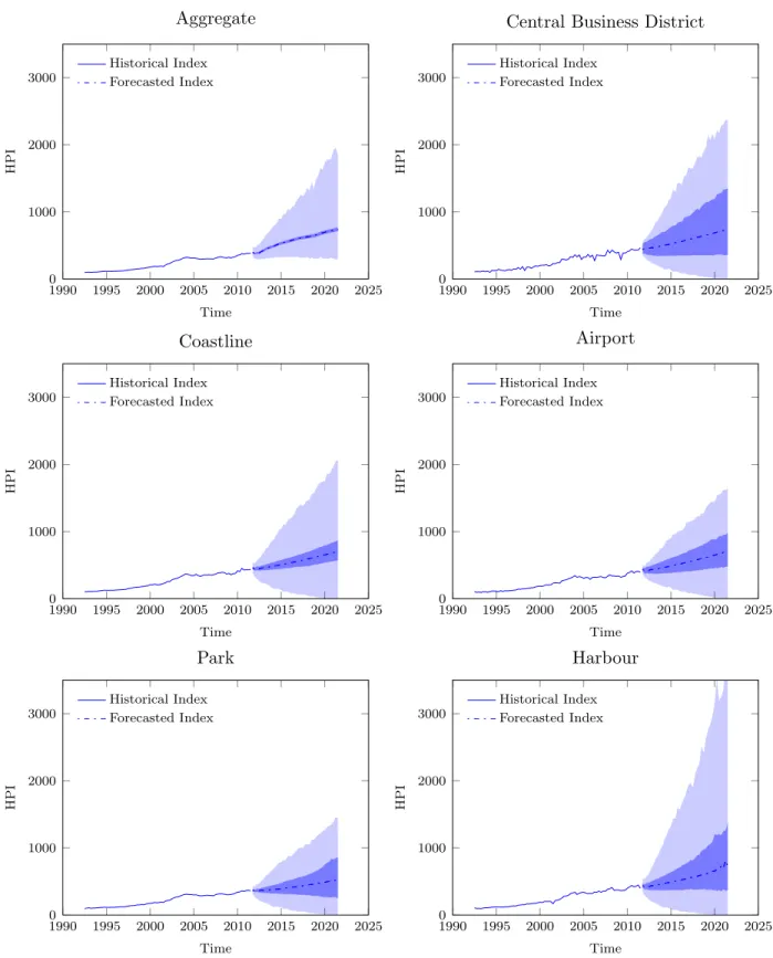
Using the estimates of the VARX(1,0) model, price indices for houses with specific char-acteristics are simulated. The simulation accounts for parameter uncertainty in the VARX model. Parameters in the VARX(1,0) model are assumed to be normally distributed. It is also assumed that parameters in ˜Φi are independent of parameters in ˜Ωj. Fig. 3 shows the
projected aggregate price index for Sydney and the indices for houses located in different regions of Sydney, including the central business district, the coastline, the Sydney harbour, the airport vicinity, and suburbs that have a park. The regional classification is based on the postcode area in Hanewald et al. (2013). The price of houses in these different regions
shows more volatility than the aggregate house price in Sydney.
3.4 Termination of reverse mortgages
Termination triggers of reverse mortgages include mortality, move-out due to health-related issues, voluntary prepayment and refinancing (Ji et al., 2012). To model the different
ter-mination triggers we use a variant of the multi-state Markov model developed by Ji et al.
(2012). Similar models have been used by Alaiet al.(2014) and Choet al.(2013). We extend
this line of research by allowing mortality rates to be random variables. In the following, this section first describes the calibration of the Wills-Sherris stochastic mortality model and the projection of future mortality rates. The modelling of the termination triggers then follows.
1990 1995 2000 2005 2010 2015 2020 2025 0 1000 2000 3000 Time HPI Aggregate Historical Index Forecasted Index 19900 1995 2000 2005 2010 2015 2020 2025 1000 2000 3000 Time HPI
Central Business District
Historical Index Forecasted Index 1990 1995 2000 2005 2010 2015 2020 2025 0 1000 2000 3000 Time HPI Coastline Historical Index Forecasted Index 19900 1995 2000 2005 2010 2015 2020 2025 1000 2000 3000 Time HPI Airport Historical Index Forecasted Index 1990 1995 2000 2005 2010 2015 2020 2025 0 1000 2000 3000 Time HPI Park Historical Index Forecasted Index 19900 1995 2000 2005 2010 2015 2020 2025 1000 2000 3000 Time HPI Harbour Historical Index Forecasted Index
Fig. 3. Projection of price indices for houses in different regions of Sydney. Dark-shaded ar-eas represent 95%-confidence intervals without incorporating parameter uncertainty. Light-shaded areas are 95%-confidence intervals that take into account parameter uncertainty.
3.4.1 Stochastic mortality
Wills and Sherris (2008) develop a multi-variate stochastic mortality model to describe the volatile improvement of mortality rates over time. The model describes changes in age-specific mortality rates along the cohort direction as a function of age, time effects and multiple stochastic risk factors. Observed correlations between the year-to-year changes in mortality rates of different age groups are incorporated in the multivariate distribution of the stochastic risk factors. The Wills-Sherris model allows for a more flexible and realistic age dependence structure than, for example, the one-factor model by Lee and Carter (1992) and the two-factor model by Cairns et al. (2006). An explicit expression for the age dependence
structure can be derived in the Wills-Sherris model. The Wills-Sherris model has been applied in several studies analysing the pricing and risk-management of financial products exposed to longevity risk (see, e.g. Hanewaldet al., 2013; Ngai and Sherris, 2011; Wills and
Sherris, 2010).
The model formulates the changes in log mortality rates along the cohort direction: ∆clnµ(x, t) =
lnµ(x, t)−lnµ(x−1, t−1), where µ(x, t) is the force of mortality for a person aged x at
time t with x=x1, x2,· · ·, xN and t=t1, t2,· · · , tT. These cohort changes in log mortality
rates are assumed as follows:
∆clnµ(x, t) =ax+b+σε(x, t), (20)
wherea,bandσare parameters to be estimated, andε(x, t) follows a standard normal distri-bution that drives the fluctuation of mortality improvements. To account for age dependence, ε(x, t) is expressed as a linear combination of independent standard normal random vari-ables, i.e. εt= [ε(x1, t), ε(x2, t),· · · , ε(xN, t)]0 = Ω
1
2Wt, where Ω is a covariance matrix that
captures the age dependence structure and Wt is a vector of independent standard normal
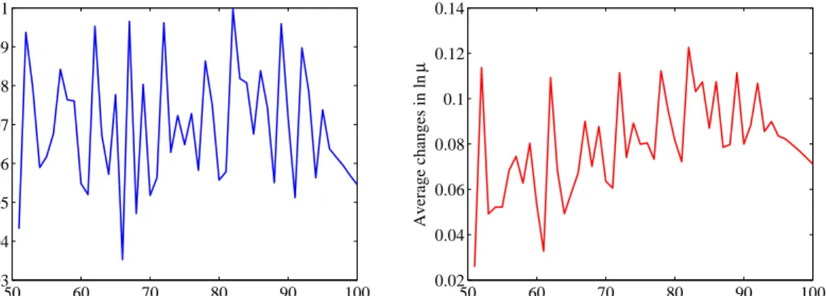
50 60 70 80 90 100 0.03 0.04 0.05 0.06 0.07 0.08 0.09 0.1 Age Average changes in ln µ 50 60 70 80 90 100 0.02 0.04 0.06 0.08 0.1 0.12 0.14 Age Average changes in ln µ
Fig. 4. Average changes in log mortality rates along the cohort direction for different ages for Australian males (left) and females (right), 1970-2009.
In the Wills-Sherris model, the log changes in mortality rates along the cohort direction result from mixed effects that can be decomposed into age and period effects. Fig. 4 shows the average values (averaged over time) of the log changes in mortality rates along the cohort direction for different ages. There is a linear trend in these log changes, providing justification for the specification of the Wills-Sherris model. Similar to the Lee-Carter model and the two-factor CBD model, mortality changes can be decomposed into age and time effects. The decomposition of the mixed effects in the Wills-Sherris model is shown in the following equation:
∆clnµ(x, t) = [ax+b−g(x)] + [g(x) +σε(x, t)], (21)
where g(x) is an implicit function of age that captures the trend of the stochastic improve-ments in mortality rates over time. For example, if g(x) is lower for smaller x, it suggests that mortality improvements are more pronounced for younger ages. In Equation (21), [ax+b−g(x)] is the age effect and [g(x) +σε(x, t)] is the period effect. For mortality pro-jections, we are not interested in the value ofg(x) since the effect of g(x) is cancelled out in the cohort direction.
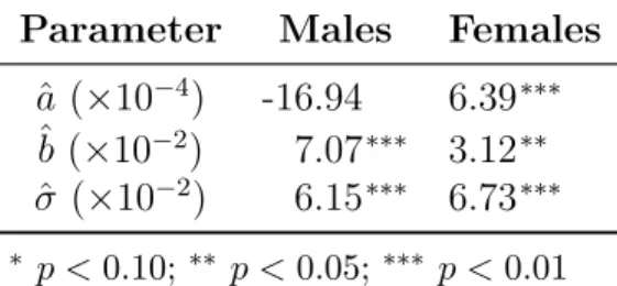
The Wills-Sherris model is estimated for male and female mortality rates for ages 50-100 and years 1970-2009 using a linear regression of Equation (20). The estimated parameters ˆa, ˆb
Table 5. Parameter estimates for the Wills-Sherris model based on data for Australia, 1970-2009.
Parameter Males Females
ˆ a (×10−4) -16.94 6.39∗∗∗ ˆ b (×10−2) 7.07∗∗∗ 3.12∗∗ ˆ σ (×10−2) 6.15∗∗∗ 6.73∗∗∗ ∗ p <0.10; ∗∗ p <0.05; ∗∗∗ p <0.01
Table 6. Covariance matrix of estimated parameters in the Wills-Sherris model.
Parameter Males Females
ˆ a ˆb ˆa ˆb ˆ a 2.36×10⁻⁸ – 3.53×10⁻⁸ – ˆ b -1.78×10⁻⁶ 1.39×10⁻⁴ -2.66×10⁻⁶ 2.08×10⁻⁴
and ˆσ are given in Table 5, and the covariance matrix of the parameters is shown in Table 6. The estimate for a is negative for males but positive for females. This is consistent with Fig. 4, where the log changes in mortality rates show a slightly downward sloping trend for males and an positive trend for females. This pattern implies that over the sample period the changes in log mortality rates along the cohort direction have been larger for males at younger ages and for females at older ages.
The estimated residuals from the Wills-Sherris model based on Australian mortality data for males and females respectively are plotted in Fig. 5. The residuals do not show distinct patterns and are consistent with the assumption of a multi-variate normal distribution. The age dependence structure is estimated as the covariance matrix of the calculated residuals.
To simulate future mortality rates, the Cholesky decomposition of the covariance matrix Σ is required. However, due to the fact that the number of years in the data is smaller than the number of ages, the Cholesky decomposition cannot be directly calculated. Instead, Wills and Sherris (2008) suggest using the eigenvalues and eigenvectors of the covariance matrix.
1975 1980 1985 1990 1995 2000 2005 55 60 65 70 75 80 85 90 95 100 Time Age 1975 1980 1985 1990 1995 2000 2005 55 60 65 70 75 80 85 90 95 100 Time Age
Fig. 5. Binary black-white residuals from the Wills-Sherris model for males (left) and females (right). The horizontal and vertical axes are respectively the age and the time. Black cells indicate negative residuals; white cells indicate non-negative residuals.
Ω has orthogonal eigenvectors, that is:
V V0 =I, (22)
where V is the eigenvector matrix of Ω and I is the identity matrix. According to the property of eigenvectors, the following equation holds:
Ω =VΛV−1 =VΛV0 = (VΛ12)(VΛ 1
2)0, (23)
where Λ is a diagonal matrix of Ω’s eigenvalues.
Equation (23) implies that Ω can be expressed as the product of a matrix and its transpose, which is a generalised Cholesky decomposition. VΛ12 can be used to simulate multi-variate
normal random variables ε(x, t) based on the following equation:
εt = (VΛ
1
2)Wt. (24)
depen-dence structure for these ages is the same as that for age 100. This assumption is justified by the fact that the generalised Cholesky decomposition of the age dependence matrix, VΛ12, is
very stable for ages above 100. Values ofVΛ12 for selected ages are shown in Fig. 6. The top
two panels show the values of VΛ12 respectively for males and females aged 60, 80, 90 and
100, suggesting that the values for these different cohorts are very different. The bottom two panels show the values of VΛ12 for ages 96 to 100. The values for the oldest old are almost
the same and the lines overlap.
50 60 70 80 90 100 0 0.5 1 Age 60 80 90 100 50 60 70 80 90 100 −1 −0.5 0 0.5 1 Age 60 80 90 100 50 60 70 80 90 100 0 0.5 1 Age 96 97 98 99 100 50 60 70 80 90 100 0 0.5 1 Age 96 97 98 99 100
Fig. 6. The generalised Cholesky decomposition of the age dependence matrix for selected ages, males (left) and females (right).
Based on the estimates of parameters in the Wills-Sherris model and the simulated multi-variate random variables, future mortality rates are projected. Male and female cohort
70 80 90 100 110 0 0.2 0.4 0.6 0.8 1 Age Surviv al probabilit y Mean 90% confidence interval 70 80 90 100 110 0 0.2 0.4 0.6 0.8 1 Age Surviv al probabilit y Mean 90% confidence interval
Fig. 7. Simulated survival probabilities of males (left) and females (right) initially aged 65.
survival probabilities derived from the projected mortality rates are shown in Fig. 7.
3.4.2 In-force probabilities
Following Ji et al. (2012) and Cho et al. (2013), we model the different triggers for reverse
mortgage termination but allow mortality rates to be random variables. The mortality rate of borrowers is assumed to be lower than that of the population of the same age, in order to reflect the better health of retirees that still live at home compared to those that have moved to aged care facilities. At-home mortality rates are derived by applying age-specific scaling factors to the population mortality rates (Cho et al., 2013; Jiet al., 2012). The probability
of moving out due to health-related reasons, mainly because of entry into a long-term care (LTC) facility, is assumed to be a proportion of the mortality rate. Furthermore, voluntary prepayment and refinancing are specified as functions of the contract duration in years. These two termination triggers are assumed to be competing risk factors with mortality and LTC incidence.
Table 7. Assumptions on termination triggers adopted from Ji et al. (2012) and Cho et al.
(2013).
Age At-home mortality LTC incidence Prepayment Refinancing scaling factor factor Duration Probability Duration Probability
65-70 0.950 0.100 1-2 0.00% 1-2 1.00% 75 0.925 0.150 3 0.15% 3 2.00% 80 0.900 0.200 4-5 0.30% 4-5 2.50% 85 0.875 0.265 6+ 0.75% 6-8 2.00% 90 0.850 0.330 9-10 1.00% 95 0.825 0.395 11-20 0.50% 100+ 0.800 0.460 21+ 0.25%
of the mortality rate and of other termination factors:
tpcx = exp − Z t 0 (θx+s+ρx+s)ˆµx+sds t Y i=1 h (1−qprei )(1−qiref) i1/4 , (25)
where θx+s is the scaling factor for at-home mortality rates at age x+s, ρx+s is the
age-specific factor that captures LTC incidence, ˆµx+s is the projected quarterly force of mortality
derived from the Wills-Sherris model, qipre is the annual duration-dependent probability of prepayment, and qiref is the annual duration-dependent probability of refinancing. Due to lack of public access to detailed data on these rates or probabilities, assumptions based on the UK experience given in Equity Release Working Party (2005), Hosty et al. (2008), Ji et al.
(2012) and Choet al. (2013) have been employed in this paper. The parameter assumptions
are summarised in Table 7. Furthermore, Equation (25) implies an assumption that the force of termination is constant within one year. Mortality rates are projected on an annual basis in Section 3.4.1. Quarterly mortality rates are obtained by assuming a constant force of mortality between integer ages.
4
Results
We present results calculated based on the projected house price indices and mortality rates to show the impact of idiosyncratic house price risk and of longevity risk on the pricing of reverse mortgages. Robustness tests are performed to test the sensitivity of the results to different mortality models and to the assumptions about non-mortality termination rates.
4.1 Base case results
We model reverse mortgage loans issued to a single 65-year-old female borrower with a property valued at $800,000 at the issuance of the loan. $800,000 is about the 2010 median house price value in the data set we analyse. We assume that the mortgage rate has a quarterly lending margin of 0.4% (Chen et al., 2010): κ = 0.4% in Equation (1). The
transaction cost of selling the property is assumed to be 6 % of the house price, i.e. c= 6%.
In the base case, future mortality rates are projected based on the Wills-Sherris model. Different house price indices for properties with specific characteristics are compared to assess the impact of idiosyncratic house price risk. Panel A of Table 8 reports the results for the case where the house value is modelled using the aggregate house price index for Sydney. Panels B to G report the results for reverse mortgages on houses in the different regions of Sydney as described in Section 3.3.3. Panels H and I illustrate the impact of the property’s number of bathrooms or bedrooms. These house characteristics are identified as important determinants of differences in house price dynamics in Shao et al. (2013). We also compare
three different initial loan-to-value (LTV) ratios (0.2, 0.4 and 0.6) in each panel.
Table 8 reports the annualised value for the mortgage insurance premium rateπ, the value of the NNEG together with the corresponding standard error, and the 95% Tail Value-at-Risk (TVaR) of the provider’s shortfall. The mortgage insurance premium rate π charged for the no-negative equity guarantee is calculated by equating the values for NNEG and MIP. Based
on the value for π, the provider’s actual shortfall SF is calculated allowing for uncertainty in the survival probability as described in Section 3.1. The TVaR of the provider’s shortfall is calculated to show the impact of stochastic mortality rates.
Mortgage insurance premium rates and NNEG values vary substantially across Panels A to I, which shows that location and house characteristics are important factors in impacting the risk of reverse mortgages. Using market-average house price dynamics substantially underestimates the risks for reverse mortgages with LTV ratios of 0.2 and 0.4 written on properties in specific regions of Sydney or with specific characteristics. For these LTV ratios, the mortgage insurance premium, the NNEG value and the TVaR are all higher in Panels B to I than the corresponding values in Panel A.
The comparison gives different results for an LTV ratio of 0.6: in this case, the NNEG value in Panel A, where the Sydney index is assumed, is higher than the NNEG in most other Panels. This can be explained as follows. At a LTV ratio of 0.6, the loan balance is very likely to exceed the house price at termination. The expected loss for the provider in that case is larger when the aggregate index is used because the aggregate index has a lower growth rate and a lower volatility than most of the disaggregated indices (see Fig. 3).
These comparisons show that reverse mortgage providers should model the house price risk in reverse mortgages using house price models that are disaggregated according to the prop-erty’s location and characteristics. The following example illustrates this point. Suppose a reverse mortgage provider issues contracts to several 65-year-old female borrowers with dif-ferent houses represented in Panels B to G of Table 8. We assume the number of properties is the same in each category. Each loan should be charged the corresponding mortgage in-surance premium given in Table 8. The average annual mortgage inin-surance premium for this portfolio is 0.41%. This value (and each individual premium rate) is higher than the annual mortgage insurance premium rate of 0.19% calculated based on the Sydney aggregate index. In this example, pricing based on the Sydney aggregate index substantially undervalues the
no-negative equity guarantee.
4.2 Sensitivity analysis: deterministic mortality
To assess the impact of longevity risk on reverse mortgage pricing, the results obtained using alternative assumptions on the development of future mortality rates are compared. We first consider a simple deterministic mortality model in which future mortality rates are assumed to decrease at age-specific constant rates. The model is given by:
∆ lnµ(x, t) = ∆ lnµx, (26)
where ∆ lnµ(x, t) = lnµ(x, t) −lnµ(x, t − 1) denote the year-to-year change in the log mortality rate at age x and ∆ lnµx is the sample mean of the historical changes in the log
mortality rates. We estimate this model using mortality data for ages 50-100. Data on mortality rates for the oldest old are scanty and the changes in mortality rates are very volatile. We assume that mortality rates for individuals aged 101 - 110 remain constant at the rates in 2009. The assumed age-specific annual decreases in log mortality rates are shown in the left panel of Fig. 8. The implied survival curve derived from the deterministic model is compared with that derived from the Wills-Sherris model in the right panel of Fig. 8. The deterministic model does not account for uncertainty in survival trends and substantially underestimates future mortality improvements compared to the average projection of the Wills-Sherris model.
The first three columns of Table 8 give the mortgage insurance premium rate, NNEG and TVaR values when the deterministic mortality model is adopted. The values for LTV ratios of 0.2 and 0.4 are mostly smaller than those based on the Wills-Sherris model, suggesting that the risk is underestimated when the provider fails to employ an appropriate mortality model to quantify and forecast mortality improvements.
50 60 70 80 90 100 110 −3 −2 −1 0 ·10 −2 Age ∆ ln µx 70 80 90 100 110 0 0.2 0.4 0.6 0.8 1 Age Surviv al probabilit y Deterministic Stochastic mean 90% CI
Fig. 8. Average changes in log mortality rates over time and a comparison of the survival probabilities for a 65-year-old female in the deterministic mortality model and in the Wills-Sherris model.
The main impact of longevity risk on the pricing of reverse mortgages results from the as-sumed trend in mortality improvements rather than from the uncertainty around the trend. This can be seen by comparing the TVaR0.95 values of the lender’s shortfall under the de-terministic mortality model and the Wills-Sherris model. The TVaR0.95 values are small compared to the NNEG and relatively similar under both models. In addition, the impact of longevity risk is smaller than the effect of including idiosyncratic house price risk. A possible explanation is the assumption that longevity risk is not priced in the market and not included in the stochastic discount factors derived from the VAR model.
4.3 Sensitivity analysis: the two-factor Cairns-Blake-Dowd (CBD) model
To further test the results’ sensitivity to the mortality assumptions, the popular two-factor stochastic mortality model developed by Cairns et al. (2006) is also considered. The model
is given by:
logit q(t, x) = κ(1)t +κ(2)t (x−x),¯ (27) where q(t, x) is the death probability of a person aged x at time t, ¯x is the average age in the population, and κ(1)t and κ(2)t capture the period effect.
The residuals from the CBD model estimated for Australian males and females (ages 50-100) are plotted in Fig. 9. The figure shows pronounced clustering of residuals from the CBD model. A possible reason can be the fact that the actual age effect shows more curvature than the logit-linear specification in the two-factor CBD model.
1970 1980 1990 2000 50 60 70 80 90 100 Time Age (a) Male 1970 1980 1990 2000 50 60 70 80 90 100 Time Age (b) Female
Fig. 9. Binary black-white residuals from the CBD model. The horizontal and vertical axes are respectively the age and the time. Black cells indicate negative residuals; white cells indicate non-negative residuals.
The residuals from the Wills-Sherris model and from the two-factor CBD model are com-pared. We average the age-specific residuals over time and calculate their standard devia-tions. The resulting values are shown in Fig. 10. The residuals from the two-factor CBD model are generally smaller and much less volatile than the residuals from the Wills-Sherris model but show patterns in Fig. 9. This reflects the different model assumptions for cohort, period and age trends as well as the different number of factors for volatility and assumptions for dependence between cohorts.
We also compare the projected survival curve for a 65-year-old female based on the CBD model with that based on the Wills-Sherris model. The survival curves are shown in Fig. 11. The survival probabilities projected using the CBD model are much lower than those esti-mated from the Wills-Sherris model and very similar to those calculated from the determin-istic mortality model. For example, the survival probability of a 65-year-old female surviving
50 60 70 80 90 100 −1 0 1 2 Mean, WS Std, WS Mean, CBD Std, CBD 50 60 70 80 90 100 −1 0 1 2 Mean, WS Std, WS Mean, CBD Std, CBD
Fig. 10. Comparison of residuals from the Wills-Sherris model and the two-factor CBD model, males (left) and females (right).
to age 100 is expected to be 0.08 in the deterministic model, 0.10 in the CBD model, and 0.28 in the Wills-Sherris model. The uncertainty around the average survival curves is very comparable in the two stochastic mortality models. For example, the width of the 90% con-fidence interval for the survival probability of a 65-year-old female surviving to age 100 is 0.2 and 0.3 under the CBD model and the Wills-Sherris model, respectively. The corresponding remaining life expectancy of a 65-year-old female is 25 years in the deterministic model, ranges from 22 to 27 years with 90% probability in the CBD model, and ranges from 25 to 31 years with 90% probability in the Wills-Sherris model.
The last three columns of Table 8 show the mortgage insurance premium rates, NNEG and TVaR values based on the CBD model. All values are very close to those calculated based on the deterministic model. The values are generally less than those calculated under the Wills-Sherris model for low LTV ratios (0.2 and 0.4) and greater for high LTV ratios (0.6). These differences are explained by the different longevity trends projected in the Wills-Sherris model. In situations where the accumulated loan amount exceeds the house value (more likely for contracts with high LTV ratios), a longer life expectancy increases the chance that the house price catches up. This effect is comparable to the price of an in-the-money put option: the longer the time to maturity, the lower the price of an in-the-money option and the higher the price of an out-of-the-money option.
Table 8. Valuation of the mortgage insurance premium rateπand the NNEG for reverse mortgages with different loan-to-value (LTV) ratios.
Model Deterministic Wills-Sherris Cairns-Blake-Dowd
LTV 0.2 0.4 0.6 0.2 0.4 0.6 0.2 0.4 0.6
A. Overall Sydney house price index
π(p.a.) 0.003% 0.230% 3.246% 0.009% 0.360% 2.583% 0.003% 0.237% 3.126%
NNEG 71 12,794 400,017 279 22,393 335,952 90 13,147 379,366
S.E. 17 498 2,131 36 639 2,038 18 491 2,094
TVaR 0.000 0.000 0.000 0.467 6.048 12.913 0.179 5.278 13.487
B. Price index for houses near the central business district
π(p.a.) 0.218% 0.720% 1.829% 0.239% 0.711% 1.621% 0.218% 0.716% 1.819%
NNEG 6,043 42,421 186,092 7,298 46,370 181,302 6,036 42,138 184,776
S.E. 470 1,673 4,092 494 1,680 3,876 463 1,651 4,048
TVaR 0.000 0.000 0.000 6.654 17.148 29.594 6.424 17.779 31.168
C. Price index for houses near to coastlines
π(p.a.) 0.076% 0.255% 1.184% 0.088% 0.302% 1.183% 0.076% 0.257% 1.173%
NNEG 2,062 14,238 110,932 2,624 18,645 124,031 2,070 14,284 109,598
S.E. 289 879 2,399 308 939 2,402 286 866 2,359
TVaR 0.000 0.000 0.000 4.387 11.923 21.331 3.893 11.512 22.120
D. Price index for houses near to an airport
π(p.a.) 0.243% 0.492% 0.967% 0.247% 0.484% 0.901% 0.242% 0.491% 0.966%
NNEG 6,748 28,189 88,181 7,570 30,584 90,594 6,735 28,142 87,983
S.E. 565 1,552 3,146 572 1,554 3,087 558 1,538 3,123
TVaR 0.000 0.000 0.000 8.041 19.035 31.435 8.063 19.653 32.754
E. Price index for houses near to a park
π(p.a.) 0.111% 0.494% 2.720% 0.134% 0.596% 2.267% 0.112% 0.495% 2.662%
NNEG 3,049 28,339 311,635 4,051 38,270 280,287 3,076 28,376 302,862
S.E. 350 1,129 3,250 374 1,205 3,059 345 1,110 3,181
TVaR 0.000 0.000 0.000 5.391 13.544 21.830 4.951 13.445 22.989
F. Price index for houses near to harbour
π(p.a.) 0.146% 0.506% 1.754% 0.173% 0.579% 1.652% 0.146% 0.506% 1.729%
NNEG 4,007 29,090 176,722 5,228 37,101 185,682 4,024 29,034 173,539
S.E. 394 1,218 3,075 414 1,285 3,013 386 1,195 3,014
TVaR 0.000 0.000 0.000 6.119 14.260 23.117 5.858 14.269 24.042
G. Price index for all houses excluding B - F
π(p.a.) 0.040% 0.377% 3.392% 0.058% 0.519% 2.649% 0.041% 0.381% 3.291%
NNEG 1,079 21,307 426,785 1,721 32,963 348,165 1,116 21,539 408,843
S.E. 190 801 2,762 211 913 2,574 188 787 2,697
TVaR 0.000 0.000 0.000 2.766 9.418 16.412 2.167 8.928 16.983
H. Price index for houses with less than or equal to two bathrooms
π(p.a.) 0.010% 0.247% 3.078% 0.019% 0.374% 2.485% 0.011% 0.253% 2.968%
NNEG 269 13,752 370,431 561 23,275 318,003 294 14,080 352,317
S.E. 86 566 2,239 99 692 2,148 87 558 2,198
TVaR 0.000 0.000 0.000 1.028 6.913 13.748 0.634 6.170 14.350
I. Price index for houses with more than two bathrooms
π(p.a.) 0.058% 0.418% 2.868% 0.081% 0.540% 2.376% 0.059% 0.420% 2.781%
NNEG 1,577 23,759 335,272 2,412 34,438 298,788 1,612 23,871 321,653
S.E. 209 893 2,871 232 1,005 2,717 205 874 2,807
TVaR 0.000 0.000 0.000 3.391 10.145 17.505 2.914 9.912 18.420
S.E. is the standard error of the NNEG value. TVaR is the Tail Value-at-Risk of the lender’s shortfall at the significance level of 95%. ‘Deterministic’, ‘Wills-Sherris’ and ‘Cairns-Blake-Dowd’ denote different mortality models.
65 70 75 80 85 90 95 100 105 110 0 0.2 0.4 0.6 0.8 1 Age Surviv al probabilit y Deterministic CBD, mean CBD, 90% CI WS, mean WS, 90% CI
Fig. 11. Comparison of survival probabilities of the cohort 65 from the Wills-Sherris model and the two-factor CBD model.
4.4 Sensitivity analysis: LTC incidence, prepayment and refinancing
Other termination triggers such as move-out due to health related reasons, voluntary pre-payment and refinancing are also important risk factors faced by reverse mortgage providers. In the base case analysis we use assumptions on these rates and probabilities shown in Table 7. This section investigates the sensitivity of the base case results by varying the assump-tions on the LTC incidence, prepayment probabilities and refinancing probabilities. Table 9 displays the results.
The numerical results show that the annual mortgage insurance premium rates are stable for different assumptions on these termination rates and probabilities. Even in a joint stress test where the LTC incidence, prepayment probabilities and refinancing probabilities are decreased or increased by 50% at the same time, annual mortgage insurance premium rates show limited variations. The values of the NNEG and the TVaR are also stable in the different scenarios. Based on the results shown in Tables 8 and 9, we conclude that the impact of idiosyncratic house price risk and longevity risk is much larger than that of non-mortality termination triggers like LTC incidence, prepayment and refinancing.
Table 9. Sensitivity analysis: valuation of the mortgage insurance premium π and the NNEG for reverse mortgages for alternative assumptions about LTC incidence, prepay-ment and refinancing probabilities.
Base LTC Incidence Prepayment Refinancing Joint
↓50% ↑50% ↓ 50% ↑50% ↓ 50% ↑50% ↓ 50% ↑50%
A. Overall Sydney house price index
π(p.a.) 0.360% 0.377% 0.337% 0.388% 0.335% 0.384% 0.338% 0.430% 0.293%
NNEG 22,393 24,232 20,315 25,189 19,945 25,974 19,310 31,566 15,665
S.E. 639 657 611 698 585 727 561 814 492
TVaR 6.048 6.067 5.945 6.485 5.642 6.811 5.366 7.290 4.914
B. Houses near the central business district
π(p.a.) 0.711% 0.690% 0.719% 0.719% 0.701% 0.728% 0.692% 0.710% 0.688%
NNEG 46,370 46,433 45,593 48,933 43,952 51,721 41,545 54,367 38,674
S.E. 1,680 1,666 1,673 1,753 1,611 1,855 1,521 1,914 1,453
TVaR 17.148 16.877 17.253 17.625 16.703 18.694 15.732 18.835 15.398
C. Houses near to coastlines
π(p.a.) 0.302% 0.304% 0.296% 0.314% 0.291% 0.315% 0.290% 0.327% 0.272%
NNEG 18,645 19,363 17,727 20,175 17,245 21,076 16,485 23,638 14,517
S.E. 939 946 922 994 888 1,046 842 1,115 784
TVaR 11.923 11.901 11.818 12.540 11.340 13.236 10.733 13.882 10.119
D. Houses near to an airport
π(p.a.) 0.484% 0.471% 0.490% 0.485% 0.482% 0.490% 0.477% 0.475% 0.480%
NNEG 30,584 30,682 30,144 31,914 29,323 33,612 27,821 35,087 26,291
S.E. 1,554 1,542 1,550 1,607 1,504 1,697 1,423 1,740 1,376
TVaR 19.035 18.779 19.133 19.476 18.627 20.627 17.573 20.746 17.282
E. Houses near to a park
π(p.a.) 0.596% 0.596% 0.583% 0.625% 0.568% 0.627% 0.565% 0.652% 0.526%
NNEG 38,270 39,580 36,289 41,942 34,964 43,894 33,365 49,497 28,943
S.E. 1,205 1,208 1,187 1,280 1,137 1,349 1,076 1,433 1,001
TVaR 13.544 13.419 13.530 14.132 12.991 14.979 12.241 15.458 11.720
F. Houses near to harbour
π(p.a.) 0.579% 0.578% 0.569% 0.603% 0.556% 0.606% 0.553% 0.625% 0.519%
NNEG 37,101 38,295 35,347 40,351 34,141 42,258 32,559 47,240 28,569
S.E. 1,285 1,288 1,265 1,365 1,210 1,440 1,146 1,530 1,063
TVaR 14.260 14.099 14.248 14.926 13.622 15.821 12.844 16.306 12.247
G. All houses excluding B - F
π(p.a.) 0.519% 0.530% 0.496% 0.554% 0.486% 0.552% 0.487% 0.597% 0.435%
NNEG 32,963 34,840 30,535 36,809 29,573 38,235 28,428 44,928 23,692
S.E. 913 924 890 983 850 1,032 808 1,120 734
TVaR 9.418 9.390 9.335 9.957 8.906 10.514 8.429 11.047 7.892
H. Houses with less than or equal to two bathrooms
π(p.a.) 0.374% 0.389% 0.352% 0.401% 0.348% 0.398% 0.351% 0.441% 0.307%
NNEG 23,275 25,048 21,234 26,087 20,804 26,946 20,107 32,439 16,458
S.E. 692 709 666 751 639 785 610 870 543
TVaR 6.913 6.945 6.797 7.373 6.482 7.758 6.156 8.274 5.670
I. Houses with more than two bathrooms
π(p.a.) 0.540% 0.549% 0.521% 0.574% 0.509% 0.573% 0.509% 0.612% 0.461%
NNEG 34,438 36,185 32,138 38,214 31,075 39,776 29,816 46,166 25,157
S.E. 1,005 1,015 981 1,083 934 1,137 888 1,232 805
TVaR 10.145 10.073 10.106 10.723 9.606 11.337 9.075 11.846 8.544
S.E. is the standard error of the NNEG value. TVaR is the Tail Value-at-Risk of the lender’s shortfall at the significance level of 95%. The LTV ratio is 0.4 and mortality is forecasted based on the Wills-Sherris
5
Conclusions
This paper investigates the pricing and risk analysis of reverse mortgages allowing for id-iosyncratic house price risk and longevity risk. The impact of idid-iosyncratic house price risk and longevity risk are shown to be substantial.
To model idiosyncratic house price risk, disaggregated house price indices are constructed using the hybrid hedonic-repeat-sales house price model developed in Shao et al. (2013). A
VAR(2) model is employed to generate economic scenarios that include projections of a city-level house price index. Based on the VAR model stochastic discount factors that reflect the macroeconomic risks impacting reverse mortgage cash flows are calculated. Disaggregated house price indices are projected using a VARX(1,0) model with the aggregate house price index as the exogenous variable. The Wills-Sherris stochastic mortality model is calibrated and employed to forecast future mortality rates. Other termination triggers, including move-out due to health related reasons, voluntary prepayment and refinancing, are linked to the projected stochastic mortality rates.
We find that pricing reverse mortgages based on an average house price index substantially underestimates the risks underwritten by the provider for low loan-to-value ratios of 0.2 and 0.4. Failing to accurately incorporate the cohort trend of improvements in mortality rates also underestimates the risk for low LTV ratios. Opposite effects are found for a high LTV ratio of 0.6. These results agree with the findings of Alai et al.(2014), who find that reverse
mortgages with LTV ratios of over 50% have different risk profiles than contracts with lower loan to value ratios.
Our results are also in line with other studies that focus on analysing the impact of longevity risk on reverse mortgage pricing and risk management. Li et al. (2010) compare NNEG
values using period life tables for 2007 and a cohort life table derived from the Lee-Carter model. They find that NNEG values are typically larger when cohort life tables are used,
but the differences are not statistically significant. Wang et al. (2008) and Yang (2011)
analyse the securitisation of longevity risk in reverse mortgages. Wang et al. (2008) focus
on longevity bonds for reverse mortgages. They test the sensitivity of the present value of the bond values to different mortality assumptions and find that the impact of mortality shocks is very limited. Yang (2011) develops “collateralised reverse mortgage obligations”. She compares the fair spreads for different tranches using the two-factor CBD model, the Lee-Carter model and a static mortality table. She finds that assuming a static mortality table overestimates the fair spread for all tranches, with differences of up to 30% for the senior tranche.
The study provides new and improved insights into the design of reliable and affordable home equity release products. The results suggest that risk factors associated with a property’s characteristics should be used in the pricing and risk analysis of reverse mortgage loans. In particular, the three most important risk factors are the location, the number of bathrooms and the land area. In addition, the results show that a stochastic mortality model based on cohort trends, such as the Wills-Sherris model, should be employed to take into account longevity risk in reverse mortgage loans.
Acknowledgement
The authors acknowledge the financial support of the Australian Research Council Centre of Excellence in Population Ageing Research (project number CE110001029). Shao also acknowledges the financial support from the Australian School of Business and the China Scholarship Council. Opinions and errors are solely those of the authors and not of the institutions providing funding for this study or with which the authors are affiliated.
References
Alai, D., Chen, H., Cho, D., Hanewald, K., and Sherris, M. (2014). Developing equity release markets: Risk analysis for reverse mortgages and home reversions.North American Actuarial Journal,18(1), 217–241.
Andreeva, M. (2012). About mortality data for Australia. Technical report, Human Mortality Database.
Ang, A. and Piazzesi, M. (2003). A no-arbitrage vectorautoregression of term structure dynamics with macroeconomic and latent variables. Journal of Monetary Economics,
50(4), 745–787.
Blackburn, C. and Sherris, M. (2013). Consistent dynamic affine mortality models for longevity risk applications. Insurance: Mathematics and Economics,53(1), 64–73.
Bourassa, S. C., Hamelink, F., Hoesli, M., and MacGregor, B. D. (1999). Defining Housing Submarkets. Journal of Housing Economics,8(2), 160–183.
Bourassa, S. C., Hoesli, M., and Peng, V. S. (2003). Do housing submarkets really matter?
Journal of Housing Economics, 12(1), 12–28.
Bourassa, S. C., Hoesli, M., Scognamiglio, D., and Zhang, S. (2011). Land leverage and house prices. Regional Science and Urban Economics, 41(2), 134–144.
Cairns, A. J., Blake, D., and Dowd, K. (2006). A two-factor model for stochastic mortality with parameter uncertainty: Theory and calibration. Journal of Risk and Insurance,
73(4), 687–718.
Calza, A., Monacelli, T., and Stracca, L. (2013). Housing finance and monetary policy.
Journal of the European Economic Association, 11(s1), 101–122.
Case, B. and Quigley, J. M. (1991). The dynamics of real estate prices. The Review of Economics and Statistics,22(1), 50–58.
Chen, H., Cox, S. H., and Wang, S. S. (2010). Is the home equity conversion mortgage in the United States sustainable? Evidence from pricing mortgage insurance permiums and non-recourse provisions using the conditional Esscher transform. Insurance: Mathematics and Economics, 46(2), 371–384.
Chinloy, P. and Megbolugbe, I. F. (1994). Reverse mortgages: Contracting and crossover risk. Real Estate Economics, 22(2), 367–386.
Cho, D., Sherris, M., and Hanewald, K. (2013). Risk management and payout design of re-verse mortgages. UNSW Australian School of Business Research Paper No. 2013ACTL07. Cocco, J. F. and Gomes, F. J. (2012). Longevity risk, retirement savings, and financial
innovation. Journal of Financial Economics, 103(3), 507–529.
Consumer Financial Protection Bureau (2012). Reverse mortgages: Report to Congress. Available at http://www.consumerfinance.gov/reports/ reverse-mortgages-report/.
Deloitte and SEQUAL (2012). Media Release: Australia’s reverse mortgage market reached $3.3bn at 31 December 2011. Deloitte SEQUAL Research Report.
Englund, P., Quigley, J. M., and Redfearn, C. L. (1998). Improved price indexes for real estate: Measuring the course of Swedish housing prices. Journal of Urban Economics,
44(1), 171–196.
Equity Release Working Party (2005). Equity release report 2005: Technical supplement on pricing considerations. Technical report, Institute and Faculty of Actuaries, U.K. Available at http://www.actuaries.org.uk/research-and-resources/documents/ equity-release-report-2005-volume-2-technical-supplement-pricing-co.
Ferreira, F. and Gyourko, J. (2012). Heterogeneity in neighborhood-level price growth in the United States, 1993-2009. The American Economic Review, 102(3), 134–140.
Goodhart, C. and Hofmann, B. (2008). House prices, money, credit, and the macroeconomy.
Oxford Review of Economic Policy, 24(1), 180–205.
Granados, J. et al. (2008). Macroeconomic fluctuations and mortality in postwar Japan.
Demography, 45(2), 323–343.
Gupta, R., Jurgilas, M., Kabundi, A., and Miller, S. M. (2012). Monetary policy and hous-ing sector dynamics in a large-scale Bayesian vector autoregressive model. International Journal of Strategic Property Management,16(1), 1–20.
Hanewald, K. (2011). Explaining mortality dynamics: The role of macroeconomic fluctua-tions and cause of death trends. North American Actuarial Journal,15(2), 290–314.
Hanewald, K. and Sherris, M. (2013). Postcode-level house price models for banking and insurance applications. Economic Record,89(286), 411–425.
Hanewald, K., Piggott, J., and Sherris, M. (2013). Individual post-retirement longevity risk management under systematic mortality risk. Insurance: Mathematics and Economics,
52(1), 87–97.
Hirata, H., Kose, M. A., Otrok, C., and Terrones, M. E. (2012). Global house price fluctua-tions: Synchronization and determinants. National Bureau of Economic Research Working Paper 18362.
Hosty, G. M., Groves, S. J., Murray, C. A., and Shah, M. (2008). Pricing and risk capital in the equity release market. British Actuarial Journal, 14(1), 41–91.
Iacoviello, M. (2005). House prices, borrowing constraints, and monetary policy in the business cycle. American Economic Review, 95(3), 739–764.
Ji, M., Hardy, M., and Li, J. S.-H. (2012). A semi-Markov multiple state model for reverse mortgage terminations. Annals of Actuarial Science,6(2).
Lee, R. D. and Carter, L. R. (1992). Modeling and forecasting U.S. mortality. Journal of the American Statistical Association, 419(2), 659–671.
Lee, Y.-T., Wang, C.-W., and Huang, H.-C. (2012). On the valuation of reverse mortgages with regular tenure payments. Insurance: Mathematics and Economics, 51(2), 430–441.
Li, J. S.-H., Hardy, M. R., and Tan, K. S. (2010). On pricing and hedging the no-negative-equity guarantee in no-negative-equity release mechanisms. Journal of Risk and Insurance, 77(2), 499–522.
Ngai, A. and Sherris, M. (2011). Longevity risk management for life and variable annu-ities: The effectiveness of static hedging using longevity bonds and derivatives. Insurance: Mathematics and Economics,49(1), 100–114.
Quigley, J. M. (1995). A simple hybrid model for estimating real estate price indexes. Journal of Housing Economics,4(1), 1–12.
Ruhm, C. J. (2007). A healthy economy can break your heart. Demography,44(4), 829–848.
Shao, A. W., Sherris, M., and Hanewald, K. (2012). Equity release products allowing for individual house price risk. In Proceedings of the 11th Emerging Researchers in Ageing Conference, Brisbane, Australia.
Shao, A. W., Sherris, M., and Hanewald, K. (2013). Disaggregated house price indices. UNSW Australian School of Business Research Paper No. 2013ACTL09.
Sherris, M. and Sun, D. (2010). Risk based capital and pricing for reverse mortgages revisited. UNSW Australian School of Business Research Paper No. 2010ACTL04.
Wang, L., Valdez, E. A., and Piggott, J. (2008). Securitization of longevity risk in reverse mortgages. North American Actuarial Journal, 12(4), 345–371.
Wills, S. and Sherris, M. (2008). Integrating financial and demographic longevity risk models: An Australian model for financial applications. UNSW Australian School of Business Research Paper No. 2008ACTL05.
Wills, S. and Sherris, M. (2010). Securitization, structuring and pricing of longevity risk.
Insurance: Mathematics and Economics, 46(1), 173–185.
Yang, S. S. (2011). Securitisation and tranching longevity and house price risk for reverse mortgage products. The Geneva Papers on Risk and Insurance-Issues and Practice,36(4), 648–674.