Disclosure through multiple disclosure channels

(1)

(2)

DISCLOSURE THROUGH MULTIPLE DISCLOSURE CHANNELS

BY

RICHARD M. CROWLEY

DISSERTATION

Submitted in partial fulfillment of the requirements for the degree of Doctor of Philosophy in Accountancy

in the Graduate College of the

University of Illinois at Urbana-Champaign, 2016

Urbana, Illinois

Doctoral Committee:

Professor A. Rashad Abdel-Khalik, Chair Professor Timothy C. Johnson

Professor W. Brooke Elliott Associate Professor Qintao Fan Assistant Professor Wei Zhu

(3)

ABSTRACT

This study examines the impact of managers having a choice of disclosure channels through which they can voluntarily disclose.

This first chapter presents a model in which the manager can choose to disclose different information to two different investor types: informed and uninformed. Firm value is ini-tially established in a competitive equilibrium setting with risk averse investors and noisy information based on the participants’ expectations of firm value given the manager’s dis-closure (or lack thereof). Long-run firm value is established through a rational expectations equilibrium. This paper demonstrates a situation in which the manager will, in equilibrium, disclose more information to informed investors than to uninformed investors some of the time. Furthermore, this paper shows that the manager increases overall disclosure when provided with a second information channel, but decreases disclosure that is quickly parsed by uninformed investors. As the manager’s optimal strategy is identical for maximizing both short and long-run stock price, the manager is able to use multiple disclosure channels to maximize short-run gain without decreasing the long-run stock price.

The second chapter considers the dissemination of information across multiple channels, and the extent to which the use of multiple disclosure channels affects firm stock price. I examine two channels of voluntary disclosures: the voluntary portions of SEC filings and firm websites. Investors appear to react differently to these channels, as SEC filings are likely to be more costly for investors to process (in terms of both acquisition and cognitive costs) when compared to firm websites. These textual voluntary disclosures are examined using a topic modeling methodology to identify two constructs: tone difference, defined as the extent to which firm websites have more positive disclosure and less negative disclosure than SEC filings, and disclosure distance, defined as the extent to which the disclosure topics discussed are similar or different across SEC filings and firm websites. Shifting of information across channels is identified, as some managers appear to voluntarily disclose similar information across these two channels, but with more bad news disclosed through SEC

(4)

filings and more good news disclosed through firm websites. In the short run, asymmetry in processing costs leads to investors impounding the good news in firm websites more quickly than the bad news in the voluntary portion of SEC filings, despite information across channels being released contemporaneously. I find that managers are incentivized to make strategic disclosure channel choices through their stock and option holdings. Furthermore, managers at firms exhibiting strategic disclosure choices sell significantly more stock after the good news is impounded but before the bad news is fully impounded. Further evidence demonstrates that low liquidity helps to facilitate the effects of strategic disclosure channel choices.

(5)

ACKNOWLEDGEMENTS

I would particularly like to thank Professor A. Rashad Abdel-Khalik, who brought me into the program and mentored me from day one. I would also like to thank Professor W. Brooke Elliott, who has advised me and provided much needed research support over the past few years, along with the rest of my dissertation committee who provided me with helpful feedback throughout the process.

I sincerely thank the late Professor Lars Ola Bengtsson. It was his guidance and com-passion that led me into academia, and for that I will be forever grateful.

Lastly, I would like to thank those that have been alongside me during the entire disser-tation process – my loving wife, Yi Liu, along with my wonderful colleagues.

(6)

1 Voluntary Disclosure With

Multiple Channels and Investor

Sophistication

1.1

Introduction

The model detailed in this paper directly addresses a concern of Francis, Nanda & Olsson (2008): determining when managers use different channels of disclosure. By allowing the manager to choose between two channels and not releasing the information at all, the model can build a theory for when a manager will choose one channel over another for a voluntary disclosure.

The model in this paper builds on the basic structure of Dye (1998), a model containing two investor types with one channel of information. This paper provides a useful comparison to see how management may make different decisions when given the opportunity to disclose through multiple channels. Disclosing through multiple channels has become a common oc-currence, with many companies making disclosures through traditional channels such as SEC filings and conference calls, as wells as through newer channels such as websites and social media. As early as 1995, the U.S. Securities and Exchange Commission (SEC) maintained a policy on electronic disclosure (SEC, 1995). In 2000, the use of firm websites for disclosure was specifically discussed (SEC, 2000), and in 2013 the SEC approved of the use of social media networks, such as Twitter and Facebook, as a channel for firm disclosure (SEC, 2013).

(9)

The model takes a basic structure under which the firm is either good or bad, i.e., a market for lemons (Akerlof, 1970). No one in the model knows whether the firm is good or not, but the manager probabilistically receives a signal from the firm that follows the distribution of the firm’s type. This signal could be thought of as a forecast about the potential value of a follow-on project, or another indicator that should be correlated with firm type but not correlated with firm value conditional on knowing the firm type. This signal does not tell the manager the actual value of the firm, but it is useful in determining whether the firm is good or bad. The manager then has the option to disclose or to not disclose the information publicly. If the manager chooses to disclose the information, the manager can then choose to disclose it through an easy-to-process disclosure channel (easy channel) or a hard-to-process disclosure channel (hard channel). In the short run, informed investors see all information that was disclosed, while uninformed investors only see the information that was released via the easy channel. As in Dye (1998), if the manager receives information but chooses not to disclose it through either channel, then the informed investors are aware that the information exists, but they do not know what the information is, whereas the uninformed investors have no information. If the manager receives no information, the informed investors likewise know this, whereas the uninformed investors again have no information. A diagram of the flow of information in this system is presented in Figure 1.1.

Under this framework, the manager does take advantage of this second channel when the manager’s signal is in an intermediate range. Above this range the manager chooses to disclose in the easy channel, and below the intermediate range the manager will choose to withhold information. When the second channel is not present, the manager will withhold information whenever the signal falls below a certain cutoff, which happens to fall in the intermediate range. This result agrees with the primary result of Dye (1998). After de-riving the expected management disclosure pattern, general expressions for the competitive equilibrium price are obtained.

(10)

in-vestors, however, are able to completely discern the informed investors’ information from the initial price, and thus all investors have the same information in the long run. Overall, the long-run results imply that managers can use multiple channels of disclosure to increase firm value in the short run without affecting firm value in the long run.

Through simulation, unconditional expected firm value is examined, as are the dynamics of the equilibrium price and management actions.

Related literature on informed investors in voluntary disclosure is discussed in the next section. In Section 1.3, the general structure of the model is described. Section 1.4 derives the main model and replicates the results of Dye (1998) under the analytical framework described in Section 1.3. Section 1.5 examines implications of the model as well as the dynamics of the equilibrium. Lastly, Section 1.6 concludes. Proofs not included inline are included at the end of the chapter.

1.2

Review of theory

Most of the research on voluntary disclosure focuses on the unraveling result (Grossman & Hart, 1980; Grossman, 1981; Milgrom, 1981; Milgrom & Roberts, 1986), altering one or more of the six conditions for full disclosure. The most pertinent element of the unraveling result to this study is the uniformity of investor response. Suijs (2007) found that violating this condition while holding all others constant is sufficient to induce less than full disclosure. A specific variant of violating uniform investor response that has been considered is varying investor sophistication. Dye (1998) uses rational investors with probabilistic information acquisition, finding that managers disclose more when investors have a higher probability of acquiring information. Fishman & Hagerty (2003) demonstrates a model with two levels of sophistication, where one level is capable of interpreting disclosures and the other only knows the disclosure happened.

The endogenous model in this study builds upon these models by having two separate channels of information: an easy-to-process disclosure channel which can be quickly processed by all investors, and a hard-to-process disclosure channel which can only be quickly processed

(11)

by sophisticated investors. The hard channel can be processed by all investors in the long run, however. Furthermore, the information that can be quickly processed by the unsophisticated investors is not determined probabilistically, but is determined endogenously by the manager. This paper is also related to the stream of literature on limited investor attention. Limited attention has been modeled in the disclosure literature to examine how investors might react to different disclosure formats and rules (Hirshleifer & Teoh, 2003), as well as earnings news (Hirshleifer, Lim & Teoh, 2011). Empirically, some extent of limited investor attention has been documented by Dellavigna & Pollet (2009), showing that stock prices react more slowly to information on Fridays. Likewise, Barber & Odean (2008) empirically demonstrate that investors are more likely to purchase than sell stocks due to attention grabbing news, as investors holding the stock are likely to be paying closer attention to firm news. In this paper, it is assumed that the uninformed investors can only quickly process the easy-to-process disclosure channel, while the informed investors can quickly easy-to-process both channels. While this is a strong use of limited attention, such a strong use is needed to maintain tractability.

1.3

Model structure

The first model takes place in a one period setting in which there are two types of players, a manager and investors, as well as two disclosure channels. The model focuses only on one firm and one manager. The number and types of investors are taken to be exogenous, with 𝑁𝑈 uninformed investors and𝑁𝐼 informed investors,𝑁 investors in total. At the start of the

first period, the firm type is chosen to be either good or bad; the firm is good with probability 𝑝𝐺. If the firm is good (bad), its expected value at time 1 will follow a normal distribution

with mean 𝜇𝐺 (𝜇𝐵) and variance 𝜎𝐻2 (𝜎𝐵2). For simplicity, assume that 𝜎𝐻 = 𝜎𝐵 = 𝜎. A

signal ˜𝑦 exists, such that the signal follows the true distribution of the firm; thus, if the firm is good, ˜𝑦 ∼𝑁(𝜇𝐺, 𝜎2). It is assumed that the manager knows the value of the signal

with some probability, call it ˆ𝑝, as in Dye (1985), Jung & Kwon (1988), and Dye (1998). If the manager knows the value of the signal, then the manager can choose whether or not

(12)

to release the signal. If the manager chooses to release the signal, the manager will then choose which channel to release the signal through. Investors then receive information based on their type and the channel chosen by the manager, determine their desired amount of shares at each possible share price, and trade in order to establish a firm price. Note that this model assumes that the manager does not manipulate the content of any disclosure, as in Dye (1985), Jung & Kwon (1988), and Dye (1998). Consequently, this model assumes that the disclosure content must be the same regardless of the manager’s disclosure channel choice. While this is an idealized case, it is reasonable to assume the same regulations hold across channels. Per SEC Release No. 33-7856 (SEC, 2000), the disclosing party is responsible for the accuracy of the disclosures regardless of the medium through which the statement is made.

1.3.1

Model setup

1.3.1.1 Information

This paper assumes multiple channels of information in the market, as opposed to one channel. By allowing for multiple channels, voluntary disclosures can have different costs of access at the manager’s discretion. The general model in this paper implements this by hav-ing two sets of information, an easy channel and a hard channel. If the two investor groups have a different ability to process these disclosures, then the manager could potentially use this structure for personal gain. Given that firm disclosures naturally vary in readability based on the source, it is quite feasible that disclosure channels will vary in the ease of pro-cessing across investor types. For instance, annual reports tend to have low readability (Li, 2008), whereas disclosures via social media are likely to be more readable. Based on the information that the investors receive, a price per share of the firm, 𝑃0, will be determined.

1.3.1.2 Investors

As with the information, there are two types of investors. The first type of investor (henceforth informed investors) has sufficient processing capability to quickly process all

(13)

information voluntarily released by the manager.1 _{Consequently, this investor sees all}

infor-mation in both channels. Furthermore, this investor type is aware of whether the manager received a signal or not (as in Dye (1998)).2 _{The second type of investor (uninformed}

in-vestors) is able to quickly process only the information disclosed through the easy channel. This investor, however, is not capable of quickly processing the information in the hard channel, i.e., the cost to process the hard channel is too high. All investors’ expected utility is based on their expectation of the underlying value of the firm, the amount of the stock they purchase, and the amount of the risk-free asset that they hold. The risk-free asset is assumed to provide a return plus 1 of 𝑅𝑓 and is perfectly elastic in terms of quantity.

Furthermore, it is assumed that the investors are risk averse, with a utility function follow-ing constant absolute risk aversion (CARA), and in particular the investors have a utility function 𝑈(𝑥) = −𝑒−𝑎𝑥_{, where} _{𝑎 >}_{0 is the coefficient of risk aversion.}3

1.3.1.3 Manager

The model assumes the presence of just one firm with one manager. Inside the firm there is private information in the form of a signal, ˜𝑦, related to the expected value of the firm at time 1. The manager then receives this information with some probability ˆ𝑝 in a noisy manner, receiving the signal ˜𝑦 =𝑦+ ˜𝜖. The signal ˜𝑦 follows the distribution for the actual firm type, which provides information about the firm type in a Bayesian sense. If the firm is good, firm value at time 1 ( ˜𝑃1) and ˜𝑦 will follow𝑁(𝜇𝐺, 𝜎2); if the firm is bad, ˜𝑃1 and ˜𝑦 will

follow 𝑁(𝜇𝐵, 𝜎2). When the manager receives the signal, the manager will decide whether

or not to disclose the information based on the information the manager has, the manager’s utility function, and the expected interpretation and actions by other market participants.

1_{Quickly, in this context, is taken to mean within the time-frame between disclosure and trading.} 2_{This condition is required in order to induce partial disclosure, as otherwise the manager has no incentive} to treat the two types of investors differently, as the investor types would be indistinguishable under a no disclosure case.

3_{This form of utility is used as it allows for tractability when the information processes described in the} next section are normally distributed.

(14)

If the manager chooses to disclose information, the manager must pick between the easy and hard channels to disclose through. While the manager could disclose through both channels simultaneously, doing so is equivalent to disclosing through only the easy channel in this setting, given the investors’ information acquisition processes. The manager’s utility is assumed to be risk neutral and linearly increasing in the initial stock price,𝑃0, of the firm.

1.4

Main model

While deriving the main model, it is helpful to set a baseline by examining a model with one disclosure channel. Such a model is analogous to Dye (1998). However, the model in Dye (1998) is under different assumptions. There are four primary differences between the assumptions detailed in Section 1.3 and the assumptions detailed in the symmetric Bayesian Nash equilibrium of Dye (1998). First, this paper uses a trading model, and consequently includes a risk-free asset along with the risky asset of the firm. Second, the signal in Dye (1998) is the firm value, rather than a random signal from the firm value’s distribution. This difference is needed in order to maintain tractability.4 _{Third, the makeup}

of investors is pre-determined, with 𝑁𝐼 informed investors and 𝑁𝑈 uninformed investors.

Again, this assumption improves tractability.5 _{Lastly, for tractability, firm value follows a}

normal distribution as opposed to a general distribution with a weakly decreasing probability density function (PDF) and investors are risk averse as opposed to risk neutral. These assumptions flow from the standard setup of a competitive equilibrium market pricing model (Grossman, 1976). Given these changes, it is important to verify that the base results of Dye (1998) hold under this new framework, particularly that the manager can have an incentive

4_{Under the Dye (1998) framework, introducing a second disclosure channel leads to an intractable} dis-tribution of bids for uninformed investors. Likewise, under a standard competitive equilibrium in which the signal is the firm value, the expected utility under any withholding case becomes intractable as the distri-bution of expected firm values follow a distridistri-bution akin to a product of a normal PDF and normal CDF weighted to integrate to 1.

5_{In particular, this assumption removes the need to sum across a binomial distribution to get the expected} investor reactions.

(15)

to not fully disclose to all market participants when some participants are informed and some participants are uninformed (this is discussed in Corollary 2.1). Under the framework outlined above, a short run competitive equilibrium can be determined.

Definition 1 (Competitive equilibrium). A competitive equilibrium for the model is the set of manager actions and investor actions covering all possible states of nature, namely whether the manager receives a signal and, if so, the value of the signal. Furthermore, the manager’s actions must lead to the highest price 𝑃0 given the optimal actions of the investors, and the

investors must maximize their expected utility with respect to their own information sets. The uninformed investors’ information set includes whether or not a disclosure was made through the easy channel, and if so, what the signal was. The informed investors’ information set includes whether or not the manager received a signal, whether or not the manager disclosed a signal through either channel, and if so, what the value of the signal was.

This competitive equilibrium can be thought of as follows. Suppose that the manager understands the structure of the market and strategically discloses to maximize the outcome of a one period auction in which all shares must be sold. Then, investors use the information they receive (either the disclosure or the lack thereof), and participate in a silent auction in which the highest price that clears all market shares is chosen. As such, the investors cannot obtain information from the auction itself, as the moment any usable information is generated, i.e., the market clearing price, the auction ends. An extended version of this auction structure is considered in Section 1.4.3.

Initially, there are four states to consider: a signal is obtained by the manager and disclosed to all investors (Full Disclosure, 𝐹 𝐷), a signal is obtained but is disclosed only to informed investors (Partial Disclosure, 𝑃 𝐷), a signal is obtained and is not disclosed (Withholding, 𝑊), and no signal is obtained (No Information, 𝑁 𝐼). As in Dye (1998), the manager may have an incentive not to disclose if the signal ˜𝑦is low enough. This causes the manager’s non-disclosure signal to not be a credible signal of having no information among investors. If the manager could credibly contract to disclose the signal at any value of ˜𝑦,

(16)

non-disclosure could be a credible signal. Without such a contract, there may instead exist a stable point 𝑐𝑊 at which the manager is indifferent between full disclosure and withholding

when ˜𝑦 = 𝑐𝑊. Existence of 𝑐𝑊 is equivalent to the manager having an incentive to not

fully disclose under a one channel model. Furthermore, there may be two additional stable points: one where the manager is indifferent between partial disclosure and full disclosure (when ˜𝑦 = 𝑐𝐹 𝐷) and one where the manager is indifferent between partial disclosure and

withholding (when ˜𝑦 = 𝑐𝑃 𝐷). These two points, 𝑐𝐹 𝐷 and 𝑐𝑃 𝐷, will define the manager’s

incentives under equilibrium. Thus, all four states are possible in this setup: 3 states when the manager receives a signal and one when the manager does not.

Before deriving the equilibrium, an existence condition and uniqueness are discussed.

Theorem 1 (Existence of a non-degenerate solution, competitive equilibrium). A non-degenerate solution for a competitive equilibrium as described in Definition 1 requires a high value of 𝑦˜to be indicative of a good firm and a low value of 𝑦˜ to be indicative of a bad firm. A non-degenerate solution exists whenever the manager’s preferred action for all 𝑦˜ above some point 𝑦¯is to fully disclose. A non-degenerate solution is found whenever the following condition holds: 𝜇𝐺−𝜇𝐵>2𝑎𝑝𝐺 ¯ 𝑥 𝑁𝜎 2_.

Proof. See Section 1.7.1.

This existence criterion is intuitive. While the expected value of ˜𝑃1 is greater under full

disclosure for high values of ˜𝑦, the variance will also be higher. As the investors are risk averse, they do not only care about the difference in the means, but also in the variance of the outcome. The price is penalized by a function that is increasing in the risk aversion of investors and the number of shares available per investor. As risk aversion increases, investors will decrease their willingness to pay for a share of the firm as they will be less willing to take on the risk of the asset. Likewise, as the variances increase, investors will assess a greater

(17)

penalty. As 𝑝𝐺 increases, the difference between the expectation of ˜𝑃1 conditional on ˜𝑦 and

the unconditional expectation of ˜𝑃1 decreases. Lastly, as the number of shares in the market

increase, the price of the shares decrease as all shares must be traded in order to complete the market.

Remark 1.1 (Uniqueness). Furthermore, under the existence criterion, any disclosure pat-tern by the manager is likely to be unique. However, proving uniqueness under the structure of this model is particularly difficult due to the lack of monotonicity in the price, 𝑃0, as a

function of the manager’s disclosure choices. Instead, uniqueness is tested in the simulation in Section 1.5.2. Based on the simulation, any competitive equilibrium under the condition of Theorem 1 appears to be unique.

Uniqueness follows from the different information sets. Note that under withholding, the value of the firm to informed investors will be lower than the value of the firm to uninformed investors, as the informed investors know that the manager received a bad signal. Under partial disclosure, the relative value of the firm to each investor type will depend on the signal disclosed. Under full disclosure, information sets are equal across investor types, as all investors have receive the disclosure.

1.4.1

Investors’ actions

Before solving for the manager or investor actions, the perceived probabilities of ending up in a state must be defined.

Lemma 1 (Conditional probabilities). When 𝑐𝐹 𝐷 and 𝑐𝑃 𝐷 exist and 𝑐𝐹 𝐷 > 𝑐𝑃 𝐷, the

con-ditional probability that each investor type 𝑖 ∈ {𝐼, 𝑈} perceives the firm is good under each state 𝑠∈ {𝐹 𝐷, 𝑃 𝐷, 𝑊, 𝑁 𝐼} are given by:

𝑝𝐼,𝐹 𝐷 =𝑝𝐼,𝑃 𝐷 =𝑝𝑈,𝐹 𝐷 = 𝑝𝐺𝜑(𝛽𝑦,𝐺) 𝑝𝐺𝜑(𝛽𝑦,𝐺) + (1−𝑝𝐺)𝜑(𝛽𝑦,𝐵) , 𝑝𝐼,𝑊 = 𝑝𝐺Φ(𝛽𝑐𝑃 𝐷,𝐺) 𝑝𝐺Φ(𝛽𝑐𝑃 𝐷,𝐺) + (1−𝑝𝐺)Φ(𝛽𝑐𝑃 𝐷,𝐵) , 𝑝𝐼,𝑁 𝐼 =𝑝𝐺,

(18)

𝑝𝑈,𝑃 𝐷 =𝑝𝑈,𝑊 =𝑝𝑈,𝑃 = 𝑝𝐺(ˆ𝑝Φ(𝛽𝑐𝐹 𝐷,𝐺) + (1−𝑝ˆ)) ˆ 𝑝(𝑝𝐺Φ(𝛽𝑐𝐹 𝐷,𝐺) + (1−𝑝𝐺)Φ(𝛽𝑐𝐹 𝐷,𝐵)) + (1−𝑝ˆ) , Where: 𝛽𝑥,𝑇 = 𝑥−𝜇𝑇 𝜎 , 𝜑(𝑥) = √1 2𝜋𝑒 −𝑥2_/₂ , Φ(𝑥) = 1 2 (︁ 1 +Erf(︁𝑥/√2)︁)︁.

Each of these probabilities follows directly from Bayes’ theorem using the underlying probability distributions of the two firm types as well as the information set known to each investor type on each disclosure state. Given the above probabilities and that the distributions under states𝐺 and 𝐵 are normal, the conditional distribution the firm follows under a given investor-state pair (𝑖, 𝑠) is given by

𝑁(︀𝑝𝑖,𝑠𝜇𝐺+ (1−𝑝𝑖,𝑠)𝜇𝐵,(2𝑝𝑖,𝑠2−2𝑝𝑖,𝑠+ 1)𝜎2

)︀

. (1.1)

For simplicity, assume that all investors have the same starting wealth 𝑊0 and the same

coefficient of risk aversion, 𝑎. The investors’ problem will be to maximize their expected utility based on the information set they receive, 𝐼𝑖, where 𝑖 denotes the investor type:

max 𝑥𝑖 E [︁ 𝑈( ˜𝑊𝑖,𝑖) ]︁ , = max 𝑥𝑖 E [︁ 𝑈(𝑅𝑓𝑊0+ ( ˜𝑃1−𝑅𝑓𝑃0)𝑥𝑖)|𝐼𝑖 ]︁ .

As 𝑈 is exponential and ˜𝑃1 is conditionally normal, this is equivalent to:

argmax 𝑥𝑖 𝑎_E[︁𝑊˜1,𝑖|𝐼𝑖 ]︁ +1 2𝑎 2 V [︁ ˜ 𝑊1,𝑖|𝐼𝑖 ]︁ , = argmax 𝑥𝑖 𝑎𝑅𝑓𝑊0−𝑎𝑅𝑓𝑃0𝑥𝑖+𝑎E [︁ ˜ 𝑃1|𝐼𝑖 ]︁ 𝑥𝑖+ 1 2𝑎 2_𝑥 𝑖2V [︁ ˜ 𝑃1|𝐼𝑖 ]︁ ,

(19)

⇒ 𝑥𝑖 = E [︁ ˜ 𝑃1|𝐼𝑖 ]︁ −𝑅𝑓𝑃0 𝑎_V[︁𝑃˜1|𝐼𝑖 ]︁ . (1.2)

Once investors’ behavior under a certain state is derived, the initial price can be deter-mined by aggregating the each𝑥𝑖 up to the number of shares available, ¯𝑥.

1.4.2

Equilibrium

Now an expression for the basic behavior under each state can be derived. This follows from summing equation (1.2) for each investor and setting the sum equal to ¯𝑥, the total number of shares available. The resulting equation can then be solved to determine 𝑃0,𝑠.

Likewise, given the optimal strategy for investors to follow, the manager’s strategy can also be categorized. Thus, the equilibrium can be defined.

Theorem 2 (Competitive equilibrium). Investor actions under each state 𝑠 are given by:

𝑃0,𝑠 = 𝑁𝐼 𝑝𝐼,𝑠𝜇𝐺+(1−𝑝𝐼,𝑠)𝜇𝐵 (2𝑝𝐼,𝑠2−2𝑝𝐼,𝑠+1)𝜎2 +𝑁𝑈 2𝑝𝑈,𝑠𝜇𝐺+(1−𝑝𝑈,𝑠)𝜇𝐵 (2𝑝𝑈,𝑠2−2𝑝𝑈,𝑠+1)𝜎2 −𝑎𝑥¯ 𝑅𝑓 [︁ 𝑁𝐼 (2𝑝𝐼,𝑠2−2𝑝𝐼,𝑠+1)𝜎2 + 𝑁𝑈 (2𝑝𝑈,𝑠2−2𝑝𝑈,𝑠+1)𝜎2 ]︁ ,

where 𝑝𝑖,𝑠 is defined as in Lemma 1.

The manager’s optimal disclosure pattern depends on if the manager receives a signal and the value of the signal received. If the manager receives a signal, there exists some point

𝑐𝐹 𝐷 such that the manager will fully disclose when 𝑦 > 𝑐˜ 𝐹 𝐷, and there exists another point 𝑐𝑃 𝐷 such that the manager will partially disclose whenever 𝑐𝑃 𝐷 <𝑦 < 𝑐˜ 𝐹 𝐷. When 𝑦 < 𝑐˜ 𝑃 𝐷,

the manager will choose to withhold the signal 𝑦˜. If the manager does not receive a signal, the manager will not disclose.

The point 𝑐𝐹 𝐷 is characterized as the point at which the manager is indifferent to

disclos-ing to the uninformed investors, and thus it is the point at which the uninformed investors’ expectation of firm value is equal in both the 𝐹 𝐷 and 𝑃 𝐷 states. Likewise, the point 𝑐𝑃 𝐷

is characterized as the point at which the manager is indifferent to disclosing to informed investors, and thus is the point at which informed investors’ expectation of firm value is the

(20)

same under the 𝑃 𝐷 and 𝑊 states.

Proof. See Section 1.7.2 for the derivation of investors’ optimal actions and Section 1.7.3 for the derivation of the optimal manager actions.

The manager will choose to take advantage of both channels that are available. This result implies that the availability of multiple disclosure channels affects the information environment of the market, as the two disclosure channels are used to disclose different information. Consequently, the existence of multiple disclosure channels may have an impact on firm stock price formation. To better understand the effect of having a second disclosure channel, a competitive equilibrium under the same framework is derived when only one channel, the easy channel, is available to the manager.

Corollary 2.1 (Manager action under 1 channel). If the manager is restricted to have only one channel to disclose through, and the condition specified in Theorem 1 holds, the manager’s optimal disclosure pattern still depends on if the manager receives a signal and the value of the signal. If the manager receives a signal, there exists some point 𝑐′_{𝐹 𝐷} such that the manager will fully disclose when 𝑦 > 𝑐˜ ′_{𝐹 𝐷}. The manager will withhold the signal when 𝑦 < 𝑐˜ ′_{𝐹 𝐷}. If the manager does not receive a signal, the manager will not disclose. Furthermore, 𝑐𝑃 𝐷 < 𝑐′𝐹 𝐷 < 𝑐𝐹 𝐷.

Proof. That𝑐𝑃 𝐷 < 𝑐′𝐹 𝐷 < 𝑐𝐹 𝐷 is a direct consequence of the ordering in Proposition 2 – since 𝑃0,𝐹 𝐷 > 𝑃0,𝑊 at 𝑐𝐹 𝐷 and 𝑃0,𝐹 𝐷 < 𝑃0,𝑊 at 𝑐𝑃 𝐷, and since 𝑃0,𝐹 𝐷 and 𝑃0,𝑊 are continuous, 𝑃0,𝐹 𝐷 and 𝑃0,𝑊 must be equal between 𝑐𝑃 𝐷 and 𝑐𝐹 𝐷. Call this point𝑐′𝐹 𝐷. The remainder of

the corollary follows from this.

This result is identical in spirit to the equilibrium in Dye (1998). This allows the man-agement actions underlying the two channel model can be compared against a one channel model that is consistent with prior literature. In particular, notice that since𝑐′_{𝐹 𝐷} < 𝑐𝐹 𝐷, the

manager will choose to decrease disclosure through the easy channel when the manager has the option of using a hard-to-process disclosure channel. Furthermore, the manager increases

(21)

the overall level of disclosure, as 𝑐𝑃 𝐷 < 𝑐′𝐹 𝐷. This implies the existence of potential market

efficiencies and inefficiencies from managers having multiple disclosure channels.

1.4.3

Long run implications

To further understand the dynamics of the investor and manager actions in the under-lying environment, this section considers a multi-period steady-state style equilibrium. In particular, consider an equilibrium in which investors not only consider the disclosure in-formation they receive, but also the stock price as determined in the first period, i.e., the competitive equilibrium. Such an equilibrium is a rational expectations equilibrium.

Definition 2 (Rational expectations equilibrium). A rational expectations equilibrium for the model is the set of manager actions and investor actions covering all possible states of nature, namely whether the manager receives a signal and, if so, the value of the signal. Furthermore, the manager’s actions must lead to the highest price 𝑃0 given the optimal

actions of the investors, and the investors must maximize their expected utility with respect to their own information sets. The uninformed investors’ information set includes whether or not a disclosure was made through the easy channel, and if so, what the signal was. The informed investors’ information set includes whether or not the manager received a signal, whether or not the manager disclosed a signal through either channel, and if so, what the value of the signal was. Furthermore, the current price as determined by the investors’ trade is visible to all parties.

Because the price is visible to all parties, it is possible that the investors may be able to infer the other party’s information from the price. Because the uninformed investors’ information is a subset of the informed investors’ information, the informed investors cannot gather any additional information, but the uninformed investors can. In fact, under certain conditions, it would be possible for the uninformed investors to perfectly determine the informed investors’ information. In such a case, the equilibrium is said to be fully-revealing.

Theorem 3 (Existence and uniqueness of a fully-revealing rational expectations equilib-rium). A rational expectations equilibrium will be fully-revealing when the price is a sufficient

(22)

statistic for the information impounded in the price by both parties. In particular, if the price is strictly monotonic in the signal value when it is disclosed, then the rational expectations equilibrium will 1) exist and 2) be fully-revealing. This occurs whenever

𝜇𝐺−𝜇𝐵>2𝑎 ¯ 𝑥 𝑁𝜎 2 . (1.3)

Furthermore, such an equilibrium will be unique.

Proof. Let𝜇𝐺−𝜇𝐵 >2𝑎_𝑁¯𝑥𝜎2 and consider the sign of _𝜕𝑝𝜕𝑃0

𝐼,𝐹 𝐷 under state 𝐹 𝐷: 𝜕𝑃0 𝜕𝑝𝐼,𝐹 𝐷 ⃒ ⃒ ⃒ ⃒ 𝐹 𝐷 = 1 𝑅𝑓 (︁ (𝜇𝐺−𝜇𝐵)−𝑎 ¯ 𝑥 𝑁(4𝑝𝐼,𝐹 𝐷−2)𝜎 2)︁_>₀_, ⇒𝑝𝐼,𝐹 𝐷 < 1 2 (︂ 1 + 𝜇𝐺−𝜇𝐵 2𝑎_𝑁𝑥¯𝜎2 )︂ >1.

Since 𝑝𝐼,𝐹 𝐷 < 1 by definition, 𝑃0 under state FD is monotonic in 𝑝𝐼,𝐹 𝐷. Since 𝑝𝐼,𝐹 𝐷 is

monotonic in ˜𝑦,𝑃0 is monotonic in ˜𝑦 when𝜇𝐺−𝜇𝐵 >2𝑎_𝑁¯𝑥𝜎2.

Showing that 𝑃0 under state 𝑃 𝐷 is monotonic in ˜𝑦 is significantly more difficult

ana-lytically. As such, this is instead demonstrated in the simulation in Section 1.5.3. In all iterations when 𝜇𝐺−𝜇𝐵 >2𝑎_𝑁𝑥¯𝜎2, 𝑃0|𝑃 𝐷 is monotonic in ˜𝑦.

Thus, 𝑃0 is monotonic in all situations when there is a signal and it is disclosed.

Fur-thermore, when there is a signal and it is not disclosed, the expected value is identical to the price when a signal equal to 𝑐𝑃 𝐷 is disclosed. Consequently, 𝑃0 is invertible over the set

(𝑐𝑃 𝐷,∞)∖{𝑃0−1(𝑃0|𝑁)}. Thus, 𝑃0 is invertible for all but two prices: the price when no

in-formation exists and the price when inin-formation is withheld. When inin-formation is withheld, however, the price is identical to 𝑃0(𝑐𝑃 𝐷). As withholding occurs with finite probability,

P(˜𝑦 < 𝑐𝑃 𝐷) ˆ𝑝, whereas ˜𝑦=𝑐𝑃 𝐷 occurs with probability approximately 0, investors can infer

that if the price is initially 𝑃0(𝑐𝑃 𝐷), the manager chose to withhold information. When no

information exists, the price will initially be at some value 𝑃₀*. As no signal existing occurs with finite probability ˆ𝑝, whereas, ˜𝑦 = 𝑃₀−1(𝑃₀*) occurs with probability approximately 0,

(23)

investors can infer that if 𝑃0 equals 𝑃0*, no signal exists. Thus, investors can determine

the available information at every possible price, and consequently a fully-revealing rational expectations equilibrium will attain. Furthermore, since the price is invertible, the solution must be unique.

Given the above proof, a rational expectations equilibrium will exist and will be fully-revealing, so long as the condition in equation (1.3) holds. This means that after observing the price that attains in the competitive equilibrium, all investors will act as though they are informed.

Theorem 4 (Rational expectations equilibrium). Investor actions under each state 𝑠 are given by: 𝑃0,𝑠 = 1 𝑅𝑓 (︁ 𝑝𝐼,𝑠𝜇𝐺+ (1−𝑝𝐼,𝑠)𝜇𝐵−𝑎 ¯ 𝑥 𝑁(2𝑝𝐼,𝑠 2₋₂_𝑝 𝐼,𝑠+ 1)𝜎2 )︁ ,

where 𝑝𝐼,𝑠 is defined as in Lemma 1.

The manager’s optimal action set when receiving a signal is to disclose when𝑦 > 𝑐˜ 𝑃 𝐷, and

to withhold when 𝑦 < 𝑐˜ 𝑃 𝐷. The manager is indifferent between disclosure and withholding

when 𝑦˜=𝑐𝑃 𝐷.

Proof. The investors’ action is identical to that of Theorem 2, except with 𝑁𝐼 = 𝑁 and 𝑁𝑈 = 0. This is a direct consequence of all investors acting as though they are informed.

The manager’s action is simply to disclose only when it leads to a higher expected value than withholding for informed investors. As the cutoff, 𝑐𝑃 𝐷, is invariant to the number

of informed investors, it is the same as 𝑐𝑃 𝐷 in the competitive equilibrium case. Since no

investors will behave as anything other than an informed investor, the manager need not consider other investor types.

Interestingly, this shows that the manager’s competitive equilibrium strategy and rational expectations equilibrium strategy are compatible. This result allows the manager to obtain

(24)

a maximum stock price in both the first and latter periods. Furthermore, this result implies that the manager can achieve a higher stock price in the short run without harming the stock price in the long run. Thus, there is no direct agency issue in terms of harming firm value, but there is a potential expropriation of wealth if the manager has incentives based on the period 1 (competitive equilibrium) stock price rather than the long-run (rational expectations equilibrium) stock price.

1.5

Model characteristics

This section further examines the model through a numerical example and by looking at implications of the statics of the model via simulation. This section also provides supple-mental analysis for some of the proofs in the preceding section.

1.5.1

Numerical example

Parameter values for the numerical example are detailed in Table 1.1. Values for the numerical example are chosen to be representative of an easy to illustrate case – the numbers follow Theorem 1, and the numbers lead to slopes that are neither extremely close to 0 nor extremely large around the cutoff points. The behavior of slopes at cutoff points is particularly important in being able to see how the equilibrium is determined, though the equilibrium holds equally well without it.

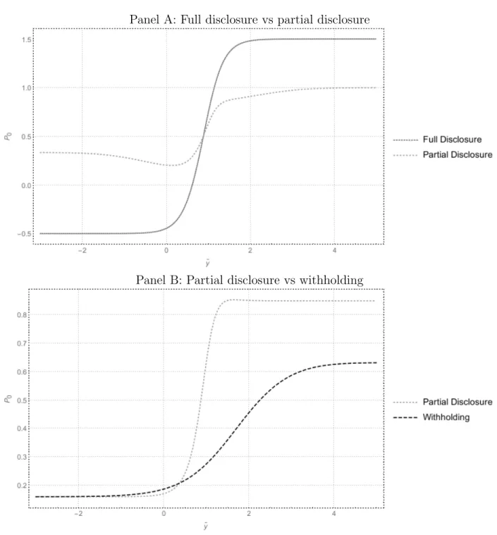
The method to obtain the manager’s optimal action is illustrated in two steps in Figure 1.2. Panel A shows the first part of the manager’s optimization problem: Given that investors know that the manager has an incentive to withhold information and that the manager has the option to use a second channel which unsophisticated investors cannot quickly process, what information should the manager disclose through the easy channel? In Panel A, the crossing of the full disclosure and partial disclosure lines indicates the value of the signal at which the manager is indifferent between partial and full disclosure. In this example, that cutoff is at 0.8825 – between the mean value of the good and bad firm. Once this cutoff is determined, the cutoff between partial disclosure and withholding can be determined, which is illustrated in Panel B of Figure 1.2. In Panel B, the intersection of the two lines again

(25)

indicates the point at which the manager would be indifferent between partial disclosure and withholding. This occurs at 0.3678. Note that while the graphs appear to converge on the left side, they are not quite equal – withholding leads to a higher price for all cutoffs less than the optimal cutoff, though the two lines limit to the same value.

In this numerical example, if the manager only had one channel available, a cutoff of 0.7535 would be optimal. Consistent with Corollary 2.1, the inclusion of a second channel leads to a decrease in the information available through the easy channel. Likewise, the inclusion of a second channel leads the manager to release more information to the market overall.

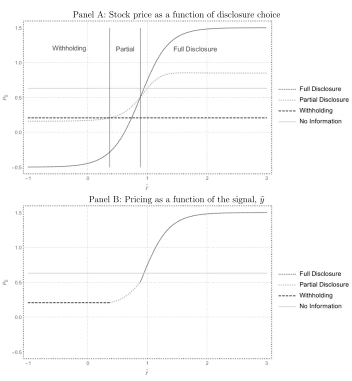
Figure 1.3 depicts how these disclosure choices impact the firm’s stock price. In Panel A, the stock price under each of the three disclosure strategies (along with the no information case) are presented for each level of the signal ˜𝑦. The points of indifference discussed above, 𝑐𝐹 𝐷 and 𝑐𝑃 𝐷, are included as solid vertical lines. As the price determined by withholding is

formed purely based on expectations derived from the endogenously determined cutoffs, the price is constant with respect to the value of the signal. On the far left, this constant value dominates the price that would be obtained through any type of disclosure. For middle values of the signal, the price from partial and full disclosure increases at a rapid rate. As the uninformed investors’ risk-adjusted expectation of firm value is higher than that of the informed investors, partial disclosure leads to a higher overall price in this region. On the right portion of the graph, the price from full disclosure dominates, as the signal is sufficiently high enough to raise the uninformed investor’s risk-adjusted expected value of the firm compared to the no disclosure case for them. In particular, when no disclosure is visible to the uninformed investors, they endogenously determine a 38.5% chance that the firm is good. Likewise, the rightmost cutoff occurs when full disclosure leads to a 38.5% probability that the firm is good.

(26)

1.5.2

Simulation

In order to understand how changes in the model parameters affect stock price and disclosure behavior in the model, 10,000 iterations of the model were run. Distributions for model parameters were chosen such that they always satisfy Theorem 1; the distributions are presented in Table 1.1. Parameters were chosen to represent a wide variety of values and for tractability. The probability of the manager acquiring the signal is allowed to vary from 0 to 1, encompassing all possible values. The number of investors, 𝑁, is fixed at 100 for simplicity in applying a distribution to the number of shares available, ¯𝑥, as the ratio of these quantities drives the effect of ¯𝑥. ¯𝑥 is allowed to vary between 50 and 100 shares, at integer values only. The number of uninformed investors is allowed to vary across the entire range from 1 to 𝑁 −1, guaranteeing that there is at least one of each investor type. The coefficient of risk aversion, 𝑎, is allowed to vary between 0 and 1, as that level covers a large amount of empirically identified risk aversion levels (see Table 1 of Babcock, Choi & Feinerman (1993)). The percentage chance that the firm is good is chosen to be between 0 and 0.5 for tractability in the simulation. The probability that the firm is good heavily influences the slope of the stock price, 𝑃0, with respect to the signal ˜𝑦, making the slopes at

the indifference points between disclosure choices more similar as 𝑝𝐺 increases. As such, the

numerical solver employed converges at a much faster rate when 𝑝𝐺 < 0.50. The standard

deviation, 𝜎 is bounded between 0.5 and 1, while 𝜇𝐺 is bounded between 1 and 3, and 𝜇𝐵

is set to 0. These choices assure that the condition of Theorem 1 is fulfilled and allow 𝜇𝐺 to

vary between 1 and 6 standard deviations above 𝜇𝐵.

1.5.3

Proof verification

One unique utility maximizing solution is found for the manager in each of the 10,000 it-erations of the simulation. This provides evidence that the equilibrium described in Theorem 2 is unique. Furthermore, it is noteworthy that of the 10,000 iterations, the unconditional expected stock price was higher in the two channel model than in the one channel model over 95% of the time, exactly 9,564 times. Furthermore, the unconditional expected firm price

(27)

was 0.0019 higher, on average, in the two channel case. Regarding the amount of information disclosed, the two channel case led to less disclosure in the easy channel in all iterations, though more information was disclosed overall in all iterations. Again, this is consistent with Corollary 2.1.

Furthermore, across all 9,913 iterations where equation (1.3) of Theorem 4 holds, 𝑃0 is

monotonic in both the full and partial disclosure states. In fact, 𝑃0 is monotonic over all

10,000 iterations in the partial disclosure state, whereas𝑃0 in the full disclosure state shows

some lack of monotonicity when the condition is not met (62 of 87 are not monotonic). Thus, the condition appears sufficient, though not necessary.

1.5.4

Statics

In order to understand how the unconditional stock price and disclosure pattern change with respect to the various parameters of the model, the simulation is necessary. In par-ticular, maximizing over the disclosure options leads to a maximization problem in which the main determinant, ˜𝑦 is contained in both the PDF and CDF of the normal distribution, leading to a seemingly intractable maximization problem. Through simulation, this issue can be addressed by varying the underlying parameters.

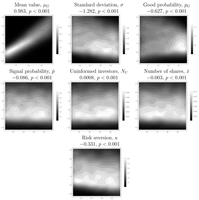
Figure 1.4 illustrates how the unconditional expected stock price varies with each of 7 parameters. As expected, increasing the mean of the distribution of good firm value increases the expected price, since that directly increases the investors expectation of firm value. Likewise, increasing the standard deviation leads to a decrease in stock price, as the investors are risk averse. Surprisingly, as the probability that the firm is good increases, the expected firm price decreases. Increasing the probability the firm is good has two main effects. First, the firm is more likely to be good, and thus the expected value of the firm will be higher. Second, increasing𝑝𝐺 will, over certain ranges, lead to an increase in the perceived volatility

of the firm. On average, it appears that the volatility effects overwhelm the mean effects (for 𝑝𝐺 < 0.5). Similarly, increasing the probability that the manager receives the signal

(28)

the number of uninformed investors leads to a small positive effect, driven by the larger information asymmetry between uninformed investors and the manager when compared to informed investors and the manager. Unsurprisingly, increasing the number of shares has a slight negative effect on the firm price, as the number of shares only enters into the firm pricing in a negative manner (see Proposition 2). Lastly, firm price decreases as the level of risk aversion among the investors rises, since investors will need to be compensated more for the risk they take on by investing.

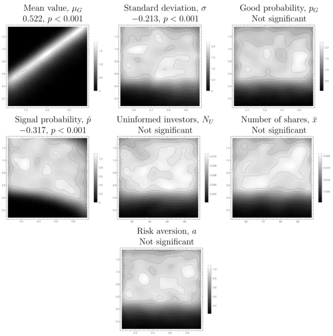
Regarding the effects of the model parameters on the manager’s disclosure choices, Figure 1.5 illustrates the effects on the cutoff between full disclosure and partial disclosure, while Figure 1.6 illustrates the effects on the cutoff between partial disclosure and withholding. Increasing the mean value of the good firm leads to higher levels for both cutoffs.6 _{This is}

due to the wider spread between the good and bad firms. Increasing the standard deviation has the opposite effect, leading the manager to disclose more fully and to lower the cutoff between partial disclosure and withholding. While the remaining factors do not exhibit a clear pattern for the lower cutoff, the probability that the manager receives a signal does appear to affect the cutoff between full and partial disclosure. As the probability the manager receives a signal increases, the manager appears to disclose more through the easy channel. The manager has an incentive to do this, as disclosing more makes uninformed investors believe that a lack of disclosure will be more likely caused by the manager not receiving the signal. The cutoff between partial and full disclosure is unaffected, as the informed investors will know whether or not the manager received a signal, regardless of the probability.

1.6

Empirical implications and conclusion

The primary model of this paper demonstrates the manager’s disclosure incentives when the manager has two voluntary disclosure channels in the presence of both uninformed and informed investors. The model follows a market for lemons structure in which the firm may be good or bad, and the manager probabilistically receives a signal that is potentially useful

(29)

in determining the firm’s type. If the manager receives a signal, the manager can choose to disclose through an easy-to-process channel, a hard-to-process channel, or no channel. When there is sufficient difference between the firm types, and when both informed and uninformed investors are present, the manager will adopt a three part disclosure strategy. For high values of the signal, the manager will disclose the signal through the easy-to-process channel. For low values of the signal, the manager will choose to not disclose, withholding the information from the market. If the value of the signal is in the middle, the manager will disclose through the hard-to-process channel.

This disclosure pattern is also consistent with maximizing the long-run stock price of the firm. The derived rational expectations equilibrium shows that the manager’s optimal actions are identical when maximizing the short-run and long-run stock prices. Furthermore, when the manager has two disclosure channels available, the stock price will be higher immediately after any optimal manager action excluding full disclosure than after the price has settled after multiple periods. Taken together, this indicates that, given any short run incentive to increase the stock price, the manager in this setting can costlessly capture a gain through the use of multiple disclosure channels.

The model further demonstrates that the manager will decrease disclosure to uninformed investors when given the option of disclosing via a secondary channel, though the manager will disclose more to the market overall. This could indicate a possible short-run inefficiency in the market as the uninformed investors learn the information disclosed through the sec-ondary voluntary channel. From the simulation, it appears that this short run effect could be priced, and would be driven by uninformed investors valuing the firm at a higher price than they would if they had processed all available information. However, the model also indicates that multiple channels of disclosure may serve to make the market more efficient over longer periods of time, as the market should fully impound more information than under a one disclosure channel system. As managers have the option to disclose through multiple sources, it is an open empirical issue 1) if and how managers use these channels in different

(30)

ways and 2) if disclosing differently across channels leads to an impact on the market.

1.7

Proofs

1.7.1

Existence

Proof. To establish existence of an non-degenerate equilibrium, there must exist some point 𝑦1 such that 𝑃0,𝐹 𝐷 > 𝑃0,𝑃 𝐷 and 𝑃0,𝐹 𝐷 > 𝑃0,𝑊 for all ˜𝑦 > 𝑦1, and some point 𝑦2 such that

𝑃0,𝐹 𝐷 < 𝑃0,𝑃 𝐷and𝑃0,𝐹 𝐷 < 𝑃0,𝑊 for all ˜𝑦 < 𝑦2. These conditions can be approached through

a limit argument.

First, let ˜𝑦, 𝑐𝐹 𝐷, 𝑐𝑃 𝐷 → ∞. Then 𝑝𝐼,𝐹 𝐷 = 𝑝𝑈,𝐹 𝐷 = 𝑝𝐼,𝑃 𝐷 → 1, as, for all 𝛿 > 0,

lim𝑥→∞_𝜑₍_𝑥₎₊𝜑(_𝜑𝑥₍)_𝑥₋_𝛿₎ = 1. Furthermore, 𝑝𝐼,𝑊, 𝑝𝑈,𝑃 𝐷, and 𝑝𝑈,𝑊 will all approach 𝑝𝐺, the

un-conditional probability that the firm is good, as, for all 𝛿finite, lim𝑥→∞ _Φ(_𝑥_)+Φ(Φ(𝑥)_𝑥₋_𝛿₎ = 1. Let 𝑝′ = 2𝑝𝐺2−2𝑝𝐺+ 1. Substituting these probabilities into the time 0 price expressions derived

in Section 1.7.2 yields: 𝑃0,𝐹 𝐷 > 𝑃0,𝑃 𝐷 as ˜𝑦, 𝑐𝐹 𝐷, 𝑐𝑃 𝐷 → ∞, ⇒ 1 𝑅𝑓 [︁ 𝜇𝐺−𝑎 ¯ 𝑥 𝑁𝜎 2]︁_> 𝑁𝐼𝜇𝐺+𝑁𝑈 𝑝𝐺𝜇𝐺+(1−𝑝𝐺)𝜇𝐵 2𝑝𝐺2−2𝑝𝐺+1 −𝑎𝑥𝜎¯ 2 𝑅𝑓 [︁ 𝑁𝐼+₂_𝑝 𝑁𝑈 𝐺2−2𝑝𝐺+1 ]︁ , ⇒ 𝜇𝐺 (︃ 1−𝑁𝐼 + 𝑝𝐺𝑁𝑈 𝑝′ 𝑁𝐼+ 𝑁_𝑝𝑈′ )︃ > 𝑁𝑈 (1−𝑝𝐺)𝜇𝐵 𝑝′ 𝑁𝐼+ 𝑁_𝑝𝑈′ +𝑎𝑥𝜎¯ 2 (︃ 1 𝑁 − 1 𝑁𝐼+ 𝑁_𝑝𝑈′ )︃ , ⇒ 𝑁𝑈(1−𝑝𝐺) 𝑁𝐼𝑝′+𝑁𝑈 𝜇𝐻 > 𝑁𝑈(1−𝑝𝐺) 𝑁𝐼𝑝′+𝑁𝑈 𝜇𝐿+𝑎𝑥𝜎¯ 2 𝑁𝑈(1−𝑝′) 𝑁(𝑁𝐼𝑝′+𝑁𝑈) , ⇒ 𝑁𝑈(1−𝑝𝐺) 𝑁𝐼𝑝′+𝑁𝑈 (𝜇𝐻 −𝜇𝐿)> 𝑎𝑥𝜎¯ 2 2𝑁𝑈𝑝𝐺(1−𝑝𝐺) 𝑁(𝑁𝐼𝑝′+𝑁𝑈) , ⇒ 𝜇𝐻 −𝜇𝐿>2𝑝𝐺𝑎 ¯ 𝑥 𝑁𝜎 2_. 𝑃0,𝐹 𝐷 > 𝑃0,𝑊 as ˜𝑦, 𝑐𝐹 𝐷, 𝑐𝑃 𝐷 → ∞, ⇒ 1 𝑅𝑓 [︁ 𝜇𝐺−𝑎 ¯ 𝑥 𝑁𝜎 2]︁_> 𝑁𝐼 𝑝𝐺𝜇𝐺+(1−𝑝𝐺)𝜇𝐵 2𝑝𝐺2−2𝑝𝐺+1 +𝑁𝑈 𝑝𝐺𝜇𝐺+(1−𝑝𝐺)𝜇𝐵 2𝑝𝐺2−2𝑝𝐺+1 −𝑎𝑥𝜎¯ 2 𝑅𝑓 [︁ 𝑁𝐼 2𝑝𝐺2−2𝑝𝐺+1 + 𝑁𝑈 2𝑝𝐺2−2𝑝𝐺+1 ]︁ ,

(31)

⇒ 𝜇𝐺−𝑎𝜎2 ¯ 𝑥 𝑁 > 𝑝𝐺𝜇𝐺+ (1−𝑝𝐺)𝜇𝐵−𝑎𝑝 ′ 𝜎2 𝑥¯ 𝑁, ⇒ (1−𝑝𝐺)(𝜇𝐺−𝜇𝐵)> 𝑎𝜎2 ¯ 𝑥 𝑁(2𝑝𝐺(1−𝑝𝐺)), ⇒ 𝜇𝐻 −𝜇𝐿>2𝑝𝐺𝑎 ¯ 𝑥 𝑁𝜎 2_.

Both conditions are identical, requiring that the difference between the mean of the distribution for 𝑃1 for the good firm and bad firm be above a threshold of 2𝑝𝐺𝑎_𝑁𝑥¯𝜎2.

Next, ˜𝑦, 𝑐𝐹 𝐷, 𝑐𝑃 𝐷 → −∞. Under this limit, 𝑝𝐼,𝐹 𝐷 = 𝑝𝑈,𝐹 𝐷 = 𝑝𝐼,𝑃 𝐷 = 𝑝𝐼,𝑊 → 0, and 𝑝𝑈,𝑃 𝐷 =𝑝𝑈,𝑊 →𝑝𝐺. Let 𝑝′ = 2𝑝𝐺2−2𝑝𝐺+ 1. Substituting these probabilities into the time

0 price expressions derived in Section 1.7.2 yields:

lim 𝑐→−∞𝑃0,𝐹 𝐷 = 1 𝑅𝑓 [︁ 𝜇𝐵−𝑎 ¯ 𝑥 𝑁𝜎 2]︁_, lim 𝑐→−∞𝑃0,𝑃 𝐷 = 𝑁𝐼𝜇_𝜎𝐵2 +𝑁𝑈 𝑝𝐻𝜇𝐺+(1−𝑝𝐻)𝜇𝐵 𝑝′_𝜎2 +𝑎𝑥¯ 𝑅𝑓 (︁ 𝑁𝐼 𝜎2 + 𝑁𝑈 𝑝′_𝜎2 )︁ , lim 𝑐→−∞𝑃0,𝑊 = 𝑁𝐼𝜇_𝜎𝐵2 +𝑁𝑈𝑝𝐻𝜇𝐺+(1 −𝑝𝐻)𝜇𝐵 𝑝′_𝜎2 +𝑎𝑥¯ 𝑅𝑓 (︁ 𝑁𝐼 𝜎2 + 𝑁𝑈 𝑝′_𝜎2 )︁ .

Note that the limits for 𝑃0,𝑃 𝐷 and 𝑃0,𝑊 are the same. Thus, if, in the limit, 𝑃0,𝐹 𝐷 < 𝑃𝑃 𝐷,

then 𝑃0,𝐹 𝐷< 𝑃0,𝑊. 1 𝑅𝑓 [︁ 𝜇𝐵−𝑎 ¯ 𝑥 𝑁𝜎 2]︁_< 𝑁𝐼 𝜇𝐵 𝜎2 +𝑁𝑈𝑝𝐻𝜇𝐺+(1 −𝑝𝐻)𝜇𝐵 𝑝′_𝜎2 +𝑎𝑥¯ 𝑅𝑓 (︁ 𝑁𝐼 𝜎2 + 𝑁𝑈 𝑝′_𝜎2 )︁ , ⇒ 𝑁𝑈 𝑝′_𝜎2𝜇𝐵−𝑎𝑥¯ (︂ 𝑁𝐼 𝑁 + 𝑁𝑈 𝑁 𝑝′ )︂ < 𝑁𝑈𝑝𝐺 𝑝′_𝜎2 𝜇𝐺+ 𝑁𝑈(1−𝑝𝐺) 𝑝′_𝜎2 𝜇𝐵−𝑎𝑥,¯ ⇒ − 𝑁𝑈𝑝𝐺 𝑝′_𝜎2 (𝜇𝐺−𝜇𝐵)< 𝑎𝑥¯ 𝑁𝑈 𝑁 𝑝′(1−𝑝 ′ ).

Since 𝜇𝐺 > 𝜇𝐵 by definition and since 𝑝′ ∈ (0.5,1), the statement holds for all parameter

values.

(32)

solution exists.

1.7.2

Derivation

This section derives 𝑃0 under each of the four states: full disclosure, partial disclosure,

withholding, and no information.

First, the probabilities in Lemma 1 must be derived. Per Bayes’ theorem, _P(𝐴|𝐵) = P(𝐴)P(𝐵|𝐴)

P(𝐵) , and P(𝐵) =P(𝐴)P(𝐵|𝐴) +P

(︀

𝐴{)︀_P(︀𝐵|𝐴{)︀.

Furthermore, note that under full disclosure, both investor types know ˜𝑦. Under par-tial disclosure, the informed investors will likewise know ˜𝑦. Under withholding, informed investors know that ˜𝑦 < 𝑐𝑃 𝐷, where 𝑐𝑃 𝐷 is an endogenously determined cutoff. Under no

information, informed investors are aware that the manager did not receive a signal, and thus have no information to condition on. For uninformed investors, if the state is not full disclosure, they cannot determine the state. As such, they must endogenously determine probabilities based on a cutoff 𝑐𝐹 𝐷 below which full disclosure will not occur. Thus, for

investor 𝑖 and state 𝑠, the conditional probability that the firm is good conditioned on the given information can be defined as 𝑝𝑖,𝑠. Let 𝛽𝑥,𝑇 = 𝑥−_𝜎𝜇𝑇, 𝜑(𝑥) be the normal distribution

PDF, and Φ(𝑥) be the normal distribution CDF.

1. It is easy to see that 𝑝𝐼,𝑁 𝐼 =𝑝𝐺, as this is the unconditional probability that the firm

is good. 2. _P(˜𝑦 < 𝑐|𝑇) = Φ(︀𝑐−𝜇𝑇 𝜎 )︀ = Φ (𝛽𝑐,𝑇). Thus, 𝑝𝐼,𝑊 = 𝑝𝐺Φ(𝛽_{𝑐𝑃 𝐷,𝐺}) 𝑝𝐺Φ(𝛽_{𝑐𝑃 𝐷,𝐺})+(1−𝑝𝐺)Φ(𝛽_{𝑐𝑃 𝐷,𝐵}). 3. Likewise, _P(˜𝑦 < 𝑐 or _@𝑦˜|𝑇) = ˆ𝑝Φ(𝛽𝑐𝐹 𝐷,𝐺) + (1−𝑝ˆ). Thus, 𝑝𝑈,𝑃 𝐷 = 𝑝𝑈,𝑊 = 𝑝𝑈,𝑃 = 𝑝𝐺(𝑝^Φ(𝛽_{𝑐𝐹 𝐷,𝐺})+(1−𝑝^)) ^ 𝑝₍𝑝𝐺Φ(𝛽_{𝑐𝐹 𝐷,𝐺})+(1−𝑝𝐺)Φ(𝛽_{𝑐𝐹 𝐷,𝐵}))+(1−𝑝^).

4. When a specific ˜𝑦 is known, applying Bayes’ theorem is trickier, as direct application would lead to using _P(𝑦=𝑐|𝑇) = 0. However, this is simply a case of working in a continuous case. In the discrete case, it is intuitive to see that the problem would result

(33)

in a ratio of PDFs of the underlying distribution. This is the same for the continuous case. Thus,𝑝𝐼,𝐹 𝐷 =𝑝𝐼,𝑃 𝐷 =𝑝𝑈,𝐹 𝐷 =

𝑝𝐺𝜑(𝛽𝑦,𝐺)

𝑝𝐺𝜑(𝛽𝑦,𝐺)+(1−𝑝𝐺)𝜑(𝛽𝑦,𝐵).

Thus, the derivation of Lemma 1 is complete. Next, using equation (1.2) the price can be derived under a general state. From (1.2),

𝑥𝑖,𝑠= E [︁ ˜ 𝑃1|𝐼𝑖,𝑠 ]︁ −𝑅𝑓𝑃0 𝑎_V [︁ ˜ 𝑃1|𝐼𝑖,𝑠 ]︁ . Aggregating 𝑥𝑖,𝑠 up to ¯𝑥: ¯ 𝑥=𝑁𝐼𝑥𝐼,𝑠+𝑁𝑈𝑥𝑈,𝑠.

Solving the above for 𝑃0,𝑠 yields:

Next, this expression can be explicitly provided for each of the four states. Note that

E [︁ ˜ 𝑃1|𝐼𝑖,𝑠 ]︁ =𝑝𝑖,𝑠𝜇𝐺+(1−𝑝𝑖,𝑠)𝜇𝐵 andV [︁ ˜ 𝑃1|𝐼𝑖,𝑠 ]︁ =𝑝𝑖,𝑠2𝜎2+(1−𝑝𝑖,𝑠)2𝜎2 = (2𝑝𝑖,𝑠2−2𝑝𝑖,𝑠+1)𝜎2.

Thus, the price at time 0 can explicitly be written, under each of the four states, as:

𝑃0,𝐹 𝐷= 1 𝑅𝑓 [︁ 𝑝𝐼,𝐹 𝐷𝜇𝐺+ (1−𝑝𝐼,𝐹 𝐷)𝜇𝐵−𝑎 ¯ 𝑥 𝑁(2𝑝𝐼,𝐹 𝐷 2₋₂_𝑝 𝐼,𝐹 𝐷 + 1)𝜎2 ]︁ , 𝑃0,𝑃 𝐷= 𝑁𝐼 𝑝𝐼,𝐹 𝐷𝜇𝐺+(1−𝑝𝐼,𝐹 𝐷)𝜇𝐵 2𝑝𝐼,𝐹 𝐷2−2𝑝𝐼,𝐹 𝐷+1 +𝑁𝑈 𝑝𝑈,𝑊𝜇𝐺+(1−𝑝𝑈,𝑊)𝜇𝐵 2𝑝𝑈,𝑊2−2𝑝𝑈,𝑊+1 −𝑎𝑥𝜎¯ 2 𝑅𝑓 [︁ 𝑁𝐼 2𝑝𝐼,𝐹 𝐷2−2𝑝𝐼,𝐹 𝐷+1 + 𝑁𝑈 2𝑝𝑈,𝑊2−2𝑝𝑈,𝑊+1 ]︁ , 𝑃0,𝑊 = 𝑁𝐼 𝑝𝐼,𝑊𝜇𝐺+(1−𝑝𝐼,𝑊)𝜇𝐵 2𝑝𝐼,𝑊2−2𝑝𝐼,𝑊+1 +𝑁𝑈 𝑝𝑈,𝑊𝜇𝐺+(1−𝑝𝑈,𝑊)𝜇𝐵 2𝑝𝑈,𝑊2−2𝑝𝑈,𝑊+1 −𝑎𝑥𝜎¯ 2 𝑅𝑓 [︁ 𝑁𝐼 2𝑝𝐼,𝑊2−2𝑝𝐼,𝑊+1 + 𝑁𝑈 2𝑝𝑈,𝑊2−2𝑝𝑈,𝑊+1 ]︁ , 𝑃0,𝑁 𝐼 = 𝑁𝐼𝑝𝐺𝜇𝐺+(1 −𝑝𝐺)𝜇𝐵 2𝑝𝐺2−2𝑝𝐺+1 +𝑁𝑈 𝑝𝑈,𝑊𝜇𝐺+(1−𝑝𝑈,𝑊)𝜇𝐵 2𝑝𝑈,𝑊2−2𝑝𝑈,𝑊+1 −𝑎𝑥𝜎¯ 2 𝑅𝑓 [︁ 𝑁𝐼 2𝑝𝐺2−2𝑝𝐺+1 + 𝑁𝑈 2𝑝𝑈,𝑊2−2𝑝𝑈,𝑊+1 ]︁ .

(34)

1.7.3

Disclosure patterns

Proof. From the proof of Theorem 1, as the two disclosure cutoffs and ˜𝑦 approach infinity, full disclosure will have a higher price than partial disclosure and withholding when the existence condition is met. Thus, full disclosure will be used for at least all ˜𝑦 above some point ¯𝑦. Furthermore, from the proof of Theorem 1, as the two disclosure cutoffs and ˜𝑦 approach negative infinity, full disclosure will have a lower price than partial disclosure and withholding. Thus, full disclosure will not be the only strategy employed.

Furthermore, note that 𝑝𝑈,𝑃 𝐷 is a monotonic function of the signal ˜𝑦, and ranges from

0 to 1. Likewise, 𝑝𝑈,𝑊 is a monotonic function of the cutoff between partial disclosure and

withholding, but ranges from 0 to𝑝𝐺. Thus, when the cutoff is at ˜𝑦, these two lines will cross

for some value ˜𝑦=𝑐𝑃 𝐷. Also note that𝑝𝑈,𝑃 𝐷, while not monotonic in the cutoff between full

disclosure and partial disclosure, is bounded above at 𝑝𝐺 and is bounded below by the value

of 𝑝𝐼,𝑃 𝐷, as 𝑝𝑈,𝑃 𝐷 represents a transformation of 𝑝𝐼,𝑃 𝐷 = 𝑁_𝐷 to𝑝𝑈,𝑃 𝐷 = 𝑓(𝑁, 𝐷) = 𝑎𝑁_𝑎𝐷+1₊₁₋−_𝑎𝑎,

where 𝑎, 𝐷, 𝑁 ∈(0,1). Thus, for some ˜𝑦=𝑐𝐹 𝐷, 𝑝𝑈,𝑃 𝐷 =𝑝𝐼,𝑃 𝐷 and 𝑐𝐹 𝐷 > 𝑐𝑃 𝐷.

Now, consider a specific case in which 𝑃0,𝐹 𝐷 = 𝑃0,𝑃 𝐷. Let ˜𝑦 be a signal such that 𝑝𝑈,𝐹 𝐷 = 𝑝𝑈,𝑃 𝐷. In this case, the inferred distributions by uninformed investors will be the

same regardless of the manager’s disclosure choice. This case occurs when ˜𝑦 = 𝑐𝐹 𝐷 as

discussed above, and thus exists.

Next, consider a specific case in which 𝑃0,𝑃 𝐷 = 𝑃0,𝑊. Let ˜𝑦 be the signal such that 𝑝𝐼,𝑃 𝐷 =𝑝𝐼,𝑊. In this case, the inferred distributions by informed investors will be the same

regardless of the manager’s disclosure choice. This case occurs when ˜𝑦 = 𝑐𝑃 𝐷 as discussed

above, and thus also exists. Furthermore, 𝑐𝑃 𝐷 is strictly less than𝑐𝐹 𝐷, and thus there exists

a bounded region on which the manager will prefer partial disclosure. Furthermore, below the boundary of the region, the manager will prefer withholding.

Thus, all three disclosure options will be used in the manager’s optimal disclosure strat-egy: withholding for low values of ˜𝑦, partial disclosure for middle values, and full disclosure

(35)

for high values.7

7_{Note that while this proof shows that the manager will have 2 cutoff points, it does not preclude the} manager from having cutoff points other than the 2 mentioned. Thus, it does not fully constitute a proof of uniqueness. Such a proof would need to show that no cutoff point can exist when the probability that the firm is good from the investors’ perspective changes based on the manager’s disclosure choice.

(36)

Figures

Figure 1.1: Diagram of the full model

Firm

Manager

Easy Channel

Hard Channel

Uninformed

Investors

Informed Investors

A diagram of the flow of information in the market. Solid lines represent information transfers, dashed lines represent partial information transfers, and dotted lines represent information transfers that only occur in the long run.

(37)

Figure 1.2: Optimizing disclosure

Panel A: Full disclosure vs partial disclosure

Panel B: Partial disclosure vs withholding

These two graphs illustrate the process for choosing the optimal disclosure cutoff points from the manager’s perspective. The graphs are based on the numerical example parameters listed in Table 1.1.

(38)

Figure 1.3: Optimal disclosure

Panel A: Stock price as a function of disclosure choice

Panel B: Pricing as a function of the signal, ˜𝑦

These graphs show the stock price at time 0, 𝑃0, as a function of the signal the manager receives (if received) and the manager’s disclosure choice. Panel A shows the payoffs for all disclosure choices, whereas Panel B shows the price as a function of the manager’s optimal choices. These graphs are based on the numerical example parameters listed in Table 1.1.

(39)

Figure 1.4: Pricing statics

Mean value,𝜇𝐺 Standard deviation,𝜎 Good probability, 𝑝𝐺

0.983, 𝑝 <0.001 −1.282, 𝑝 <0.001 −0.627, 𝑝 < 0.001

Signal probability, ˆ𝑝 Uninformed investors, 𝑁𝑈 Number of shares, ¯𝑥 −0.086, 𝑝 <0.001 0.0008, 𝑝 < 0.001 −0.003, 𝑝 < 0.001

Risk aversion,𝑎 −0.331, 𝑝 <0.001

These smoothed density histograms show the relationship between firm price at time 0 (𝑃0) on the vertical axes and various parameters of the model on the horizontal axes. These plots are based on a simulation of 10,000 iterations of the model (see Table 1.1 for specific details). Lighter colors represent a greater concentration of values near the specific parameter-price pairing, and the enclosed regions represent level curves of the density at 10% intervals. Significant trends based on OLS regressions are noted above the graphs; graphs with no significant trends are instead marked as such.

(40)

Figure 1.5: Disclosure statics, cutoff between full disclosure and partial disclosure

0.522, 𝑝 <0.001 −0.213, 𝑝 <0.001 Not significant

Signal probability, ˆ𝑝 Uninformed investors, 𝑁𝑈 Number of shares, ¯𝑥 −0.317, 𝑝 <0.001 Not significant Not significant

Risk aversion,𝑎 Not significant

These smoothed density histograms show the relationship between the disclosure cutoff between full disclosure and partial disclosure on the vertical axes and various parameters of the model on the horizontal axes. These plots are based on a simulation of 10,000 iterations of the model (see Table 1.1 for specific details). Lighter colors represent a greater concentration of values near the specific parameter-disclosure cutoff, and the enclosed regions represent level curves of the density at 10% intervals. Significant trends based on OLS regressions are noted above the graphs; graphs with no significant trends are instead marked as such.

(41)

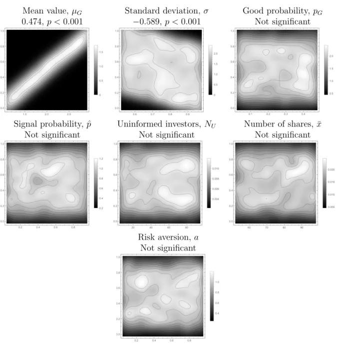
Figure 1.6: Disclosure statics, cutoff between partial disclosure and withholding

0.474, 𝑝 <0.001 −0.589, 𝑝 <0.001 Not significant

Signal probability, ˆ𝑝 Uninformed investors, 𝑁𝑈 Number of shares, ¯𝑥

Not significant Not significant Not significant

Risk aversion,𝑎 Not significant

These smoothed density histograms show the relationship between the disclosure cutoff between partial disclosure and withholding on the vertical axes and various parameters of the model on the horizontal axes. These plots are based on a simulation of 10,000 iterations of the model (see Table 1.1 for specific details). Lighter colors represent a greater concentration of values near the specific parameter-disclosure cutoff, and the enclosed regions represent level curves of the density at 10% intervals. Significant trends based on OLS regressions are noted above the graphs; graphs with no significant trends are instead marked as such.

(42)

Tables

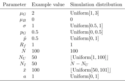
Table 1.1: Numerical example and simulation parameters

Parameter Example value Simulation distribution

𝜇𝐺 2 Uniform[1,3] 𝜇𝐵 0 0 𝜎 1 Uniform[0.5,1] 𝑝𝐺 0.5 Uniform[0,0.5] ^ 𝑝 0.5 Uniform[0,1] 𝑅𝑓 1 1 𝑁 100 100 𝑁𝑈 50 ⌊Uniform[1,100]⌋ 𝑁𝐼 50 𝑁−𝑁𝑈 ¯ 𝑥 100 ⌊Uniform[50,101]⌋ 𝑎 1 Uniform[0,1]

This table shows the distributions for each parameter in the simulation. The parameter choices are chosen such that 2𝑝𝐺𝜎2 ¯_𝑁𝑥 <1 and𝜇𝐺−𝜇𝐵>1, thus fulfilling the requirements of Corollary 1.

(43)

2 Market Reaction to Shifting of

Voluntary Disclosures Across

Disclosure Channels

2.1

Introduction

Managers are gatekeepers of information about their firms. Consequently, managerial incentives can shape how information is voluntarily disclosed by a firm. This paper explores a new way in which managers can shift voluntary disclosures: by choosing between two dis-closure channels based on the perceived ease or difficulty for users to process the information. I build a scenario around two disclosure channels taking on two opposing levels of ease of processing: easy or difficult to process. The basic premise is that managers more frequently choose the easy to process channel to communicate positive information and the difficult to process channel to communicate negative information. I operationalize this design by using the voluntary portion of SEC filings as the difficult to process channel and select portions of firm websites (excluding advertising, commerce pages, support pages, etc.) as the easy to process channel. I propose that these two channels