See discussions, stats, and author profiles for this publication at: https://www.researchgate.net/publication/270071672
Analysing wireless sensor network deployment performance using connectivity
Article in ScienceAsia · July 2013DOI: 10.2306/scienceasia1513-1874.2013.39S.080 CITATIONS 3 READS 9 3 authors, including:
Some of the authors of this publication are also working on these related projects:
pseudonym generation using palm vein in preserving data privacy for healthcare organizationView project
Red Blood CellView project Shukor Abd Razak
Universiti Teknologi Malaysia
133PUBLICATIONS 759CITATIONS
SEE PROFILE
Abdul Samad Ismail
Universiti Teknologi Malaysia
89PUBLICATIONS 587CITATIONS
SEE PROFILE
R
doi: 10.2306/scienceasia1513-1874.2013.39S.080
Analysing wireless sensor network deployment
performance using connectivity
Kamal Jadidy Aval∗, Shukor Abd Razak, Abdul Samad Ismail
Department of Computer Science, Faculty of Computing, Universiti Teknologi Malaysia, Johor, Malaysia ∗Corresponding author, e-mail: [email protected]
Received 7 Jan 2013 Accepted 5 Apr 2013
ABSTRACT: In contrast to the random deployment method for wireless sensor networks, there are various applications that require manual deployment. While the deployment is costly and usually there is no change in the position of the nodes, it is better to evaluate the deployment scheme before doing it. There are different existing metrics to evaluate a deployment including coverage, connectivity, network lifetime, and cost. With emerging real applications of WSNs, it has become a must to evaluate the deployments with more realistic metrics and model. In this paper we have proposed an accumulative path reliability rate metric, regarding the hop-based nature of routing in these networks, to measure the connectivity between two nodes that are not adjacent. We have applied the metric to existing deployment methods and analysed the results. KEYWORDS: WSN, shadowing effect, accumulative path reliability rate, manual deployment
INTRODUCTION
With the technological advances in MEMS (micro electro-mechanical systems)1, low powered ICs are being used in wireless sensor network (WSN) nodes. This has made the applications of WSNs commoner and closer to the real world scenarios. Every wireless sensor node is composed of a wireless transceiver, a processor, and at least one sensor2. The data is
collected from the environment and then carried to
sink nodes. The sink nodes process the data and
depending on the application send the commands to the actuators or fires alarms for human resources to take proper action. There may be one or more sink nodes in a whole WSN.
As the only energy resource of the nodes is a battery, there has been a lot of effort making the networks more durable. On the other hand, the real-time communication between nodes and especially from node to the sink has overridden the extension of the network lifetime2. At the same time, it is also important to be sure that the data sensed by a node will be delivered to the sink node successfully.
The quality of deployment in the WSNs applica-tion in the real world applicaapplica-tion has become more important than wired networks while the communica-tion is based on the impressionable wireless connec-tions. Researchers have introduced some connectivity models to allow qualification of the WSNs from the communication point of view. The quality assessment of a WSN can be useful in both random and manual
deployment of wireless sensor networks. After a ran-dom deployment of the nodes, which can be scattering from an aeroplane, a qualification can highlight the area with poor density of nodes to be improved by a second placement solution. On the other hand, in manual deployment the qualification of the deploy-ment can be done even before the deploydeploy-ment and help the designer to choose the best positions for the nodes of the network. In this paper we propose a communication qualification metric for WSNs.
As opposed to the existing connectivity metrics, this metric presents the expectancy of the delivery of data from where is sensed to where it is used for making the decision for an action. We assume that the application is large enough to have multi-hop communication between nodes. The remainder of this paper is organized as follows. The following section reviews the existing connectivity issues and models in the wireless area. Then the current work for qualification of wireless communication of the WSNs is presented. After that, accumulative path reliability rate is presented as the proposed metric for qualifica-tion of the WSNs. This is followed by analysis of the existing deployments using the proposed metric and presents a discussion.
WIRELESS CONNECTIVITY
As one of the main goals in WSN is to save electricity as much as it is possible, the communication between the nodes of the network is highly unreliable. Like any other physical phenomenon, there are models to
ScienceAsia39S (2013) 81 represent the phenomenon. Binary disc is the simplest
model so far. In this model every two sensor nodes in the terrain are connected if and only if their Euclidian distance is less than or equal to a predefined value. This communication range depends on the transmis-sion and reception power level of the nodes. If there are different transmission power levels in a network the minimum transmission power will be used. This model has proved to be far from the real behaviour of the radio links that are highly irregular3.
Another communication modelling method is as-suming the irregularity of the radio links and the fact that the received signal in the transceiver depends on the distance and the environment. According to this model the received signal power is calculated using
Pr= Ps d(si, sj)η
(1) wherePris the power of the received signal,Psis the power of the transmitted signal,η is the environment dependent path loss, and thed(si, sj)is the Euclidian
distance between two nodes. Using this model, a node is able to receive data when the Pr is more than a
predefined threshold.
As a complementary solution to the previous idea of attenuation, the existence of other nodes of the network has been used in the third model. This model takes the impact of the interference with other nodes of the network and the noise of the environment. The SINR model4uses a predefined threshold ofSINRθto
decide whether the data is received in the transceiver or not:
Pr(si)
N+P
sk∈χ\siPr(sk)
>SINRθ (2)
where N is the noise of the environment and χ is
the set of all nodes of the network. According to the SINR model, it is possible that two close nodes are not able to communicate just because of the interference provided by other adjacent nodes. It also becomes possible for two far nodes to communicate in the absence of interference and noise.
The log-normal shadowing model3 is another
common model which tries to consider all parameters that affect the received signal. The effect of multiple paths is given by
PL(d) = PL(d0) + 10ηlog10 d d0
+Xσ. (3) wherePL(d)is used to represent the signal strength loss at distancedfrom the sender,d0is the reference
distance, η is the path-loss exponent, and Xσ is a
zero-mean Gaussian random variable with standard deviation σ. The strength of the received signal at a distancedfrom a sender is its transmission power minusPL(d). Curve fitting of experimental data is used to obtain σ. PL(d0) can either be calculated
using analysis or obtained by conducting experiments. RELATED WORK
The nature of the wireless sensor network forces the hop by hop routing schemes. Although some routing techniques consider quality of the packet delivery for choosing links after deployment5, there is no such
metric in manual deployment cases to evaluate the deployment plan. Unreliability has a great impact on the quality of the communication through the network. The remainder of this section reviews the existing work on the quality of communication in terms of rate of successful packet delivery.
In Ref. 3, the authors have conducted various experiments to present a more realistic mathematical model of the node communication. There has been a comprehensive analysis of the basic parameters in unreliability and asymmetry. There are expressions for variance, distribution, and expectation of the packet reception rate in terms of the Euclidian distance between network nodes. They have analysed the be-haviour of the communication links in the transitional or grey region.
The authors of Ref.6have introduced a new MAC protocol and have done many experiments to study the behaviour of the physical layer. According to their simulations and experiments, they have defined a new metric to measure the quality of the communication link between two nodes as the probability of success-fully receiving (PSR) a packet:
p(d) = 1−1 2exp −SNR(d) 1.28 !8f (4)
where d is the distance and f is the packet size in bytes.
The authors of Ref. 7 have conducted empirical simulations and analysed the distribution, indepen-dence, and the temporal properties of the received sig-nal strength and the rate of error. The results show that the studied properties vary according to the operating zone and are similar for the same category. Packet error rate is the metric they have used to measure the quality of a link. In a similar study, researchers in
Ref. 8 have conducted some experiments using the
CC2420 from Chipcon. They have tested the nodes both in outdoor and indoor environment to measure the packet reception rate that indicated the rate of
correctly received packets. They have also studied the bit error rate both analytically and experimentally. ACCUMULATIVE PATH RELIABILITY RATE In this section we discuss a model of the new metric to rate path reliability.
Model
The model proposed in Ref. 3 is used as the base
idea of existence and behaviour of transitional region. The model considers all of the parameters affecting the wireless communication. Path loss exponent (n) and shadowing variance (σ2) are the
environment-dependent parameters. For example, the path loss
exponent of a parking structure is 3.0 while it is 2.0 for an apartment hallway9. These parameters either must be obtained through experiments or used from published results9. The SNR(signal-to-noise ratio)
depends on the hardware used for wireless communi-cation. The use of various modulations (ASK, FSK, and PSK) affects the quality of the communication
too. The effect of the exploited encoding is also
considered in this general model. Based on the above model and the assumptions made in Ref.5we will use (4).
Metric
The hop-by-hop nature of the peer-to-peer wireless sensor networks leads to the propagation of the com-munication quality factors. After a packet is initiated in a node and is on its way to the destination (normally sink node) the quality of each wireless link between two nodes on the path affects the overall quality of the delivery. Using packet reception rate to indicate the probability of successful delivery of the packets from one node to the next node in the path, and accumulating these rates according to the location of the nodes in the network, the accumulative path reliability rate APRR is defined as the probability of successful delivery of a packet from source to destination through a hop-by-hop route. This metric can be simply calculated by multiplication of the packet reception rate all over the route from source node to the destination node.
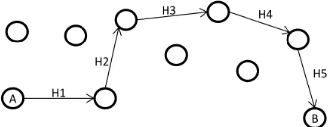
Consider one packet originating from node A and taking five hops of H1–H5 on its way to the destination node B. Fig. 1 illustrates an example of hop-by-hop routing in a wireless sensor network. The distance between the nodes of the route is considered as roughly constant. The roughly constant distance between the nodes will result in an almost constant packet reception rate that is considered to be 90%.
A B H1 H2 H3 H4 H5
Fig. 1 An example of hop by hop routing.
The accumulative path reliability rate for the route shown inFig. 1is given by
APRRH1−H5
= PRRH1PRRH2PRRH3PRRH4PRRH5. (5)
In the above example, if we calculate theAPRRfor the route from A to B, the probability of successfully delivering a packet from A to B will be (90%)5, that is, 59%. Although the minimum quality of commu-nication between any connected pair of nodes in the route is 90%, the probability of successful delivery of a packet through a route of five hops becomes
less than 60%. In case of manual deployment of
nodes, this metric will become useful for evaluating and comparing different strategies for its minimum, average, and standard deviation of all possible routes of the network. Major existing deployment strategies will be discussed and analysed next.
ANALYSIS AND DISCUSSION
Whenever predetermined node locations are used to deploy a wireless sensor network, it becomes possible to evaluate some of the characteristics of the net-work and do any possible improvement before actual
deployment. The APRR is one of the metrics to
evaluate a deployment strategy. The metric can only be applied to the strategies using this model. In the following, two cases of regular deployment and non-regular deployments and the simulation results will be discussed.
Regular deployment
In the case of regular deployments, as it can be seen in Fig. 2, the distance between every two node is constant that results in a constant rate ofPRR. This in turn leads to an exponential dependence between
maximum APRR and PRR at a power of terrain
diameter in terms of hop count.
In the examples illustrated inFig. 2, two possible cases of regular deployment are shown.Fig. 2a shows a deployment without any sink node defined. In this
ScienceAsia39S (2013) 83
(a)
(b)
Fig. 2 Regular deployment (a) without and (b) with sink node (the black node).
example the longest path consists of 19 hops. In this case
APRR = (PRR)19. (6)
According to this and assuming APRRmin as the
minimumAPRRthat the network can tolerate,
PRRmin= 19
p
APRRmin. (7)
Using this parameter, the transmission power of the network nodes must be adjusted to a value that can
provide PRRmin. As an alternative solution, the
number of nodes must be increased to provide a denser network with closer nodes. As with the case inFig. 2a, the terrain illustrated inFig. 2b represents a regularly deployed network. In this case, all the nodes send their data to the sink node and it is very easy to calculate the maximum and average number of hops as the distance of each node in the network from the sink node. There are 6, 12, 18, 24, 18, 18, 18, 15, 8, 2 nodes, respectively, within 1, 2, 3, 4, 5, 6, 7, 8, 9, 10 hops distance of the sink node. In this case the weighted average is 5.15 which means the weighted average ofAPRRwill bePRR5.15taking the number of nodes in each class as the weight. The maximum number of hops is 24 and accordingly the maximum
number ofAPRRwill be(PRR)24.
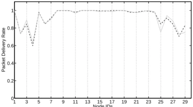
1 3 5 7 9 11 13 15 17 19 21 23 25 27 29 0 0.2 0.4 0.6 0.8 1 Node IDs
Packet Delivery Rate
Fig. 3 Theoretical and simulated accumulative path reli-ability rate. Grey line: simulated APRR; dashed line: theoreticalAPPR.
Non-regular deployment
In other deployment methods,APRR could be used
to either provide a more suitable node position in the deployment or assess results of a deployment (even a
random one). In this case theAPRR values cannot
be calculated as simply as the deployment example shown in Fig. 2b. To do this, all the routes of the
network must be discovered and then the PRR for
each hop of the route will be used to calculateAPRR. The solutions based on evolutionary algorithms10–13
can use this metric to evaluate the resulting deploy-ment in each step of their algorithms. The solutions may also be modified by using this metric to improve the evolution of the result set in the iterations of the algorithms.
Simulation results
To make sure that (5) complies with the real world deployment scenarios, we have conducted some sim-ulations using MATLAB. In this simulation we have assumed the routing to be simple AODV and all of the nodes send their sensed data to the sink node which is located at the centre of the terrain. Fig. 3 shows the results for a random data flow from network nodes towards the sink node. It can be seen that for nodes 12,
21, and 23,APRRis below 80% which means only
80% of the sensed data will arrive at the sink node. Once the simulation time is increased the differences between the theoretical and simulation results will become even less.
CONCLUSIONS AND FUTURE WORK
A deployment of wireless sensor network must meet the minimum requirements of quality factors to be
successful. Common WSN metrics to evaluate a
deployment are coverage, connectivity, cost, and life-time. Although the hop-by-hop routing is an intrinsic
property of these networks, the effect of this type of routing on the quality of packet delivery throughout
the network is not considered. In this paper we
proposed a metric to evaluate the probability of packet delivery between network nodes. This metric could be used in deployment solutions to prevent unreliable communication over long routes. Without consider-ing this metric, there is no difference between two connected network deployments. Our metric can help designers to rank two or more connected networks in terms of quality of data delivery.
We are going to extend our research in two ar-eas. Firstly we will apply this metric on the existing solutions for deployment to provide an analytical comparison. Secondly, we will use this metric in a solution with an evolutionary algorithm to refine the resulting network map.
Acknowledgements: This study was supported by
MOHE, Malaysia.
REFERENCES
1. Teymoori M, Abbaspour-Sani E (2002) A novel elec-trostatic micromachined pump for drug delivery sys-tems. In: IEEE International Conference on Semicon-ductor Electronics, pp 105–9.
2. Boughanmi N, Song Y (2008) A new routing metric for satisfying both energy and delay constraints in wireless sensor networks.J Signal Process Syst51, 137–43. 3. Zuniga M, Krishnamachari B (2004) Analyzing the
transitional region in low power wireless links. In:First Annual IEEE Communications Society Conference on Sensor and Ad Hoc Communications and Networks, pp 517–26.
4. Dousse O, Baccelli F, Thiran P (2005) Impact of interferences on connectivity in ad hoc networks.
IEEE/ACM Trans Networking13, 425–36.
5. Ammari HM, Das SK (2010) Forwarding via check-points: Geographic routing on always-on sensors.
J Parallel Distr Comput70, 719–31.
6. Yigitel M (2011) Design and implementation of a QoS-aware MAC protocol for wireless multimedia sensor networks.Comput Comm34, 1991–2001.
7. Kolar V, Razak S, M¨ah¨onen S, Abu-Ghazaleh NB (2011) Link quality analysis and measurement in wire-less mesh networks.Ad Hoc Network9, 1430–47. 8. O’Rourke D, Fedor S, Brennan C, Collier M (2007)
Reception region characterisation using a 2.4 GHz direct sequence spread spectrum radio. In:Proceedings of the 4th Workshop on Embedded Networked Sensors, Cork, Ireland, pp 68–72.
9. Sohrabi K, Manriquez B, Pottie GJ (1999) Near ground wideband channel measurement in 800-1000 MHz. In:
Proceedings of the 49th IEEE Vehicular Technology Conference, pp 571–4.
10. Konstantinidis A, Yang K (2011) Multi-objective K-connected deployment and power assignment in WSNs using a problem-specific constrained evolutionary al-gorithm based on decomposition.Comput Comm 34, 83–98.
11. Konstantinidis A, Yang K (2011) Multi-objective energy-efficient dense deployment in wireless sensor networks using a hybrid problem-specific MOEA/D.
Appl Soft Comput11, 4117–34.
12. Aitsaadi N, Achir N, Boussetta K, Pujolle G (2011) Artificial potential field approach in WSN deployment: Cost, QoM, connectivity, and lifetime constraints.
Comput Network55, 84–105.
13. Aitsaadi N, Achir N, Boussetta K, Pujolle G (2010) Multi-objective WSN deployment: quality of monitor-ing, connectivity and lifetime. In: IEEE International Conference on Communications IEEE, pp 1–6.