Institut f¨ur Theoretische Physik Fachrichtung Physik
Fakult¨at Mathematik und Naturwissenschaften der Technischen Universit¨at Dresden
On The Equation of State of Strongly
Interacting Matter
A quasi-particle description
Diplomarbeit
zur Erlangung des akademischen Grades Diplom-Physiker
vorgelegt von
Marcus Bluhm
geboren am 21. Dezember 1977 in Finsterwalde
Dresden
2005
Die Aufgabe des Lebens besteht nicht darin, auf der Seite der Mehrzahl zu stehen, sondern dem inneren Gesetz gem¨aß zu leben.
M. Aurel
F¨ur meine Eltern
Eingereicht am 29. 07. 2004 1. Gutachter: Prof. Dr. G. Soff 2. Gutachter: Prof. Dr. B. K¨ampfer
Kurzfassung:
Die Beschreibung der thermodynamischen Eigenschaften eines heißen Plasmas stark wechselwirkender Materie ist von enormer Wichtigkeit in verschiedenen Feldern der Physik, wie der Astrophysik, der Kosmologie und in relativistischen Schwerionen-St¨oßen. Das Quasiteilchenmodell, welches auf Quark- und Gluonfreiheitsgraden basiert, wurde entwickelt, um die Thermodynamik solcher Plasmen zu beschreiben. In der vorliegenden Diplomarbeit wird das Modell mit neuen Gitter-QCD-Daten f¨ur vor allem das 2 Flavour Quark-Gluon-Plasma f¨ur verschwindendes und nicht verschwindendes chemisches Potential verglichen. Insbesondere k¨onnen die Daten auch in der N¨ahe und unterhalb der pseudo-kritischen Deconfinementtemperatur mit einer geeigneten Parametrisierung der effektiven Kopplung beschrieben wer-den. Nach einer Absch¨atzung des chiralen Limes werden die erhaltenen Resultate zu großen Baryonendichten extrapoliert. Mit der daraus gewonnenen Zustands-gleichung werden globale Charakteristika von heißen Proto-Quarksternen unter-sucht. Ebenso wird eine Prozedur vorgestellt, mit welcher die maximal erreichbaren Temperaturen und Dichten in Schwerionenstoßexperimenten abgesch¨atzt werden k¨onnen. Dar¨uber hinaus wird eine Kette von Approximationen aufgelistet, welche notwendig ist, um das Modell ¨uber den Ansatz der Φ-ableitbaren Funktionale aus der Quantenchromodynamik abzuleiten.
Abstract:
The description of the thermodynamic properties of a hot plasma of strongly inter-acting matter is of enormous interest in various fields of physics such as astrophysics, cosmology and in relativistic heavy-ion collisions. The quasi-particle model, which is based on quark and gluon degrees of freedom, was invented in order to describe the thermodynamics of such a plasma. In the present thesis, the model results are compared with new lattice QCD calculations, based on first principles, especially for the quark-gluon plasma with 2 quark flavours for vanishing and non-vanishing chemical potential. In particular, the data can even be described in the vicinity and below the pseudo-critical temperature of the deconfinement transition by employ-ing an appropriate parametrization for the effective couplemploy-ing. Estimatemploy-ing the chiral limit, the results are extrapolated to large baryon densities in order to obtain the equation of state. The latter is necessary for describing global characteristics of hot proto-quark stars. Furthermore, a procedure is outlined for estimating the maxi-mum temperatures and densities in heavy-ion collision experiments. Finally, a chain of approximations within a Φ-derivable approach is presented which is necessary for deriving the model from Quantum Chromodynamics.
Contents
List of Figures . . . 7
1 Introduction . . . 9
1.1 Quantum Chromodynamics . . . 10
1.2 The QCD phase diagram . . . 11
1.3 The equation of state . . . 14
1.4 Outline of the work . . . 15
2 Quasi-particle model . . . 17
2.1 Description of the model . . . 17
2.2 Extension to finite chemical potential . . . 21
2.3 Foundation of the model . . . 23
2.4 Comparison with other approaches . . . 24
3 Comparison with lattice -QCD data atµ= 0. . . 27
3.1 Previous comparisons of the QPM with lattice - QCD data . . . 27
3.2 Test of the model forNf = 2 + 1 . . . 27
4 Comparison with lattice -QCD data atµ >0. . . 35
4.1 Previous comparisons of the QPM with lattice - QCD data at non-vanishing chemical potential . . . 35
4.2 Test of the model forNf = 2 at µ≥0 . . . 35
4.2.1 The coefficients of the pressure correction . . . 36
4.2.2 Discussion of the flow equation . . . 41
4.2.3 Pressure correction and quark number density . . . 45
4.2.4 The total pressure and c0 . . . 47
4.2.5 Quark number susceptibility . . . 51
4.2.6 Scaling of ∆p. . . 53
5 Extrapolation to large baryon densities . . . 55
5.1 Equation of state for iso-thermal hot proto-quark stars . . . 56
5.2 Outline of estimates for the CBM@FAIR project . . . 58
5.3 Speed of sound . . . 62
6 Conclusion and Outlook . . . 63
Appendix A The flow equation . . . 65
Appendix B The expansion coefficient c6(T). . . 69
Appendix C Perturbative QCD thermodynamics and its limitations . . . 71
6 Contents
Appendix EΦ-derivable approximations . . . 79 Bibliography . . . 87
List of Figures
1.1 Phase diagram of strongly interacting matter . . . 9
1.2 Order parameters and corresponding susceptibilities of the phase tran-sitions . . . 12
1.3 Quark mass and flavour dependence of the transition order . . . 13
3.1 Effective couplingG2(T) for N f = 2 + 1 atµ= 0 . . . 28
3.2 Entropy densitys(T) forNf = 2 + 1 atµ= 0 . . . 29
3.3 Pressurep(T) for Nf = 2 + 1 atµ= 0 . . . 30
3.4 Energy densityǫ(T) for Nf = 2 + 1 atµ= 0 . . . 30
3.5 Residual interaction B(T) for Nf = 2 + 1 atµ= 0 . . . 31
3.6 Quasi-particle massesmi(T) for Nf = 2 + 1 atµ= 0 . . . 32
4.1 Expansion coefficientsc2(T) andc4(T) . . . 39
4.2 Ratio of the expansion coefficientsc4(T)/c2(T) . . . 39
4.3 Expansion coefficientc6(T) . . . 40
4.4 Characteristic curves T /T0(µ/T0) . . . 42
4.5 Pattern of the characteristics - I . . . 43
4.6 Pattern of the characteristics - II . . . 44
4.7 Comparison of the phase border lineTc(µ) withT0-characteristic . . 44
4.8 ∆p(T, µ) for Nf = 2 for variousµ . . . 46
4.9 nq(T, µ) for Nf = 2 for various µ . . . 46
4.10 Pressure p(T) for Nf = 2 at µ= 0 . . . 48
4.11 Residual interaction B(T) for Nf = 2 at µ= 0 . . . 48
4.12 Pressure p(T) for Nf = 2,µ= 0 employing different parametrizations 49 4.13 Pressure p(T, µ) for Nf = 2 for variousµ. . . 50
4.14 Residual interaction B(T, µ) for Nf = 2 for variousµ . . . 50
4.15 Quark number susceptibility χ/T2 at µ= 0 . . . 52
4.16 Quark number susceptibility χq/T2 for variousµ . . . 52
4.17 Scaling behaviour of ∆p/∆pSB for variousµ . . . 53
5.1 Indication of the isothermal curves inµ- T . . . 57
5.2 Equation of stateǫ(p) for various temperatures T . . . 58
5.3 Adiabatic expansion until freeze-out for RHIC and SPS . . . 59
5.4 Outline of estimates for the future CBM@FAIR experiment . . . 60
5.5 Speed of sound . . . 62
C.1 Apparent convergence of the perturbative expansion . . . 72
1
Introduction
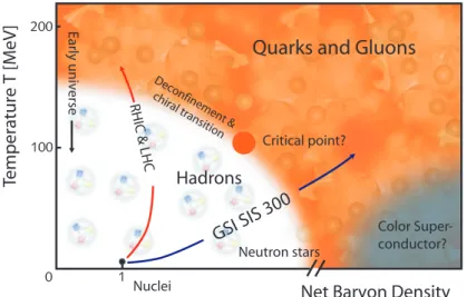
The visible matter in the universe consists of electrons and nucleons. While electrons are elementary particles, the nucleons are composites, made of quarks and gluons. According to our understanding of the evolution of the universe, nucle-ons emerged at a world age of about 10 µs out of a cooling soup of quarks and gluons, immersed in a plasma of leptons and photons. This picture rests on the physics of strong interaction and hadron structure. The basic theory of strong inter-action is Quantum Chromodynamics (QCD). Indeed, it predicts a transition from hadron matter, where coloured quarks and gluons are strongly correlated and con-fined in hadrons, to a quark-gluon plasma with much higher colour mobility of its constituents. In other words, in strongly interacting matter at not too large density and/or temperature hadrons are the relevant degrees of freedom. In contrast, at sufficiently large density and/or temperature quark and gluon degrees of freedom are important.
RHIC & LHC
GSI SIS 300
Net Baryon Density
Quarks and Gluons
Neutron stars Nuclei Temperatur e T [MeV] Early universe Hadrons Deconfinement & chiral transition Color Super-conductor? Critical point?
Figure 1.1: The phase diagram of strongly interacting matter in the physical case of 2 + 1 quark flavours. Shown is the rich structure of differ-ent phases (quark-gluon plasma and hadronic phase) and the importance in cosmology and astrophysical applications as well as the region of ther-modynamic space that experiments can investigate. For extremely dense matter a colour-superconducting phase of quark Cooper pairs is expected. Image from GSI [GSI1].
This idea has been considered by many physicists as so fascinating that they tried to investigate the transition to a novel state of strongly interacting matter under laboratory conditions. In fact, the collision of nuclei at high energies offers the possibility to transiently create the quark-gluon plasma and to experimentally investigate its properties by various probes. Apart from the idea to recover a stage of the cosmic evolution under laboratory conditions, insight into the behaviour of strongly interacting matter can be gained. This is indeed necessary for a more profound knowledge on cores of neutron stars, core dynamics in supernovae IIa
10 1 Introduction
and to put speculations about quark stars on firm ground. For all the phenomena mentioned, two issues are of ultimate importance - the phase diagram of strongly interacting matter and the corresponding equation of state.
A sketchy illustration of the phase diagram is exhibited in Figure 1.1, which may serve as a map for rough orientation. It is based on results of the basic theory of strong interaction, QCD, which is outlined in the next section. The phase diagram is discussed in some more details in section 1.2. In section 1.3, the no-tion “equano-tion of state” is introduced. It is pointed out that it is needed to describe the thermodynamics of matter and, at the same time, serves as input for dynamical calculations.
1.1
Quantum Chromodynamics
With the exception of gravitation, the fundamental interactions between the elemen-tary constituents of matter can successfully be described by means of gauge field theories. The quantization of gravity, either in the framework of string theories or by canonical quantization, did not yet reach a satisfying level. In analogy to Quantum Electrodynamics (QED), which is a very successful and very accurate gauge theory in physics describing electromagnetic interactions, strong interactions are formu-lated within the framework of QCD. But, whereas in QED the gauge bosons of the theory (photons), do not interact with each other, the non-Abelian SU(3) gauge group character of Yang-Mills type in QCD with its 8 associated coloured gauge bosons (gluons) and 6 quark species (spin 12 fermions) causes striking differences. Since gluons themselves carry the charge of the strong interaction (colour), they interact with each other, adding a variety of new processes.
The classical Lagrange density Ldescribing QCD is
LQCD= ¯ψ(iγµDµ−m)ψ− 1 4F µν a Fµνa +Lgauge+LFP, (1.1) where Faµν =∂µAνa−∂νAµa +gfabcAbµAcν, (1.2) Dµ=∂µ−igAaµTa, (1.3) [Ta, Tb] =ifabcTc. (1.4)
Apart from contributions from the fermionic sector (ψ) (flavour and colour indices being suppressed) and the gauge field sector (Aµa in Faµν)1 the gauge has to be fixed
in order to quantize the theory. This is accomplished by Lgauge. Furthermore, in
LFP possibly occuring unphysical degrees of freedom are taken care of by
intro-ducing Fadeev-Popov ghost fields. The kinetics of the quarks is expressed through the term involving the gauge covariant derivative Dµ, in which minimal coupling
between quarks and gluons is realized with coupling constant g. Ta are the
gene-rators of the local SU(Nc) gauge group2 in the fundamental representation, which
form an algebra. The multiplicative factors combining the generators of the Lie group with each other are the totally antisymmetric structure constantsfabc. Since
the field strength tensors Faµν contain, apart from terms well-known from Abelian
gauge theories such as QED, combinations of gauge fields, the pure Yang-Mills term
1The indicesµ, ν= 0, ...,3 refer to the Minkowski space-time and a= 1...8 is an adjoint colour
index counting the number of gluons.
1.2 The QCD phase diagram 11
consists of terms trilinear and quadrilinear in Aµa corresponding to self-couplings
among the gluons. The massesm of the current quarksψ (which are called quarks in the following) and the coupling strength g have to be adjusted to physical ob-servables.
QCD is a renormalizable theory and, thus, the couplingαs=g2/4π depends on
the considered momentum scaleQor is a function of the separation distance between the partons (quarks and gluons), correspondingly. In fact, neither quarks nor gluons have been directly observed in nature as isolated entities. Only hadrons (baryons and mesons), which consist of those partons combined to a colourless composite system, are measurable in the detector. As the separation distance between the partons increases, the energy scale drops resulting in an enormous increase in αs.
On the other hand, in the limit Q → ∞ the running coupling αs(Q) vanishes,
resulting in the fact that quarks and gluons can move quasi-freely. This is known as asymptotic freedom and has been experimentally verified in Deep Inelastic Scattering experiments. Thus, at sufficiently high energies, perturbation theory should be valid to evaluate processes of strong interaction within QCD, whereas perturbation theory breaks down as αs &1. In the latter regime, non-perturbative methods are needed
in order to solve the QCD equations3. One way in doing so is to discretize space and time and apply Monte Carlo sampling methods. This approach is called lattice QCD. In the following, this thesis significantly deals with such numerical results. For a short hand notation, the results will be named “lattice data”.
1.2
The QCD phase diagram
Asymptotic freedom tells us that at high momentum scales the running couplingαs
becomes small. Thus, in a hot and/or dense system, hadrons dissolve into a gas of quasi-free quarks and gluons. This new phase has been named quark-gluon plasma (QGP). The phase transition from the confined phase of strongly interacting matter to the QGP phase resulting in an increase of the relevant degrees of freedom has been dubbed (colour) deconfinement transition. Although the question about the nature of the phase transition - whether it is of first order, second order or even a crossover - decisively depends on the number of active quark flavoursNf as well as
their masses mq, the terminology “transition” is used in the following.
The Lagrangian in (1.1) is chirally symmetric for mq = 0. In the low energy
world that we live in and that we know from experience, quarks are massive (mu =md6= 0). But in systems that are sufficiently hot and/or dense chiral
symme-try gets restored, meaningmq→ 0 (chiral limit). Thus, there is another transition
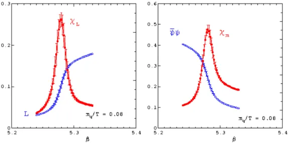
accompanied by the spontaneous breaking of chiral symmetry, which happens to be in the transition region of deconfinement. In Figure 1.2 the expectation values of the Polyakov loop hLi (cf. [Ris03]) and of the chiral condensate hψψ¯ i as the order pa-rameters of deconfinement and chiral symmetry restoration, respectively, as well as the according susceptibilities are shown as functions of the bare couplingβ = 6/g2.
The calculations were performed on the lattice forNf = 2 dynamical quark flavours.
To be more precise, in pure gauge theory (Nf = 0, mq → ∞) the expectation value
of the Polyakov loop is the order parameter of the deconfinement transition, where
hLi = 0 in the confined phase and non-zero in the deconfined phase. The order of the phase transition is dictated by the Z(3) centre symmetry. Since the lattice
3For an overview of non-perturbative methods the reader is referred to [Bla03a, Ris03] whereas
12 1 Introduction
calculations were performed using finite quark masses, Z(3) is explicitly broken re-sulting in a finite value of hLi in the confinement region. On the other hand, in
Figure 1.2: Order parameters (left: L - the Polyakov loop, right: ¯
ψψ - the chiral condensate) and corresponding susceptibilities χL,m of
deconfinement and chiral symmetry restoration. From [Kar02].
the chiral limit the order of the transition, depending on Nf, is controlled by the
chiral symmetry of the fermionic part in (1.1) with the expectation value of the chiral condensate as an order parameter. hψψ¯ i changes from a finite non-vanishing value in the phase where chiral symmetry is explicitly broken to zero in the chi-rally symmetric phase. Again, since the calculations use finite non-vanishing quark masses, hψψ¯ i does not vanish in the chirally symmetric region. The corresponding susceptibilities have a pronounced peak in the region of most rapid changes of the expectation values. This determines a critical bare couplingβc which translates into
a pseudo-critical temperature Tc. Astonishingly enough, βc seems to be the same
for both, deconfinement transition and chiral symmetry restoration, which indicates a strong correlation between them4.
If chiral symmetry would be exact in nature, its breaking would cause the existence of a massless hadronic Goldstone boson multiplett, but sincemu≈md>0
in nature, pions aquire a small mass. The finite value of the condensate
hψψ¯ i ∼ −(240 MeV)3 is caused by the fact that due to their interactions in hadrons the effective mass of confined quarks is much bigger than the mass of the almost massless (current) quarks.
The phase diagram of strongly interacting matter is shown in Figure 1.1. De-confinement and chiral symmetry transition separating the QGP and the hadronic phase happen at the transition temperature Tc and a pseudo-critical chemical
po-tential µc. Historically, µ denotes the chemical potential and µ = 0 refers to a
particle-antiparticle symmetric situation. Atµ= 0, lattice calculations foundTc to
be of the order of 170 MeV [Kar01] with a significant dependence on Nf and mq.
Accordingly, the heavier quark flavours (charm, bottom and top) are exponentially suppressed in the region of deconfinement5.
4For a possible explanation in a Polyakov loop model cf. [Pis00, Dum02].
5Only quarks with masses much smaller than the relevant temperature scale are considered to be
1.2 The QCD phase diagram 13
Applying universality arguments by examining the influence of global symme-tries, predictions can be made about the order of the transition. In the quenched limit with Nf = 0 and thus mu, md, ms → ∞ the transition is of first order
(cf. [Sve82, Yaf82]) and Tc is controlled by SU(3). This has been comfirmed by
calculations on the lattice [Boy96, Oka99]. In the chiral limit for Nf ≥ 3 with mu = md= ms = 0 the transition is of first order as well [Pis84]. However, in the
case of Nf = 2 (mu = md = 0, ms → ∞) it is an analytical crossover as it has
been shown on the lattice in [Got97, Scm02, Ali01a]. Thus, taking both results into account, there has to be a critical mass ms leading to a critical point where the
transition is of second order in the physical case ofNf = 2 + 1 active quark flavours.
This is the situation in whichmu =md ≈ 0 but ms is of the order of Tc. Lattice
calculations withms ∼Tc showed that the critical mass mcs≈ 12ms, indicating that
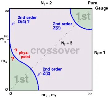
in the real world the deconfinement transition should be crossover. The dependence of the order of the transition on the number of active flavours and their masses is shown in Figure 1.3.
Figure 1.3: The quark mass and flavour dependence of the order of the hadronization transition at µ = 0. Thick lines indicate a second order phase transition, whereas the physical case of 2 + 1 quark flavours is believed to be crossover. From [Kar02].
The pseudo-critical temperature at µ = 0 has been calculated for two and three active quark flavours in [Kar01] and for the physical case of 2 + 1 flavours in [Fod02b]6 yielding T0 ≡ Tc(µ = 0) = (172±3) MeV and for the critical point TE = (160±3.5) MeV at baryon chemical potentialµE = (725±35) MeV. Thus, in
the physical case, the transition of deconfinement and chiral symmetry restauration is presumably of first order at large µwith a critical point of second order turning into a crossover forµ≈0.
Non-perturbative attempts to calculate the thermodynamics of strongly inter-acting matter are, for instance, phenomenological models or effective theories which are based on the symmetry of LQCD. There, the low energy behaviour of QCD 6The actual numbers decisively depend on the employed quark masses. Recent calculations
[Fod04], which have not yet been continuum extrapolated, find instead for physical quark masses T0= (164±2) MeV,TE= (162±2) MeV andµE = (360±40).
14 1 Introduction
is examined, e. g. in chiral perturbation theory based on the effective chiral La-grangian [Sce02]. A completely different approach for solving the theory are the above mentioned lattice QCD Monte-Carlo simulations in which strong interactions are quantized and evaluated in a discretized space-time (cf. Appendix D). In fact, pure gauge theory has been studied well, whereas including dynamical quarks is much more time consuming. In addition, for non-vanishing chemical potentialµthe quark determinant and thus the integration measure becomes complex. This results in complex Boltzmann weights which lead to oscillating signs7 making a standard Monte-Carlo calculation based on importance sampling impossible. Some of the details of such non-perturbative methods are reported in Appendices C and D.
In addition to the hadronic phase and the plasma phase of quarks and gluons, colour-superconducting and colour-flavour locked phases of quark matter are ex-pected in sufficiently dense systems (see [Pis99, Rus04] and references therein). One of these states is indicated in Figure 1.1. Furthermore, there is a nuclear liquid gas transition near the ground state of nuclear matter. None of those phases are an issue of this work, but should be mentioned for completeness. This thesis deals with the transition of deconfinement and chiral symmetry restoration.
1.3
The equation of state
Knowing the equation of state (EoS) is of significant importance. It describes the bulk properties of a medium in equilibrium. In a system contained in a box of volume
V, the properties temperature T, energyE, particle numberN, pressurep etc. can be attributed in a phenomenological approach. Among these quantities, there are certain relations, and other variables such as chemical potentialµ, free energyF etc. may be introduced in order to characterize the system under consideration. From thermodynamics it is known that the pressure of the system is a function of the temperature and the chemical potential. It is directly related to the grand canonical potential Ω through p(T, µ) =T·∂lnZ(T, V, µ) ∂V V→ ∞ −→ T·lnZ(T, µ) V =− Ω(T, µ) V , (1.5)
in the thermodynamic limit, where the volume of the homogeneous system under consideration becomes large, i. e. V→ ∞. Z is the partition function of the grand canonical ensemble. The other thermodynamic observables can be computed by knowing p(T, µ) using Euler’s and Gibbs’ relations
s(T, µ) = ∂p(T, µ) ∂T , n(T, µ) = ∂p(T, µ) ∂µ , ǫ(T, µ) =−p(T, µ) +T·s(T, µ) +µ·n(T, µ). (1.6)
s,nand ǫare the entropy, net number and energy densities, respectively. The EoS follows, for instance, as the dependence ǫ(p) with an additional independent state variable kept fixed. Thus, knowing the pressurep(T, µ) is sufficient for calculating the thermodynamics of strongly interacting matter.
The knowledge of the EoS is crucial for astrophysical observations, because cross-properties like the mass-radius relation of stars are governed by the Tolman-Oppenheimer-Volkov (TOV) equations, which need a relation ǫ(p) at T = 0 for
1.4 Outline of the work 15
finding solutions. Also Friedmann’s equations for the expanding universe need a similar relation as an input, say in the formp(ǫ, n). More generally, for determining the dynamics of a system within a hydrodynamical approach, the equation of state is needed, e. g., for integrating the Euler equations or, if dissipative effects are operative, the Navier-Stokes equations. In the latter case also transport coefficients like viscosities and heat conductivity are needed to characterize the system. How-ever, these quantities are not subject of the present work. The matter in neutron stars is cold and dense (T → 0, µ = 400−500 MeV) and one could imagine such classes of stars consisting of cold dense quark matter resulting in the possible existence of quark stars or quark cores in compact neutron stars.
In addition, from standard cosmology it is known that up to 10−5 s after the Big
Bang matter remained in the quark-gluon plasma phase. At a temperature of about 170 MeV8 confinement started and the hadronization of the QGP set in.
Furthermore, in heavy-ion collision experiments, in which ultrarelativistic nuclei collide at laboratory energies of about 1−100 GeV per nucleon, fireballs are created whose time evolution is governed to a large extent by the EoS. CERN SPS9gave the
first experimental indications of the existence of a phase in which quarks and gluons are quasi-free in a plasma. This has been confirmed at the Relativistic Heavy-Ion Collider (RHIC) at BNL, working on a higher energy regime than CERN SPS, up to
√s= 200 AGeV. In the future, the Large Hadron Collider (LHC) at CERN will start
to operate from 2007 and probe strongly interacting matter far above the critical temperature. In contrast, the envisaged Condensed Baryon Matter project of GSI in Darmstadt will investigate the phase boundary of the hadronization transition at not too high temperatures but at large baryon density [GSI2]. In relativistic heavy-ion collision experiments, the QGP is created intermediately and after thermalization (the typical time scale of the onset of QCD thermal matter formation is estimated by 0.5 fm/c) equilibrium thermodynamics governes the system. Thus, a description of the bulk of emerging particles by thermo-hydrodynamical models is possible.
1.4
Outline of the work
The subject of the present work is the equation of state of strongly interacting matter in the region near the “phase border line” depicted in Figure 1.1. The starting point is an analysis of results from lattice QCD within a phenomenological quasi-particle model (QPM). In chapter 2 this quasi-particle model is outlined. The description of how the model can be derived from QCD is relegated to Appendix E, since such a derivation is still subject of intense research. In chapters 3 and 4 sets of available lattice QCD data are analysed in detail. The quasi-particle model itself rests on work done by Peshier et al. [Pes96, Pes00, Pes02a]. However, in this thesis the new lattice data for µ >0 (cf. [All03, Kar03b, Fod03a]) are quantitatively analysed. Basing on the parameters found in the analysis, the quasi-particle model is used to extrapolate the equation of state in the region of large baryon density. The quantitative results are summarized in chapter 5. This region is not yet accessible by lattice QCD or other methods based on first principles. In chapter 5, consequences of the results are also discussed, such as implications on quark stars or on central heavy-ion collision
8We use particle physics units with ~c = c = kB = 1 in which energy, momentum and
temperature are given in GeV or MeV. To convert the temperature, from the definition of kB, 1K= 8.617·10−5 eV follows.
9The Super Proton Synchrotron (SPS) works at beam energies up to 158 AGeV for lead projectiles
16 1 Introduction
experiments. Partial results of the research described in this thesis are reported in [Blu04, K¨am04].
2
Quasi-particle model
In this chapter, the quasi-particle model is introduced which is used in this thesis. Considering the thermodynamics at momenta k ∼ T and k ∼ µ, only transverse gluonic and quark single-particle excitations give contributions. These excitations propagate predominantly on mass shell in the plasma phase. Basing on temperature and chemical potential dependent self-energies Π due to medium effects, the arising quasi-particle excitations obey dispersion relations near the light cone which can be approximated byω =√k2+ Π +m2 (cf. [LeB96, Pes98b]). The model was first
introduced for describing the pureSU(3) gluon plasma in [Pes96]. Employing per-turbative thermal masses from an improved HTL scheme, the quasi-particle model was also tested forSU(3) in [Lev98]. Later, it was extended to the case ofNf = 2,4
dynamical quark flavours and non-vanishing chemical potential in [Pes00, Pes02a]. The development of this model was inspired by work in [Bir90, Ris92, Pes94].
2.1
Description of the model
In the region of small coupling g2, the soft momenta k ∼ gT are much smaller
than the hard momenta k∼T. Comparing both contributions in the loop-integral expressions of, e. g., the self-energies Πiof the QCD excitations1, the hard excitations
dominate [Kap89, LeB96]. Therefore, the transverse gluonic and positive fermionic branches propagate predominantly on mass-shell, whereas the longitudinal plasmon as well as plasmino excitations2 are exponentially suppressed. Furthermore, the QGP has to be considered as a physical system with medium dependent dispersion relations, because in the plasma phase the interacting quarks and gluons are in a hot bath of themselves. Such in-medium effects can be taken into account by considering single-particle excitations as massive quasi-particles3. The model’s simplicity rests on the neglect both of a possible imaginary part of Π and of any possible momentum and energy dependences of Π. Due to these significant approximations, the model must be carefully checked against lattice QCD results. Anticipating the success of the model, the advantage is that the term Π +m2 can formally be considered
as an effective state dependent mass, m(T, µ). It needs to be proven that all the complexity of QCD interactions can be condensed into such a simple form, at least for the EoS.
As has been shown in [Gor95], fundamental thermodynamic relations such as Gibbs’ relation and thermodynamic self-consistency are maintained, when consider-ing a system withω =ω(k, m(T, µ)). Additional medium contributions have to be included which can be done by introducing an effective HamiltonianHeff =Hid+E0∗.
E∗
0(m(T, µ)) is an additional finite “potential energy”, which represents the system’s 1The labelirefers to the various quark flavours and the gluon.
2They are called collective excitations.
3In fact, the description of in-medium properties by adopting a system of massive quasi-particles
has been very successful in various fields of physical interest, e. g. in Solid State Physics. For our case, the poles of the propagators have been analysed for T = 1.5T0 and 3T0 [Pet02] where
18 2 Quasi-particle model
energy in the absence of quasi-particle excitations. It cannot be subtracted, since the system’s lowest energy state becomes T and µ dependent. The pressure p and energy densityǫfollow from statistical mechanics, where, in addition to the standard expressions (cf. [Lan66]), a term proportional toE∗
0 arises.
The quasi-particle model rests on the description of the quark-gluon plasma as a gas of weakly interacting massive quasi-particles with residual interactionB, where the medium contributions are taken into account through
B = lim
V→∞ E∗
0
V
in the thermodynamic limit. Considering a gas of light quarks (u- and d-quarks commonly are denoted as q), strange quarks (s), and gluons (g), the pressure can be written in compact form as
p(T, µ) = X
i=q,s,g
pi(T, µi;m2i(T, µ))−B(m2j(T, µ)). (2.1)
The pi refer to the contributions of the different partons with medium dependent
respective dispersion relations
pi(T, µi;m2i(T, µ)) = di 6π2 Z ∞ 0 dkk 4 ωi [f+(ωi) +f−(ωi)]. (2.2)
Formally, equation (2.2) looks like the ideal gas pressure, however, with the sub-stantial modification m(T, µ) instead of a rest mass m. The distribution functions
f+ and f− are given through
f±(ωi) =
1 e(ωi∓µi)/T +S
i ,
where the dispersion relation for the hard excitations near the light cone is given by
ωi =
q
k2+m2
i(T, µ). Having written down the pressure in the form (2.2) the
contributions stemming from the corresponding antiquarks have already been taken into account through the terms proportional to f−(ωq) andf−(ωs). Hence, they do
not need to be summed up in (2.1). The chemical potential is µq=µ for the light
quarks andµg = 0 for the gluons4. In the case of vanishing quark chemical potential µq = 0, a matter-antimatter symmetric system is under investigation. Therefore,
restricting the attention on vanishing net strangeness,µs = 0 has to be set. The spin
factors are given bySq =Ss= 1 andSg=−1, taking care of the different statistics5.
As for free partons, the degeneracy factorsdi, taking the two spin degrees of freedom
for quarks into account, are dq = 2NqNc, ds = 2Nc and dg = Nc2−1. Nq is the
number of light quark flavours and the factor of 2 gluon polarizations has been absorbed in (2.2), since
n(ωg) =
1
2[f+(ωg) +f−(ωg)].
4Gluons, being the gauge bosons of the strong interaction, must have vanishing chemical potential
in thermodynamic equilibrium, since their particle number is not a conserved quantity.
5Quarks, being fermions, obey the Fermi-Dirac statistics, whereas gluons, being bosons, obey
2.1 Description of the model 19
The expressions for the entropy densitysand the number densitynin the quasi-particle model are then obtained by using Euler’s relations (1.6)
∂p ∂T µ =X i ∂pi ∂T µ − ∂B∂T µ =X i ∂pi ∂T µ;m2 i +X i ∂pi ∂m2i ∂m2 i ∂T µ − ∂B∂T µ (2.3) and ∂p ∂µ T =X i ∂pi ∂µ T − ∂B ∂µ T =X i ∂pi ∂µ T;m2 i +X i ∂pi ∂m2 i ∂m2 i ∂µ T − ∂B ∂µ T . (2.4)
The pressure p is a function of T and µ, both explicitly and implicitly through
m2j(T, µ). From the stationarity property of the thermodynamic potential under functional variation of the effective massesm2j [Gor95]
∂p ∂m2 j T,µ,m2 i6=j = 0 (2.5)
follows. Ensuring thermodynamic self-consistency, a condition on the residual inter-action follows immediately
∂B ∂m2 j = ∂pj ∂m2 j . (2.6) Consequently, ∂B(m2 i(T, µ)) ∂T µ = X i ∂B ∂m2 i ∂m2 i ∂T µ =X i ∂pi ∂m2 i ∂m2 i ∂T µ , (2.7) ∂B(m2 i(T, µ)) ∂µ T = X i ∂B ∂m2i ∂m2 i ∂µ T =X i ∂pi ∂m2i ∂m2 i ∂µ T (2.8) can be found. Thus, comparing with (2.3) and (2.4), the entropy density s and number density n are given by the standard expressions with vanishing residual interactions s = X i ∂pi ∂T µ;m2 i =X i si, (2.9) n = X i ∂pi ∂µ T;m2 i =X i ni =nq (2.10)
in the case of non-strange matter. In fact,sand nbeing combinatorical expressions of p and ǫ through Gibbs’ relation cannot depend on the system’s lowest energy state. The explicit expressions forsi and ni are given by
si = di 2π2T Z ∞ 0 dkk2 ( 4 3k2+m2i q k2+m2 i [f+(ωi) +f−(ωi)] −µi[f+(ωi)−f−(ωi)] ) , (2.11)
20 2 Quasi-particle model nq= dq 2π2 Z ∞ 0 dkk2[f+(ωq)−f−(ωq)]. (2.12)
The energy density follows from (1.6) and reads
ǫ=B(T, µ) + X i=q,s,g di 2π2 Z ∞ 0 dkk 4 3T ( e(ωi−µi)/Tf2 +(ωi) +e(ωi+µi)/Tf2 −(ωi)− T ωi [f+(ωi) +f−(ωi)] ) . (2.13)
It should be emphasized that equations (2.11, 2.12) formally look like the corres-ponding expressions for the ideal gas, again with m(T, µ).
Now, the quantities mi need to be specified. The effective medium dependent
masses mi of the partons are given through (cf. (2.1))
m2i =m2i;0+ Πi(k;T, µ), (2.14)
where m2i;0 are rest mass contributions. To take perturbative aspects of QCD into account, the Πi(k;T, µ) are taken to be the one-loop self-energies at hard momentum k. They are given through [Kap89, Pis89, Pes98b]
Πg = Nc+ Nq+Nh 2 T2+ 3 2π2 X i=q µ2i g2 6 , (2.15) Πq,s = 2mq,s;0ωq,s+ 2ω2q,s, (2.16) ω2q,s = N 2 c −1 16Nc T2+ µ 2 q,s π2 ! g2, (2.17)
where Nh = 1 in the presence of strange quarks and zero elsewhere. If mq;0 of the
current quarks is of the order of gT, the addition of the self-energies and the rest mass contributions would be somewhat more involved. This becomes clear when looking at the renormalized fermion propagators [Pis89]. The effect is important when considering strange quarks or temperature dependent “rest” masses which are introduced in lattice QCD calculations due to computational limitations. Details are discussed in chapter 3. Nevertheless, in the chiral limit as well as for light quark flavours m2
q reduces tom2q = Πq = 2ωq2.
Given the severe approximations made, sufficient flexibility must be introduced to go beyond, say, one-loop self-energies. The decisive step lies in replacing the run-ning couplingg2 from perturbative QCD by an effective couplingG2(T, µ), following
the renormalization group equation. In two-loop order the QCD result is [Hag02]
g2(¯µ) = 16π 2 β0ln(¯µ2/Λ2) 1−2β1 β2 0 ln ln(¯µ2/Λ2) ln(¯µ2/Λ2) ! , β0 = 11− 2 3Nf, β1 = 51− 19 3 Nf, (2.18)
neglecting the term involving ln−2(¯µ2/Λ2) which gives only a small correction for ¯
µ ≈ Λ2. ¯µ is the renormalization scale6 and Λ is the scale parameter of QCD 6It is usually chosen to be proportional to the first Matsubara frequency, i. e. ¯µ= 2πT.
2.2 Extension to finite chemical potential 21
which is fixed by the comparison of theoretical results with experimental data. In thermodynamic equilibrium the mean value of all momenta is ¯k ∼ T. Thus, ¯µ
and Λ are proportional to T, or, more precisely, Λ → Tc/λ, Tc being the relevant
temperature scale of the deconfinement transition7. In order to phenomenologically regularize the divergent effective running coupling asT →Tc, a shift parameter Ts
is introduced8 G2(T, µ= 0) = 16π 2 β0ln T−Ts T0/λ 2 1−2β1 β2 0 ln lnT−Ts T0/λ 2 lnT−Ts T0/λ 2 . (2.19)
Note, again, that T0 denotesTc(µ = 0). Non-perturbative effects in the vicinity of
the transition temperature (compare Appendix C) are modeled by replacing g2 in equations (2.15, 2.17) with G2. For T ≫ Ts the effective coupling approaches the
perturbative result g2. Having introduced two parameters λ and T
s, both have to
be adjusted to the lattice results.
Expanding (2.1) into a series ing2, the perturbative results up to next-to-leading order (NLO) p0 +p2 (compare Appendix C) are completely reproduced including
some parts of higher order corrections. To be more precise, only 1/√32 of the
g3-term, which is called the plasmon term, is included in the model. But it is exactly theg3-term which spoils the convergence of the perturbative series. However, in its
unexpanded form, (2.1) is a thermodynamicly consistent resummation of all orders ing2, making the model valid even in the strong coupling regime in the vicinity of the phase border line.
In massless Φ4-theory the outlined structure of the entropy density emerges by
resumming the super-daisy diagrams in tadpole topology [Pes98a]. It can be argued that such an ansatz is valid for QCD as well [Pes01]. In section 2.3 and Appendix E the model is put on firmer ground by listing the chain of approximations necessary for arriving at the QPM described above when starting from QCD.
Furthermore, the residual interaction B has to be computed. This can be achieved by performing an appropriate line integral in the µ-T plane, which is ex-plained in detail in the following section. From (2.7) and (2.8)
B(T, µ) =B0+ Z ∂B ∂T µ dT + ∂B ∂µ T dµ ! =B0+ X i Z ∂pi ∂m2i ∂m2i ∂T dT + ∂m2i ∂µ dµ (2.20)
is found, where the integration constant B0 has to be adjusted to lattice data as
well. The corresponding derivatives are calculable in a straightforward manner. The equations (2.1) and (2.2), (2.11) - (2.13) together with (2.14) - (2.17) and, optionally, (2.19) define the model.
2.2
Extension to finite chemical potential
Eventually, the effective coupling G2 has to be known for all T and µ in order to calculate the thermodynamic quantities. Thus, when knowing G2 at µ = 0 from
7From lattice calculations forNf = 2,Tc= 0.49Λ(2) ¯
M S has been advocated in [Gup01].
8In fact, it is this modified effective coupling allowing to appropriately describe the lattice data
22 2 Quasi-particle model
fitting lattice data, G2 can be mapped into the µ-T plane by imposing Maxwell’s relation onto p. The pressure is a potential of the state variables T and µ [Pes00], i. e. ∂2p ∂µ∂T = ∂2p ∂T ∂µ (2.21) forµ6= 0. Therefore ∂s ∂µ − ∂n ∂T = 0 (2.22) holds, resulting in X i=q,s,g ∂si ∂m2 i ∂m2i ∂µ − ∂nq ∂m2 q ∂m2q ∂T = 0. (2.23)
The thermodynamic entities depend on T and µ both explicitly and implicitly through mi, where the explicit derivatives vanish upon imposing Maxwell’s relation
on pq using (2.9) and (2.10). In the derivatives with respect to m2i,mi depends on
the state variables both explicitly and on the effective coupling G2(T, µ). In this
way, a partial differential equation (PDE) for G2(T, µ) can be derived, which is of first order and linear in the derivatives of the coupling but non-linear in theG2 itself. We call this the flow equation,
aT ∂G2
∂T +aµ ∂G2
∂µ =b, (2.24)
which can be solved given a valid boundary condition. Thus, knowing the effective coupling at, for instance, G2(T, µ = 0) as in (2.19) or G2(T = 0, µ) is sufficient for solving the PDE. It should be emphasized that for any given set of G2 on a curve
µ(T) or T(µ), G2 can be determined in a certain region of µ-T. The PDE can be
solved by the method of characteristics [Pes02a]. Introducing a curve parameter x,
aµdT(x) = aTdµ(x), (2.25)
aµdG2(x) = bdµ(x) (2.26)
are yielded as characteristic equations from (2.24).
The explicit form of the coefficients aT, aµ and b, which depend on T, µ and G2, as well as their algebraic derivation can be found in Appendix A. They obey
aT(T, µ → 0) = 0, aµ(T → 0, µ) = 0, aµ(T, µ → 0) 6= 0 and b(T, µ → 0) = 0.
As a result, the characteristic curves T(µ(x)) end perpendicular into the T and µ
axes. Furthermore, whenG2 →0, the coefficientbvanishes resulting indG2/dµ= 0 from (2.26). Thus, G2 is constant along the characteristic curves in the asymptotic region. The curves become ellipses [Pes00], which are given through
4Nc+ 5Nf 9Nf T4+ 2T2µ 2 π2 + µ4 π4 = const. (2.27)
This is still approximately true for G2 6= 0, but as the effective coupling increases
at µ = 0 the elliptic pattern changes and the curves become flatter (compare sec-tion 4.2.2).
Following the outlined path, the lattice QCD data given atµ= 0 can be mapped to finite values of the quark chemical potential and small temperatures9. As long
9In contrast, calculations on the lattice seem to be limited to small µ [Fod03a]. As argued
2.3 Foundation of the model 23
as the model is valid, the thermodynamics of the quark-gluon plasma can be cal-culated for a certain region in (µ, T). It should be noted that the parametrization (2.19) for µ = 0 makes contact with perturbative QCD. Near T0 or even below T0
another parametrization may be more appropriate. Given an integration constant
B0, the residual interaction B(T, µ) can be computed through integrating along a
characteristic curve. SinceT and µare both functions ofx,B and m2
i depend on x
as well. Hence, from (2.6)
dB(x) dx = X i ∂B ∂m2i dm2i dx = X i ∂pi ∂m2i ∂m2i ∂T dT dx + ∂m2i ∂µ dµ dx + ∂m2i ∂G2 dG2 dx (2.28) follows, where the derivatives ofT,µand G2 with respect tox are known from the flow equation (2.24). GivenB atx′ = 0, meaning (µ′, T′) = (0, T∗), (2.28) has to be integrated over x′ up tox′ = x, meaning (µ′, T′) = (µ, T). Finally, the integration constantB0=B(T∗, µ= 0) can be determined by integrating (2.7) over T at µ= 0
fromT0 towards T∗. The remaining integration constant B(T0, µ= 0) of the latter
integration has to be fixed by lattice data.
2.3
Foundation of the model
The model outlined above has intuitively been introduced in [Pes94]. As already mentioned, some support comes from super-daisy resummed massless Φ4 -theory [Pes98a]. As argued in [Van98, Pes01, Bla01, Pes02b], the structure applies also in gauge theories with a fermionic sector even when including a finite width of the quasi-particle excitations [Pes04]. In Appendix E a sequence of approximations is described which is necessary for “deriving” the model from full QCD within a Φ-derivable approximation scheme. It should be noted that this “derivation” is not a rigorous one. More ambitious approaches [Bay62, Bla99b, Van00, Bla01] found a more involved structure than the one described in section 2.1. But, as shown in chapters 3 and 4, lattice data can be described by employing an effective coupling
G2 in the form (2.19). Therefore, the model used here should be termed simple phenomenological quasi-particle model.
Considering the thermodynamics of massless Φ4-theory as a starting point in a systematic approach, the bare Lagrangian reads
L= 1 2(∂µφ)(∂ µφ) −g 2 0 4!φ 4. (2.29)
Employing the Luttinger-Ward theorem onto the grand canonical potential Ω [Lut60], Ω is related to the exact propagators and exact self-energies of the theory. Its sta-tionarity property
δΩ
δ∆ = 0, (2.30)
ensures thermodynamic consistency in analogy to (2.5). In [Pes98a], the self-energies are considered in tadpole approximation which implies the restriction onto the first term in the skeleton contribution to Ω. In tadpole approximation, the self-energies Π(1) are momentum independent and real resulting in the fact that
the corresponding propagators ∆(1) contain the free propagators and a term which formally looks like a mass. By identifying Π(1) with m2, the dependence of m on the temperature becomes obvious. In fact, this procedure is scale independent and self-consistent since the occuring divergencies and the terms depending on the scale cancel.
24 2 Quasi-particle model
Given the pressurep=−Ω(1)/V, the entropy densitys=∂p/∂T is given through
an expression which formally looks like the standard thermodynamic expression. Furthermore, the entries in the dispersion relation look formally like temperature dependent thermal masses.
In QCD, the self-energies are momentum dependent and complex even at 1-loop order. However, when neglecting Landau damping terms and the momentum de-pendence of Π as in section 2.1, the entropy densitysis again given by the standard expression of massive quasi-particles, cf. Appendix E.
For cold QCD matter at finite density, an analogous quasi-particle model with a mass depending on µ is described in [Bai00], whose results are compared with hard thermal loop (HTL) perturbation theory at leading order. There, the model’s pressure was found to be equal to the weak coupling expansion through O(α2
s),
indicating that the quasi-particle approximation of a quark-gluon plasma at T = 0 is a very good effective description.
2.4
Comparison with other approaches
Due to the still lacking rigorous foundation of a model which describes the lattice QCD data down to Tc, various different phenomenological approaches have
been proposed in the literature. Here, a few of them are mentioned.
The quark-gluon plasma liquid model [Let03] is based on the lowest order ther-mal perturbative contribution to the pressure with temperature dependent non-perturbative coupling g2 ∼ α
s and includes a bag constant B. In other words, the
quark-gluon plasma is described by perturbative quark and gluon degrees of freedom. The temperature dependence of αs(T) is inferred from the running coupling αs(x) by setting an energy scalex and integrating the renormalization group
equa-tion with the β-function in 2-loop approximation. Furthermore, reasonable thresholds for the heavier flavours are included. As an effect of the occuring finite quark masses, corrections to the partition function but also thermal gluon masses are included in this ansatz [Let03]. However, near the pseudo-critical temperature
Tc(µ= 0), a disagreement between the model results and the lattice data [Fod03a]
has been observed. This is due to the fact that non-perturbative aspects of QCD are not taken into account in the model. Nevertheless, in [Let03] the thermodynamic quantities have been described fairly well at and above T ≥1.1T0 with decreasing
accuracy for increasing quark chemical potential. Moreover, by simply setting the quark masses zero as a chiral limit, the finite quark mass effects have been found to be negligible.
The quasi-particle model with appropriate thermal masses of the quasi-particle excitations was modified by the phenomenological parametrization of the confine-ment transition in the vicinity of T0 in [Sch01]. This was motivated by the fact
that the picture of a non-interacting gas near T0 is not valid. In fact, it was
ar-gued that the observed decrease of the thermodynamic quantities approaching T0
from above is caused by the change of the number of thermally active degrees of freedom, rather than a change in the masses, cf. section 2.1 and section 3.2. Thus, an effective, temperature dependent number of degrees of freedom di(T) =C(T)di
was introduced. C(T) is the confinement factor which is thought to be the same for quarks and for gluons. In contrast to the model described in section 2.1, the masses of the quasi-particles do not increase but follow roughly the behaviour of the Debye screening mass asT0 is approached from above. As a consequence a dropping
2.4 Comparison with other approaches 25
approximated by a critical power law behaviour. However, since the Debye screening mass is related to the longitudinal part of the self-energies, but the thermal masses are related to the transverse parts of Π, a direct comparison between the two models is more subtle.
In [Tha03] the model was extended to finite quark chemical potential imposing Maxwell’s relation in analogy to the procedure described in section 2.2. Thereby, a set of first order quasilinear partial differential equations for the effective coupling
G2(T, µ) and the confinement factor C(T, µ) was derived.
In [Rom02] a natural extension of the QPM was proposed. There, only weakly interacting quasi-particle excitations, which are determined by their HTL propaga-tors, were considered with vanishing residual interaction. The model is based on the HTL resummed entropy (cf. Appendix E), where the momentum dependence of the HTL self-energies and propagators of the quasi-particles as well as Landau damping effects are taken into account. However, in Φ-derivable approximations at 2-loop level the same picture emerges, and thus, the entropy of the hard thermal loop quasi-particle model (HTLQPM) was defined as in the Φ-derivable approxima-tions. Therefore, the model also serves as a good approximation to the full QCD result of the entropy, cf. [Bla01]. The expression for the pressurep follows directly from the stationarity property of the grand canonical potential Ω. Expanding the HTLQPM expression of p into a perturbative series in powers of g2 at vanishing chemical potential, the first terms of the series are reproduced, cf. Appendix C. Furthermore, 25% of theg3-term are included in the model, which is approximately
a factor 1.4 more than in the simple QPM.
In order to incorporate even more of the perturbative plasmon term, which is responsible for the bad convergence observed in the weak coupling expansion, the full momentum dependent next-to-leading order corrections to the self-energies need to be included. However, this is indeed hard to calculate and thus this contribution was approximated by the averaged contribution to the asymptotic masses in a next-to-leading order extension of the HTLQPM in [Reb03]. By introducing a cut-off scale which separates the soft from the hard momenta, a new parametercΛwas introduced
into the model. Estimating the influence of an inclusion of the full plasmon term by varyingcΛ, it was found that the stability of both quasi-particle models, QPM and
3
Comparison with lattice -QCD data
at
µ
= 0
In this chapter, results of lattice calculations atµ= 0 are quantitatively analysed. Over the years, the lattice evaluation codes have been improved. Improved actions, which minimize discretization errors, have been employed and more systematics has been accumulated. This requires to extend previous tests of the QPM to current lattice data. In section 3.1 such previous tests are recalled. One major result of this thesis is the detailed comparison of the latest lattice data for Nf = 2 + 1 with the
QPM, which is presented in section 3.2. The new feature is the extension of the model to describe the lattice data belowT0. From previous work it seems clear that
aboveT0 the model is successful. But, focussing here on describing the data in the
vicinity of the confinement transition, the results can be compared with results from a hadron resonance gas model forT < T0 [Kar03a]. Since the quasi-particle model
turns out to cover appropriately the data in the confinement region, the possible indication for quark-hadron duality is discussed.
3.1
Previous comparisons of the QPM with lattice - QCD
data
It has been proven that the QPM successfully describes the lattice data for temperatures above and equal T0 for the pure gluon plasma [Pes94, Pes96] and for
the quark-gluon plasma with various numbers of quark flavours [Pes00]. Since, due to computational reasons, the lattice calculations still employ heavy quark masses, it is worth to stress that the continuum-extrapolated and renormalization-group-improved lattice data for pure SU(3) gauge field theory is perfectly described by the QPM [Pes96, Pes00]. These data can be considered as final results. In contrast, the lattice data for various quark flavours are not yet systematically continuum-extrapolated. Moreover, the quark masses are frozen to unphysically large values, which not yet allow for a sensible chiral extrapolation. Nevertheless, the previous lattice data can successfully be described by the QPM, as demonstrated in [Pes00, Pes02a]. There, the data forNf = 2 and Nf = 4 have been considered in detail.
3.2
Test of the model for
N
f= 2 + 1
First, the lattice data for Nf = 2 + 1 based on [Kar00] are considered in detail.
An improved representation of these data can be found in [Kar03a], where also the region below T0 is resolved. T0 = 170 MeV is used in the following. The
data [Kar00, Kar03a] are obtained for a tree-level improved p4-action of staggered fermions on a 163 ×4 lattice. The entropy density s given in (2.9) and (2.11) allows for a straightforward mapping of the lattice data fors(T) onto the effective coupling G2(T, µ = 0). In this way, the parameters of the coupling in (2.19) can easily be fixed. In contrast, by fitting the lattice data of the pressure, an additional
28 3 Comparison with lattice -QCD data at µ= 0
integration constant B(T0) is needed. Following the lattice calculations in [Kar00],
the rest mass contributions are given by the temperature dependent lattice masses
mi;0 =aiT with aq =a= 0.4, as = 1.0 and ag = 0. Using (2.19) for T ≥T0, the
entropy density can be described by parametrizing the effective couplingG2 through a linear function in T for T < T0. Thus, going down inT from the deconfinement
region into the region of confinement the logarithmically divergent effective running coupling changes into a coupling moderately linear rising at T0
G2(T) = eq.(2.19), T ≥T0 G2(T 0) 1−αT0T (1−α) , T < T0. (3.1)
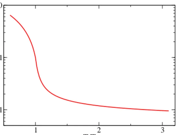
The effective coupling G2(T) normalized to its value at T0 is exhibited in
Figure 3.1. The optimal parameters to describe the entropy density (see below) areTs= 0.8T0,λ= 7.6 andα= 0.93. 1 2 3 T/T 0.1 1 10 G²(T)/G²(T ) 0 0
Figure 3.1: The effective coupling G2(T) normalized to G2(T 0) as a
function of the temperature in units of the pseudo-critical temperatureT0
forNf= 2 + 1.
The corresponding entropy density sis shown in Figure 3.2 and compared with the lattice data gained by using both, [Kar00] and [Kar03a], as references. An impressively good description of the data can be observed. Even more fascinating is the fact, that the lattice results can successfully be described below T0 with
this parametrization. In fact, no other order parameter changing at T0 is needed
to explain the behaviour below and above the phase transition temperature. All subtleties of the transition are encoded in the used parametrization of G2(T). This is possibly related to the fact that the entropy density is a measure for the density of states.
Having fixed the parameters inG2(T), the pressurepand the energy densityǫcan
be computed by determining an additional integration constant. According to (2.1) and (2.20), B(T0) usually is fixed by requirering p(T0,0)lattice = p(T0,0)QPM. The
results for p and ǫ usingB(T0) = 0.5T04 compared with the lattice data are shown
in Figures 3.3 and 3.4, respectively.
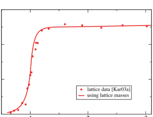
inte-3.2 Test of the model forNf = 2 + 1 29 1 2 3 T/T 0 5 10 15 20 s(T)/T³ 0
lattice data [Kar00,Kar03a] using lattice masses
χ-extrapolation
Figure 3.2: The entropy density s scaled byT3 forN
f = 2 + 1 as a
function of T /T0. The full line corresponds to calculations considering
the lattice masses as rest masses, the dashed line is the corresponding calculation using mi;0 = 0 as an estimate of the chiral extrapolation.
Lattice data from [Kar00, Kar03a].
grating B(T)−B(T0) = Z T T0 dB(T′) dT′ dT ′ =−X i di 2π2 Z T T0 dm2 i(T′) dT′ Z ∞ 0 dkk2 q k2+m2 i(T′) 1 (e√k2+mi2(T′)/T′ ±1) dT′. (3.2)
Obviously, the total derivative of B(T) with respect to T is directly proportional to the total derivatives of the massesm2
i(T) with respect to T. The result ofB(T)
is shown in Figure 3.5. After forming a maximum in the vicinity of the transition regionB(T) becomes negative for a certain value ofT /T0and approaches a constant
30 3 Comparison with lattice -QCD data at µ= 0 1 2 3 T/T 0 1 2 3 4 p(T)/T 4 0
lattice data [Kar03a] using lattice masses
χ-extrapolation
Figure 3.3: The pressure p scaled by T4 for N
f = 2 + 1 as a
function of T /T0. The full line corresponds to calculations considering
the lattice masses as rest masses, the dashed line is the corresponding calculation using mi;0 = 0 as an estimate of the chiral extrapolation.
Lattice data from [Kar03a] which correspond to the continuum extrapolated data from [Kar00].
1 2 3 T/T 0 5 10 15 ε (T)/T
lattice data [Kar03a] using lattice masses
4
0
Figure 3.4: The energy density ǫ scaled by T4 for N
f = 2 + 1 as a
function ofT /T0. The calculation uses the lattice masses as rest masses.
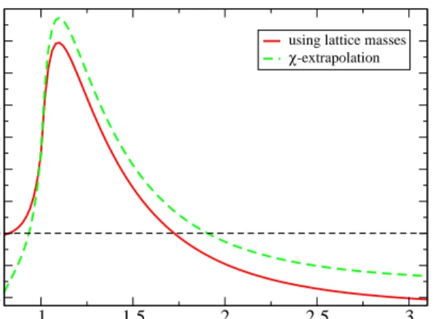
3.2 Test of the model forNf = 2 + 1 31 1 1.5 2 2.5 3 T/T -0.4 -0.2 0 0.2 0.4 0.6 0.8 1 1.2 B(T)/T 4 0
using lattice masses
χ-extrapolation
Figure 3.5: The residual interactionB(T) scaled byT4 forN
f = 2 + 1
as a function ofT /T0. The full line corresponds to calculations considering
the lattice masses as rest masses, the long-dashed line is the corresponding calculation usingmi;0= 0 as an estimate of the chiral extrapolation. The
horizontal short-dashed line marks the zero to highlight the change of sign inB(T) at about 1.72T0.
In Figures 3.2, 3.3 and 3.5, the extrapolations to the chiral limit settingmi;0= 0
in the calculations are represented by the dashed curves. The parameters inG2(T)
as well asB(T0) are kept fixed. As expected, when considering the thermodynamic
integrals in the pressure expression (2.2),p should increase for decreasing tempera-ture. This is due to the fact that the quasi-particle excitations become lighter when setting the rest masses to zero. Correspondingly, the residual interaction in (3.2) should decrease due to its proportionality to the derivatives of the masses with re-spect to the temperature. More precisely, the additional terms in the derivatives stemming from the temperature dependent rest masses (compare (A.10)), which compensate for the contribution coming from the derivative of the coupling, van-ish when setting the rest masses to zero. However, this extrapolation to the chiral limit is far too simple. In fact, lattice results for variousmi;0 are needed for a more
profound extrapolation in order to estimate the dependence of the parameters in
G2(T) andB(T
0) onmi;0. Furthermore, the extrapolation to the physical case also
depends onT0, which has to be taken into consideration.
As evident from Figures 3.2, 3.3 and 3.4, lattice data can impressively good be described even below T0 employing only quark-gluon degrees of freedom. In
con-trast to the quasi-particle model, the hadron resonance gas model used in [Kar03a] describes the data equally well below and at T0. But, in the resonance gas model
many heavy resonances up to 2 GeV are needed. In fact, atT0 the lightest hadron
contributions to the energy density are of the order of 15%. Furthermore, the hadron masses have been changed in order to mimic the heavy u and d quark masses em-ployed in the lattice calculations. In some sense, the quasi-particle model results correspond to this observation, since fairly heavy quasi-particle excitations emerge belowT0 due to the enormous increase inG2(T). The quasi-particle masses mi(T)
32 3 Comparison with lattice -QCD data at µ= 0
are shown in Figure 3.61. Thus, the large number of excited hadron states2 atT < T0
can effectively be described by a small number of quasi-particle excitations.
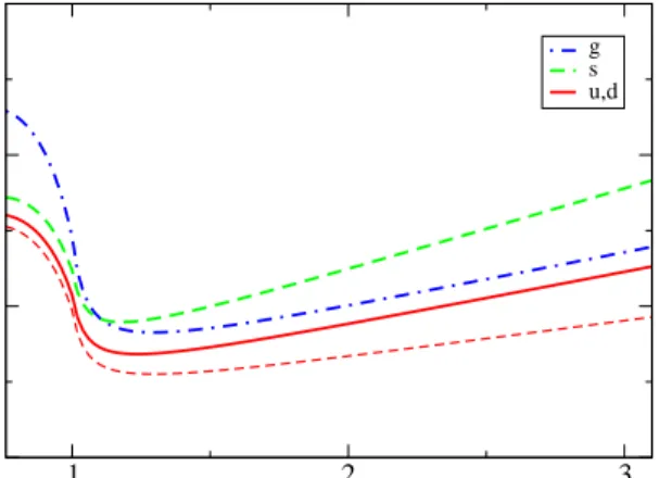
1 2 3 T/T 0 0.5 1 1.5 m (T)/GeVi 0 g s u,d
Figure 3.6: The quasi-particle massesmi(T) in GeV as a function of
T /T0. The full line, long-dashed line and dash-dotted line correspond to
light quark, strange quark and gluon masses, respectively. At and below the transition temperature, the masses of the quasi-particle excitations increase rapidly causing the sharp decline ofs/T3, p/T4 and ǫ/T4. The
thinner short-dashed line indicates the result for the light quarks when settingmq;0= 0 as an estimate of the chiral extrapolation.
Encouraged by the success of the QPM in describing lattice data also below T0
in the confined phase of hadrons, it could be speculated, whether there is a quark-hadron duality at work in a restricted interval around T0. In this case, hadron
observables could be expressed in a quark-gluon basis and vice versa. For instance, the hadron resonance gas model in [Kar03a] agrees with the lattice data in a narrow region above T0. Even more striking, a modified resonance gas model introducing
a finite, medium dependent width of the resonances describes the lattice data of the energy density above T0 very well [Bls03]. Allowing the resonances’ widths to
grow exponentially with their masses, or faster, reduces the statistical weight of the heavier resonances. Thus, in contrast to the conventional quark-gluon explanation in the deconfined phase, the lattice data can be described in a basis of strongly cor-related hadrons. Above the temperature of the deconfinement transition, hadronic plasma modes have been observed [DeT87,Got97]. For example, some lattice calcu-lations [Pet04] found ground state charmonia at least up toT = 1.5T0 and cleanly
identifiable pion plasma modes as well as other states of hadron multiplets in the high temperature phase. The existence of bound states such as ¯cc, light ¯qqand even
gg in the quark-gluon plasma phase increases the rescattering of the quasi-particles at low energies [Shu03], and explains, why the QGP behaves like a good liquid rather than like an ideal gas.
In contrast, even if the space-time averaged temperature T is belowT0,
heavy-ion collisheavy-ion low-mass di-electron spectra can be explained by a quark-gluon plasma
1In fact, the existence of such heavy excitations has been confirmed by lattice calculations of
the quark and gluon propagators in Coulomb gauge [Pet02] for T = 1.5T0 and T = 3T0. These
calculations have been performed using standard Wilson action for the gauge fields and clover action for the fermions in quenched QCD on a 643×16 lattice.
3.2 Test of the model forNf = 2 + 1 33
emission rate [K¨am02]. Following these arguments, quark-hadron duality seems to be fundamental in the strong interaction explaining the evolution of physical observables from the perturbative to the non-perturbative regime and backwards [Zha03]. The applicability of the quasi-particle model describing lattice data below
T0 is a possible additional example of this duality. For further aspects on
quark-hadron duality, the reader is referred to [Shi79, Don03] and references therein. On the other hand, the parametrization of the present lattice results below T0
for heavy quark masses should not be overemphasized. Only a sensible chiral ex-trapolation of the lattice data can allow firm conclusions. Therefore, the results found in this section should be resumed as an successful application of the QPM, in particular at and aboveT0. There, lattice artefacts are expected to be small due to
4
Comparison with lattice -QCD data
at
µ >
0
Recently, progress has also been made in lattice QCD calculations with non-vanishing quark chemical potential. This was accomplished by using an overlap improving multi-parameter reweighting technique [Fod02a, Fod03b] or the Taylor-expansion technique [All03] or hybrids of both [All02]. Thus, making the EoS accessible in a large region of the µ-T plane, QPM results can be quantitatively compared to lattice data atµ6= 0 for the first time. Furthermore, the validity of the mapping in a certain region of µ 6= 0 via Maxwell’s relation as described in chap-ter 2 can be tested. In this chapchap-ter, only small values ofµ are considered, whereas the mapping to larger values ofµand low temperatures is postponed to chapter 5. Fixing the parameters of the model by calculating the expansion coefficients ci(T)
(see below) in the pressure difference ∆p(T, µ) between p at µ 6= 0 and µ = 0, various thermodynamic quantities are compared with lattice results. In addition, the flow equation (2.24) is discussed in detail when focussing on large µand on the confinement region.
Similar to chapter 3, recent tests of the QPM at non-vanishing µ are recalled in section 4.1, first. Section 4.2 is devoted to the detailed analysis of the lattice data [All03] at smallµ.
4.1
Previous comparisons of the QPM with lattice - QCD
data at non-vanishing chemical potential
Soon after the extension of the QPM to non-vanishing chemical potential [Pes00] a first estimate of the phase border line became available through lattice calcula-tions [All02]. In [Pes02a] the characteristic curve emerging fromTc(µ= 0) has been
found to agree up to fairly large values ofµwith this phase border line. This can be considered as a first semi-quantitative success of the QPM at µ >0. Furthermore, in [Sza03] the QPM has been compared in some detail with the first lattice results for
Nf = 2+1 at non-vanishingµ[Fod03a]. In fact, an impressively good agreement has
been found. The underlying lattice data are formu,d= 0.4T0 andms=T01. A
non-improved action is employed in [Fod02a, Fod03a] and the continuum-extrapolation is very schematic, as discussed in [All03]. Due to these shortcomings, a detailed comparison with improved lattice data is called for, which is another major topic of this thesis.
4.2
Test of the model for
N
f= 2
at
µ
≥
0
One part of this thesis focuses on comparing the lattice data of [All03] forNf = 2
staggered fermions of massmq;0= 0.4T with improvedp4-action with the QPM out-1In contrast, the lattice calculations of the Bielefeld-Swansea group are performed for constant
36 4 Comparison with lattice -QCD data at µ > 0
comes. The lattice calculations consider derivatives of the thermodynamic potential with respect toµq/T up to fourth order atµq≡µ= 0. In this way, non-zero density
corrections to physical observables like the pressurepand the quark number density
nq are evaluated.
4.2.1 The coefficients of the pressure correction
In lattice calculations, the correction ∆p(T, µ) to the pressure at vanishing chemical potential can separately be computed. Therefore, the calculations on the lattice focus on determining this quantity rather than on calculatingp(T, µ= 0) and
p(T, µ). Expanding the pressure into a contribution withµ= 0 and a correction for non-vanishingµ, ∆p(T, µ) can be expressed through
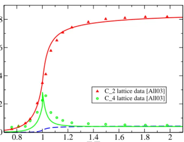
∆p(T, µ) T4 = 1 T4[p(T, µ)−p(T, µ= 0)] (4.1) ≡ ∞ X n=1 cn(T) µ T n . (4.2)
In [All03], the Taylor series in µ/T has been computed up to fourth order, i. e. c2
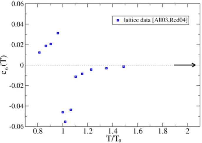
and c4 have been evaluated on the lattice. First partial results of c6 are published
in [All03, Red04].
The expansion coefficients cn(T) are directly calculable on the lattice for µ= 0.
They read cn(T) = Tn−4 n! ∂np ∂µn µ=0 . (4.3)
Using the QPM, the coefficients c