Inference in MCMC step selection models

White Rose Research Online URL for this paper:

http://eprints.whiterose.ac.uk/153402/

Version: Accepted Version

Article:

Michelot, T., Blackwell, P.G. orcid.org/0000-0002-3141-4914, Chamaillé Jammes, S. et al.

‐

(1 more author) (2019) Inference in MCMC step selection models. Biometrics. ISSN

0006-341X

https://doi.org/10.1111/biom.13170

This is the peer reviewed version of the following article: Michelot, T. , Blackwell, P. G.,

Chamaillé Jammes, S. and Matthiopoulos, J. (2019), Inference in MCMC step selection

‐

models. Biometrics, which has been published in final form at

https://doi.org/10.1111/biom.13170. This article may be used for non-commercial purposes

in accordance with Wiley Terms and Conditions for Use of Self-Archived Versions.

[email protected] https://eprints.whiterose.ac.uk/

Reuse

Items deposited in White Rose Research Online are protected by copyright, with all rights reserved unless indicated otherwise. They may be downloaded and/or printed for private study, or other acts as permitted by national copyright laws. The publisher or other rights holders may allow further reproduction and re-use of the full text version. This is indicated by the licence information on the White Rose Research Online record for the item.

Takedown

If you consider content in White Rose Research Online to be in breach of UK law, please notify us by

Inference in MCMC step selection models

Th´eo Michelot∗

Centre for Research into Ecological and Environmental Modelling, University of St Andrews, Buchanan Gardens, St Andrews KY169LZ, U.K.

*email:[email protected]

and

Paul G. Blackwell

School of Mathematics and Statistics,

University of Sheffield, Hounsfield Road, Sheffield S37RH, U.K.

and

Simon Chamaill´e-Jammes

CEFE, CNRS, Universit´e de Montpellier,

Universit´e Paul Val´ery Montpellier, EPHE, IRD, Montpellier, France

and

Jason Matthiopoulos

Institute of Biodiversity, Animal Health and Comparative Medicine, Graham Kerr Building, College of Medical, Veterinary and Life Sciences,

University of Glasgow, Glasgow G128QQ, U.K.

Summary: Habitat selection models are used in ecology to link the spatial distribution of animals to environmental covariates, and identify preferred habitats. The most widely used models of this type, resource selection functions, aim to capture the steady-state distribution of space use of the animal, but they assume independence between the observed locations of an animal. This is unrealistic when location data display temporal autocorrelation. The alternative approach of step selection functions embed habitat selection in a model of animal movement, to account for the autocorrelation. However, inferences from step selection functions depend on the underlying movement model, and they do not readily predict steady-state space use. We suggest an analogy between parameter updates and target distributions in Markov chain Monte Carlo (MCMC) algorithms, and step selection and steady-state distributions

000 0000

in movement ecology, leading to a step selection model with an explicit steady-state distribution. In this framework, we explain how maximum likelihood estimation can be used for simultaneous inference about movement and habitat selection. We describe the local Gibbs sampler, a novel rejection-free MCMC scheme, use it as the basis of a flexible class of animal movement models, and derive its likelihood function for several important special cases. In a simulation study, we verify that maximum likelihood estimation can recover all model parameters. We illustrate the application of the method with data from a zebra.

Key words: _{animal movement, local Gibbs sampler, Markov chain Monte Carlo, MCMC step selection, resource}

1. Introduction

Location data are routinely collected on animals, e.g. with GPS tags, resulting in bivariate

time series of coordinates. Statistical methods have been developed to combine location data

with environmental data, to understand how an animal’s use of space relates to the

distribu-tions of spatial covariates (e.g. vegetation type or resource density; see Manly et al., 2002).

A common focus of such analyses is habitat selection, i.e. deviations from proportionality

between habitat availability and habitat use by the animal (Northrup et al., 2013). Habitat

availability is derived from maps of the covariates, and habitat use from the location data. If

the time that the animal spends in different habitats is not proportional to their prevalence

in the study region, this suggests that it selects certain habitats over others, which is of great

interest for conservation.

In habitat selection studies, the goal is to estimate a habitat selection function

w

(c(x)),

which measures the strength of the selection for a habitat unit defined by the vector of

covariates

c(x) = (

c

(x)

, . . . , c

(x)) at spatial location

x. Habitat selection functions usually

take the form

w

{

c(x)

}

= exp

{

β

c(x)

}

,

(1)

where

β

= (

β

, . . . , β

) is a vector of unknown parameters. Each parameter

β

reflects the

effect of the covariate

c

on the animal’s use of space (i.e. apparent selection or avoidance).

Most commonly, the function

w

is called the “resource selection function” (RSF), and it is

interpreted as the long-term habitat selection by the animal (Boyce and McDonald, 1999).

The RSF is used to model the stationary distribution

π

(x) of the animal’s location in space,

termed the utilization distribution,

π

(x) =

R

w

{

c(x)

}

w

{

c(y)

}

d

y

(2)

where Ω denotes the study region. For example, if we consider a categorical habitat variable,

the utilization distribution

π

takes a different value over each habitat type. The utilization

distribution can be viewed as a heatmap of the animal’s usage of space, or as the probability

density for its location at an arbitrary time.

The coefficients

β

of the RSF link the utilization distribution to the distributions of

covariates. They can be estimated from location data, e.g. using a logistic regression for

use-availability data (Aarts et al., 2012). RSF models assume that the observed locations

are an independent sample from the utilization distribution, and they often ignore the

autocorrelation inherent in animal movement data (Fieberg et al., 2010). To define habitat

availability, RSF analyses typically assume that any location within the study area (e.g.

home range, population range) is equally accessible to the individual at each time step

(Matthiopoulos, 2003). However, ignoring the effect of movement can lead to

misinterpreta-tions, and the definition of the region of availability can have an impact on the estimated

selection parameters and utilization distribution (Beyer et al., 2010).

Alternatively, to address these limitations of RSFs, habitat selection can be defined through

a step selection function (SSF; Rhodes et al., 2005; Fortin et al., 2005), which measures

habitat selection at the time-scale of the individual observed movement steps. In an SSF

model, the likelihood of an animal moving from a location

x

to a location

y

is

p

(y

|

x) =

R

φ

(y

|

x)

w

{

c(y)

}

φ

(z

|

x)

w

{

c(z)

}

d

z

,

(3)

where

φ

(y

|

x) is the likelihood of a step from

x

to

y

in the absence of covariate effects,

which describes the underlying movement model. Matched conditional logistic regression is

typically used to estimate the parameters

β

of a SSF from telemetry data (Forester et al.,

2009). The autocorrelation of the data is explicitly accounted for, with this joint model of

animal movement and habitat selection. Habitat availability is specified by the movement

model, which describes which spatial units are accessible to the animal within one time step,

given its current location.

the regression coefficients

β

do not represent quite the same things in the two cases,

and the methods described do not lead to the same estimates of the coefficients, or of

the function

w

and the implied steady-state distribution. In an RSF, the coefficients are

directly linked to the global distribution

π

(x) of space use through Equation 2. However,

the coefficients of an SSF measure local habitat preference: their interpretation is tied to

the choice of the movement kernel

φ

. Unlike the RSF, the SSF therefore does not capture

the long-term utilization distribution. This discrepancy between the approaches has been

demonstrated analytically (Barnett and Moorcroft, 2008), and empirically (Signer et al.,

2017). The utilization distribution

π

is often of interest, and there have been efforts to derive

it from the SSF. In particular, for a generalization of the SSF model given in Equation 3, Potts

et al. (2014) described the evolution of the distribution of the animal’s location between times

t

and

t

+ 1. They iterated this calculation to evaluate the limiting utilization distribution

π

.

Alternatively, Signer et al. (2017) suggested using simulations from a fitted SSF to estimate

its stationary distribution. Although their approaches offer a way to numerically evaluate the

steady-state distribution of an SSF model, that distribution cannot be written as a simple

function of the spatial covariates (as in Equation 1).

Michelot et al. (2019) introduced a new model of step selection, in which both the

short-term movement rules and the long-short-term utilization distribution

π

arise from the same habitat

selection process. Here, we extend that approach to a much wider class of movement models.

We show how likelihood-based inference can be used to simultaneously estimate habitat

preference and movement characteristics from movement data, and present a simulation

study to investigate the performance of the method (in the online supplementary material).

Finally, we illustrate the application of our approach with the analysis of a movement track

of plains zebra (

Equus quagga

), and we discuss model selection and model checking in this

framework.

2. Animal movement models based on MCMC

2.1

MCMC step selection model

First, we briefly summarize the approach of Michelot et al. (2019). By construction, a Markov

chain Monte Carlo (MCMC) algorithm describes step selection rules, determined by the

transition kernel

p

(x

x

), such that the long-term distribution of

{

x

,

x

, . . .

}

is a given

distribution, termed the target distribution (Gilks et al., 1995). As such, it can be considered

as the basis for a model of animal movement: the transition kernel defines the movement rules

of the animal, and the target distribution is the utilization distribution

π

(i.e. the long-term

distribution of the animal’s space use). To link the animal’s movement to the distribution of

the covariates of interest, we model the utilization distribution with a (normalized) RSF, as

given in Equation 2. The resulting model describes an animal’s movement in response to its

environment, similarly to SSF models, but it explicitly delivers the utilization distribution

π

. We call it an “MCMC step selection model”.

The MCMC step selection model has two sets of parameters. The parameters of the

tran-sition kernel

p

(x

x

), i.e. the tuning parameters of the MCMC algorithm, are movement

parameters. The parameters of the target distribution

π

, i.e. the

β

in Equation 1, are

habitat selection parameters. Our goal is to estimate those parameters jointly from movement

and habitat data. Our approach provides a framework for joint inference about short-term

movement, habitat selection, and long-term space use by animals.

In this framework, the choice of the MCMC sampler determines the choice of a movement

model. Some MCMC algorithms may not provide a realistic description of animal movement,

if the transition kernel is a poor representation of the animal’s step selection rules. In the

following section, we extend the algorithm introduced by Michelot et al. (2019) to a much

more flexible family of movement models. The sampler that they described is a special case

of the algorithm presented here, but we keep the “local Gibbs” name that they coined.

2.2

The local Gibbs sampler

In the context of the approach proposed in Section 2.1, our aim is to define a flexible MCMC

algorithm, with transition rules that resemble the step selection process of an animal.

Fol-lowing this idea, the local Gibbs sampler uses local information about the target distribution

to take steps in its parameter space, similarly to an animal using local information about its

environment to choose where to move.

The local Gibbs algorithm for the target distribution

π

is defined as follows on the domain

Ω. We choose

φ

: Ω

→

R

the density function of a symmetric distribution, i.e. such that

∀

x

,

y

∈

Ω

, φ

(y

|

x) =

φ

(x

|

y). We start from

x

∈

Ω; then, for

t

= 1

,

2

, . . .

,

(1) Generate a point

µ

from

φ

(

·|

x

).

(2) Define the distribution ˜

π

on the domain Ω by

˜

π

(x) =

R

φ

(x

|

µ)

π

(x)

φ

(z

|

µ)

π

(z)

d

z

.

(3) Sample the next point

x

from ˜

π

.

At each iteration, ˜

π

represents the local information about the target distribution

π

over a

neighborhood of

x

defined by

φ

. The sampled points

{

x

,

x

, . . .

}

have

π

as their stationary

distribution. This is verified in Web Appendix A. The local Gibbs sampler is thus a valid

MCMC algorithm for any symmetric density

φ

, with target distribution

π

. Note that it is

a rejection-free sampler, as it does not need an acceptance-rejection step to preserve the

correct stationary distribution.

In the framework described in Section 2.1, the target distribution

π

can be written as a

normalized RSF, with parameters

β, and the local Gibbs sampler defines a model of animal

movement and habitat selection. The choice of the density

φ

determines the shape of the

movement kernel. In the following, we consider the case where

φ

is a parametric function,

and we explicitly denote it

φ

(

·|

x

,

θ), where

θ

is a vector of movement parameters. We discuss

two useful special cases of

φ

, the normal kernel model and the availability radius model, in

Section 2.3. The intermediate point

µ

sampled in step 1 of the local Gibbs algorithm does

not have a biological interpretation; it is a stepping stone in the construction of a valid

transition kernel.

In the general case, the step density of the model from

x

to

x

is given by the transition

kernel of the algorithm,

p

(x

|

x

,

β

,

θ) =

π

(x

)

Z

φ

(x

µ

,

θ)

φ

(µ

|

x

,

θ)

R

π

(z)

φ

(z

|

µ

,

θ)

d

z

d

µ

.

(4)

The steps of the derivation are similar to the proof of the detailed balance condition, given

in Web Appendix A. Note that, although the algorithm is rejection-free, the step density

p

(x

x

,

β

,

θ) is typically positive at the point

x

=

x

, and this model therefore does

not preclude movement steps of length zero. (See also the zero-inflated case below.)

In the absence of covariate effects (i.e. if

∀

x

∈

Ω

, π

(x) =

k

), each step is the sum of two

φ

-distributed increments, and we therefore call

φ

the half-step density of the model. The

habitat-independent movement kernel of the local Gibbs model is given by the convolution

p

(x

x

,

θ) =

R

µ∈Ω

φ

(x

µ

,

θ)

φ

(µ

|

x

,

θ)

d

µ.

In step 2 of the algorithm given above, the integral

R

z∈Ω

φ

(z

|

µ)

π

(z)

d

z

cannot generally be

evaluated analytically, unless the covariates follow a tractable parametric form. In practice,

we can use Monte Carlo integration to sample from the transition density, as follows. At

each iteration, a large number of points

{

z

,

z

, . . . ,

z

}

is sampled from

φ

(

·|

µ), and

x

is

selected from the

z

, with probabilities given by

π

(z

)

/

P

π

(z

). With this procedure, we

can simulate movement tracks on a given utilization distribution; see Web Appendix E for an

example. The local Gibbs algorithm would usually not be an interesting choice for the general

purpose of sampling from a probability distribution (e.g. in Bayesian inference). Indeed,

although there are no rejections, the numerical integration requires many evaluations of the

target distribution for each iteration, which renders the procedure more computationally

intensive than, say, standard Metropolis-Hastings sampling. In the following, we consider

the local Gibbs algorithm only for the purpose of modeling animal movement.

We discuss the links between the local Gibbs algorithm and conventional Gibbs sampling

in Web Appendix C. We explore relevant special cases of the local Gibbs model in Section

2.3, and present extensions in Section 2.4.

2.3

Special cases of the local Gibbs model

An interesting special case of the local Gibbs model is obtained when the half-step density

φ

is taken to be a bivariate (circular) normal density centered on the origin

x

. We will

call this formulation the normal kernel model. In the absence of covariate effects, if

φ

is a

normal distribution with variance

σ

I, where

I

is the 2

×

2 identity matrix, then the

habitat-independent movement kernel is also a normal distribution, with variance 2

σ

I

. In this case,

the distance between

x

and

x

(the “step length”) follows a Rayleigh distribution with

scale parameter

√

2

σ

. The parameter

σ

of this model can thus be linked to the speed of

movement of the animal. It also determines the extent of the region over which the animal

can perceive its habitat.

The model described by Michelot et al. (2019) is another special case of the local Gibbs

model. In their approach, the half-step density

φ

is uniform over a disc of radius

r

centered

on the origin. At each iteration, the point

µ

is sampled from a uniform distribution over

D

(x

), where

D

(x) denotes the disc of radius

r

and center

x. Then, the endpoint

x

is

sampled from

π

truncated to

D

(µ). We will refer to

r

as the “availability radius”, drawing

a parallel with the availability radius model of Rhodes et al. (2005). Figures 1(A) and (B)

show the shapes of the habitat-independent transition densities of the local Gibbs model

when the half-step density

φ

is normal, and when it is uniform on a disc, respectively. These

two examples illustrate the flexibility of the underlying movement model.

The local Gibbs model can also be extended to include a discrete component in the half-step

distribution. In particular, it would be possible to define a zero-inflated version of

φ

as the

combination of a continuous symmetric distribution and some probability mass at the origin.

This model would allow for steps of length zero with positive probability, corresponding to

time steps over which the animal does not move.

2.4

Mixture of local Gibbs steps

A mixture of MCMC algorithms, all with stationary distribution

π

, defines a valid MCMC

algorithm for

π

. Tierney (1994) calls these mixtures “hybrid” algorithms. In our application,

an MCMC movement model can be defined by a combination of several transition kernels.

We consider three hybrid algorithms, to extend the local Gibbs movement model.

2.4.1

Local Gibbs with random parameters.

An extension of the local Gibbs algorithm can

be obtained by considering that the parameters

θ

of the half-step density

φ

are themselves

random, and are drawn independently at each iteration from a probability distribution

p

(θ

|

ω). This results in a hierarchical model, formulated in terms of the hyperparameters

ω. In this case, the step density is obtained by integrating over

θ, and Equation 4 becomes

p

(x

x

,

β

,

ω) =

π

(x

)

Z

p

(θ

|

ω)

Z

φ

(x

|

µ

,

θ)

φ

(µ

|

x

,

θ)

R

π

(z)

φ

(z

|

µ

,

θ)

d

z

d

µ

d

θ

.

(5)

This extension is convenient to define more general movement models. For example, the

radius parameter

r

of the availability radius model of Michelot et al. (2019) could be

treated as random rather than fixed, to capture the variations in the scale of perception

and movement of an animal through time. The radius parameter takes positive values, and

could be modelled with a gamma distribution with shape parameter

α

and rate parameter

ρ

. In this example,

θ

=

r

,

ω

= (

α, ρ

), and

p

(θ

|

ω) is the gamma pdf. Figure 1(C) shows the

habitat-independent step density of this random availability radius model.

2.4.2

State-switching local Gibbs model.

The local Gibbs model has two sets of

param-eters: the parameters

β

of the utilization distribution

π

, and the movement parameters

θ

of the half-step density

φ

. For example, the movement parameters are the variance

σ

in

the normal kernel model, and the availability radius

r

in the availability radius model. This

framework can be extended by considering that the animal switches between

N

discrete

states through time, each associated with a set of movement parameters

{

θ

, . . . ,

θ

}

. We

can model the switching behavior with a latent process (

S

) defined on

{

1

, . . . , N

}

, which

indicates which state is active at each time step

t

(e.g. a Markov chain). Multistate models

like this one are very popular in movement ecology, to describe animal movement as the

consequence of behavior. The states are usually treated as proxies for behavioral states of

the animal, such as “foraging” or “exploring” (Blackwell, 1997, 2003; Morales et al., 2004).

The target distribution of the local Gibbs sampler does not depend on the movement

parameters

θ. It only depends on the habitat selection parameters

β. In this multistate

formulation, the movement process switches between

N

local Gibbs models, all with the

same parameters

β

and utilization distribution

π

. The utilization distribution of the

state-switching model is therefore also

π

. The underlying MCMC algorithm can be seen as a hybrid

algorithm, based on

N

transition kernels.

Roever et al. (2014) showed that ignoring animal behavior in habitat selection studies could

lead to incorrect conclusions. They argued for a two-stage modeling approach, in which tracks

would first be classified into behavioral states using a state-switching correlated random

walk model (Morales et al., 2004), and a separate set of habitat selection parameters would

then be estimated for each behavioral state. The state-switching local Gibbs model that we

suggest here is different, because it estimates only one set of habitat selection parameters

for all states. This is a limitation of our approach, because the habitat selection cannot

be estimated separately in the different states, and the estimated parameters may capture

the averaged effects of habitat selection over all behavioral states. However, the scale of

perception and movement can differ among the states, if they are characterized by different

parameters

θ

. Then, the state-switching local Gibbs model does account for the behavioral

heterogeneity in the scale of habitat selection.

2.4.3

Local Gibbs over irregular intervals.

A movement model based on an MCMC

algo-rithm is generally formulated in discrete time, where a time step of the model corresponds

to an iteration of the algorithm. This is in particular true of the local Gibbs sampler: the

parameters of the half-step density are tied to a particular time scale. We can relax this

constraint, by making an assumption on the relationship between the time interval and the

scale of the half-step density. In this section, we consider irregular time points (

t

, . . . , t

),

and the corresponding locations

x

=

x

,

j

= 1

, . . . , n

.

There is no general scaling property for the parameters of the half-step density, but we can

use the assumptions of Brownian motion to express this time dependence in the special case

of the normal kernel model. The variance of the transition density of the Brownian motion

is proportional to the length of the time interval (Einstein, 1905). Based on this assumption,

we consider the local Gibbs model with half-step density

φ

(

·|

x

) =

ϕ

(

·|

x

,

∆

σ

I

), where

ϕ

is the normal pdf, ∆

=

t

−

t

is the length of the time interval, and

I

is the identity

matrix. The step density of this model can thus be written

p

(x

|

x

) =

π

(x

)

Z

ϕ

(x

|

µ

,

∆

σ

I

)

ϕ

(µ

|

x

,

∆

σ

I)

R

π

(z)

ϕ

(z

|

µ

,

∆

σ

I)

d

z

d

µ

.

(6)

In the absence of covariate effects, the step density between

t

and

t

is

p

(x

x

) =

ϕ

(x

x

,

2∆

σ

I

), the transition density of the Brownian motion with diffusion rate 2

σ

.

This can be viewed as a hybrid algorithm, with the transition kernel changing as a function

of the time interval. This formulation can be used to model movement data collected at

irregular time intervals, because the scale parameter

σ

is not tied to a particular discrete

time step.

3. Inference

The parameters of an MCMC step selection model can be estimated, to carry out inference

about the effects of environmental covariates on the animal’s movement and space use.

3.1

The local Gibbs likelihood

In the local Gibbs model, our aim is to estimate the habitat selection parameters

β

(pa-rameters of the utilization distribution

π

), and the movement parameters

θ

(parameters

of the half-step density

φ

), from observed animal movement and habitat data. In the

fol-lowing, we consider

T

locations

x

, . . . ,

x

, observed without measurement error. The

like-lihood of a step from

x

to

x

, under the local Gibbs model, is given by the

transi-tion kernel

p

(x

x

,

β

,

θ) of the algorithm (Equation 4) and, for

T

observed locations,

the full likelihood is obtained as the product over observed steps,

L

(β

,

θ

|

x

, . . . ,

x

) =

Q

t=1

p

(x

x

,

β

,

θ). Estimates of the model parameters can be obtained by maximizing

the likelihood with respect to

β

and

θ, as here, or by using it in a Bayesian framework.

The likelihood of a step under the normal kernel and the availability radius models,

presented in Section 2.3, can be derived by substituting the corresponding expressions of

the half-step density

φ

in the transition kernel of Equation 4. Similarly, for the local Gibbs

model with random parameters and the local Gibbs model with irregular intervals, the

likelihood is given by the step densities derived in Sections 2.4.1 and 2.4.3, respectively. In

Web Appendix B, we present the derivation of the likelihood for the models considered in

the simulation studies and analyses of the next sections.

In this framework, it is straightforward to account for missing location data in the

like-lihood: missing steps (i.e. with missing start point or end point) have no contribution. If

several independent movement tracks are collected, possibly on several different animals,

their joint likelihood may be calculated as the product of the likelihoods of the individual

tracks, to obtain pooled parameter estimates.

Likelihood-based model selection criteria, such as the AIC and BIC, can be derived to

com-pare competing MCMC movement model formulations. In Section 4, we suggest predictive

checks to assess goodness-of-fit for the local Gibbs model.

3.2

State-switching local Gibbs model

In the state-switching model presented in Section 2.4.2, the parameters of the half-step

density

φ

can take

N

values

{

θ

, . . . ,

θ

}

. An underlying state process (

S

t

) determines

which of the

N

densities is active at each time step

t

. If (

S

) is chosen to be a Markov chain,

this defines a hidden Markov model, and the associated inferential machinery can be used:

the likelihood can be calculated with the forward algorithm, which provides an efficient way

to sum over all possible state sequences (Zucchini et al., 2016). In the present context, it

can be written

L

(β

,

{

θ

}|

x

1

, . . . ,

x

) =

δ

P

(x

,

x

)

Γ

P

(x

,

x

)

· · ·

Γ

P

(x

,

x

)

1

, where

δ

is the initial distribution of the Markov chain,

Γ

= (

γ

)

is its transition probability

matrix,

P

(x

,

x

) is the

N

×

N

diagonal matrix with elements

{

p

(x

|

x

,

β

,

θ

)

}

,

and

1

is a

N

-vector of ones. Maximum likelihood can be used to obtain estimates of all

model parameters, including habitat selection parameters (β), movement parameters (θ

),

and transition probabilities (

Γ

). The Viterbi algorithm can be implemented to derive the

most likely sequence of underlying states, given the data and a fitted model (Zucchini et al.,

2016). This approach is used in animal movement analyses to classify observed locations into

behavioral phases, described by different movement characteristics (Michelot et al., 2016).

3.3

Monte Carlo approximation of the likelihood

The integrals in the likelihood expression given in Equation 4 cannot generally be evaluated

analytically. Monte Carlo sampling can be used as follows to approximate the likelihood of

a step from

x

to

x

.

For

i

∈ {

1

, . . . , n

}

, sample

µ

from

φ

(

·|

x

,

θ) and for

j

∈ {

1

, . . . , n

}

sample

z

from

approximated by

ˆ

p

(x

|

x

,

β

,

θ) =

π

(x

)

n

n

X

φ

(x

|

µ

,

θ)

P

π

(z

)

.

(7)

In the case where

θ

is random, the likelihood is written with one additional integral

(Equation 5), which must also be approximated. As an example, the approximate likelihood

of the random availability radius model is given in Web Appendix D.

The approximation in Equation 7 can be made arbitrarily accurate by choosing large sizes

of Monte Carlo samples (

n

and

n

). Latin hypercube sampling can be used to reduce the

number of samples needed in the approximation of the likelihood (McKay et al., 1979). In

Web Appendix D, we describe the practical implementation of the local Gibbs approximate

likelihood for the normal kernel model and the random availability radius model.

In Web Appendix E, we investigate the performance of the method to estimate the RSF

and the movement parameters from simulated movement data. The simulations confirm

that all model parameters can be recovered, by numerical optimization of the approximate

likelihood.

4. Application: zebra case study

We consider a track of GPS locations of one plains zebra, acquired every 30 minutes from

January to May 2014 in Hwange National Park (Zimbabwe). The track consists of 7246

locations, regularly spaced in time, with 125 missing observations. The habitat layer used to

estimate the habitat selection process is a vegetation map, with four categories: grassland,

bushed grassland, bushland, and woodland. A map of the habitat and of the track is shown

in Figure 2(A). The code and data used in the case study are provided in the supplementary

material.

4.1

Normal kernel model

We fitted the local Gibbs model with normal half-step density to the track, using the function

optim

in R to numerically optimize the (approximate) log-likelihood function. We chose

n

=

n

= 50 for the Monte Carlo samples in the approximation of the likelihood function

(Equation 7), which was sufficient in the simulation study of Web Appendix E.

A numerical optimizer is susceptible to becoming stuck in a local maximum of the likelihood

function, and failing to find its global maximum. To circumvent this problem, we fitted the

model 50 times, starting from randomly-chosen initial parameter values, and we selected the

parameter estimates leading to the best (largest) maximum likelihood. Each model fit took

about 8 minutes on a 2GHz i5 CPU. For the best fitting model, we numerically evaluated

the Hessian matrix of the log-likelihood function at the maximum likelihood estimate, and

we derived standard errors for the estimated parameters.

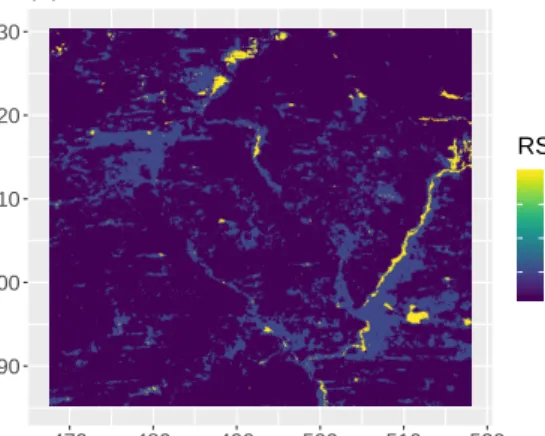
The estimates of the habitat selection parameters and the Hessian-based (Wald) 95%

confidence intervals are given in Table 1 (under “Model 1”), and a map of the fitted RSF is

shown in Figure 2(B). The estimated habitat selection parameters indicate that this zebra

selects open habitats more strongly than wooded areas, which is consistent with the natural

history of the species. Zebras prefer more open areas that provide more forage and greater

visibility. This result is also consistent with an analysis based on a standard RSF, conducted

by Courbin et al. (2016) on many individuals in the same area, albeit with a different

vegetation map.

[Table 1 about here.]

[Figure 2 about here.]

The standard deviation of the half-step density was estimated to ˆ

σ

= 0

.

20. Under this

model, in the absence of covariate effects (e.g. in a large patch of uniform habitat), the step

lengths of the animal follow a Rayleigh distribution with scale parameter

λ

=

√

2

σ

. The

estimate of the scale parameter is ˆ

λ

= 0

.

28, and the mean of the (habitat-independent) step

length distribution can be derived as

p

π/

2ˆ

λ

= 0

.

35km. This gives an estimate of the scale

of movement and perception of the zebra over 30 min time intervals.

To assess this movement model, we simulated 10

locations from the fitted model, on the

same habitat map as the observations. We compared the distribution of step lengths observed

in the zebra data set to the distribution of simulated step lengths (Figure 3). There is a clear

discrepancy between the two distributions: the model fails to capture very short and very

long step lengths, and overestimates the density of intermediate step lengths. The empirical

distribution of step lengths has a mode at zero, and a long tail, which cannot be appropriately

modelled by this formulation. We then considered the random availability radius model for

more flexibility.

4.2

Random availability radius model

We fitted the local Gibbs model with random availability radius, described in Section 2.4.1,

to the same track. We modelled the availability radius with a gamma distribution, and

estimated its shape and rate parameters. We used Monte Carlo samples of sizes

n

= 20 and

n

=

n

= 40, following the simulation study of Web Appendix E. As in Section 4.1, we

ran the numerical optimization 50 times with random initial parameter values, and kept the

model fit with the largest likelihood, to avoid numerical convergence issues. Each model fit

took about 1.5 hour on a 2GHz i5 CPU. We evaluated the Hessian matrix of the log-likelihood

at the maximum likelihood estimates, and derived standard errors for the parameters.

The estimates of the habitat selection parameters, and the 95% confidence intervals, are

given in Table 1 (under “Model 2”), and a map of the RSF is shown in Web Appendix I.

The parameter values are quite similar to those obtained with the normal kernel model, and

the results confirm that the selection is stronger for open habitats (i.e. grassland and bushed

grassland). The estimated shape of the gamma distribution of the availability radius was

ˆ

α

= 0

.

78, and the rate was ˆ

ρ

= 3

.

57. The estimated gamma distribution of the availability

radius therefore had mean ˆ

E

(

r

) = ˆ

α/

ρ

ˆ

= 0

.

22km, and 95th percentile ˆ

P

= 0

.

72km, for

30 min intervals.

To assess the random availability radius model, we simulated a track of length 10

from

the fitted model, on the same habitat map. We compared the distributions of observed and

simulated step lengths (Figure 3). The distribution of the simulated steps resembles that of

the observed steps much more closely than with the normal kernel model. This indicates that

the model was able to capture the speed of the zebra’s movement. This is remarkable, as the

step lengths or the speeds are never directly modelled: instead, we estimated the distribution

of the unobserved radius of the relocation region.

[Figure 3 about here.]

There is a trade-off between realism of the movement model and computational speed: the

random availability radius model was 15-20 times slower than the normal kernel model in

this analysis, due to the additional nested integral in its likelihood (Equation 5). Here, the

habitat selection estimates ˆ

β

were very similar using both models. This suggests that the

simpler one (normal kernel model) is sufficient to capture the RSF, even if the movement

component is not flexible enough to capture the zebra’s step lengths. However, we could not

have known this before fitting the random availability radius model and, generally, model

checking methods should be used to verify that features of the movement are appropriately

captured by the model. In this analysis, the AIC for the normal kernel model was

−

141, and

the AIC for the random availability radius model was

−

8906. This criterion thus strongly

favored the latter, more complex, model.

In the local Gibbs algorithm, the half-step density

φ

is required to be symmetric, to

satisfy the detailed balance condition (Section 2.2). As a consequence, the local Gibbs model

does not include directional persistence. This can be a problem to analyse high-resolution

movement data, which typically feature strong persistence. To investigate the effect of this

misspecification on the estimates of the habitat selection parameters, we fitted the normal

kernel model to data simulated from a step selection model with directional persistence. The

simulations are presented in Web Appendix H. We found that, for moderately persistent

movement (similar to the zebra’s), the local Gibbs model could still accurately recover the

utilization distribution. However, for simulated data with strongly autocorrelated directions,

the estimates of habitat preference were biased. This suggests that the local Gibbs model may

not be appropriate to analyse very persistent movement, e.g. collected at a high temporal

resolution.

5. Discussion

We showed how a new class of step selection models, based on the same underlying concept

as MCMC algorithms, can be used to estimate an animal’s habitat selection and movement

characteristics. In this framework, short-term step selection gives rise to the long-term

utilization distribution. This approach connects standard RSF and SSF models, because

the equilibrium distribution of the movement model is guaranteed to be proportional to the

underlying RSF. We described maximum likelihood estimation for the local Gibbs sampler,

a flexible family of MCMC algorithms which can be used to model animal movement.

Parameters of movement and habitat selection can be estimated jointly.

In the case study of Section 4, we compared two local Gibbs models with different half-step

densities, and we found a trade-off between the flexibility of the movement model and the

computational cost of inference. Our framework is not limited to the special cases described

here, however, and it may be possible to find a local Gibbs formulation that combines the

computational speed of the normal kernel model and the flexibility of the random availability

radius model. For example, we could define the half-step density

φ

as the combination of

a uniform distribution of turning angles and a given distribution for the distance to the

origin. The uniform angles ensure that the half-step density is symmetric, and the shape of

the distance distribution determines the habitat-independent movement model. It may be

possible to achieve a distribution of step lengths with a mode close to zero, as in the zebra

data set, with an exponential or Weibull distribution of distances.

An important feature of the local Gibbs model is that the size of the region of availability

does not need to be defined a priori. In habitat selection analyses based on use-availability

designs, the choice of the spatial extent of the availability region is challenging, and can lead

to biased selection estimates (Beyer et al., 2010). Instead of choosing it, we estimate it from

the observed tracking data, with a movement model based on a symmetric half-step density.

The scale of availability is for example measured by the variance of the normal kernel model,

and by the radius in the availability radius model. One limitation of this method is that the

scale of availability jointly captures the accessibility and the local information that the animal

has about the habitat (e.g. through perception, memory, shared information). The half-step

density of the algorithm therefore describes both the distance that the animal is likely to

cover over one time interval, and the size of the region over which it knows the habitat. This

is a strong assumption, that is made in most step selection models (Forester et al., 2009),

in which habitat selection is considered to take place at the scale of the movement kernel.

Recently, Avgar et al. (2015) and Bastille-Rousseau et al. (2018) have proposed models to

estimate the movement process and the perception on separate scales. Additional work is

required to allow this flexibility within the framework presented in this paper.

Acknowledgements

We are grateful to Jonathan Potts and Otso Ovaskainen for discussions about this work,

and to the associate editor and two reviewers, for their helpful suggestions. TM was funded

by the Leverhulme Trust, award number DS-2014-081. SCJ was supported by the grant

ANR-16-CE02-0001-01 of the French

Agence Nationale de la Recherche

.

References

Aarts, G., Fieberg, J., and Matthiopoulos, J. (2012). Comparative interpretation of count,

presence–absence and point methods for species distribution models.

Methods in Ecology

and Evolution

3,

177–187.

Avgar, T., Baker, J. A., Brown, G. S., Hagens, J. S., Kittle, A. M., Mallon, E. E., McGreer,

M. T., Mosser, A., Newmaster, S. G., Patterson, B. R., et al. (2015). Space-use behaviour

of woodland caribou based on a cognitive movement model.

Journal of Animal Ecology

84,

1059–1070.

Barnett, A. H. and Moorcroft, P. R. (2008). Analytic steady-state space use patterns and

rapid computations in mechanistic home range analysis.

Journal of mathematical biology

57,

139–159.

Bastille-Rousseau, G., Murray, D. L., Schaefer, J. A., Lewis, M. A., Mahoney, S. P., and Potts,

J. R. (2018). Spatial scales of habitat selection decisions: implications for telemetry-based

movement modelling.

Ecography

41,

437–443.

Beyer, H. L., Haydon, D. T., Morales, J. M., Frair, J. L., Hebblewhite, M., Mitchell, M.,

and Matthiopoulos, J. (2010). The interpretation of habitat preference metrics under

use–availability designs.

Philosophical Transactions of the Royal Society of London B:

Biological Sciences

365,

2245–2254.

Blackwell, P. (1997). Random diffusion models for animal movement.

Ecological Modelling

100,

87–102.

Blackwell, P. G. (2003). Bayesian inference for Markov processes with diffusion and discrete

components.

Biometrika

90,

613–627.

Boyce, M. S. and McDonald, L. L. (1999). Relating populations to habitats using resource

selection functions.

Trends in Ecology & Evolution

14,

268–272.

Chamaill´e-Jammes, S. (2016). Reactive responses of zebras to lion encounters shape

their predator–prey space game at large scale.

Oikos

125,

829–838.

Einstein, A. (1905). ¨

Uber die von der molekularkinetischen Theorie der W¨arme geforderte

Bewegung von in ruhenden Fl¨

ussigkeiten suspendierten Teilchen.

Annalen der Physik

322,

549–560.

Fieberg, J., Matthiopoulos, J., Hebblewhite, M., Boyce, M. S., and Frair, J. L. (2010).

Correlation and studies of habitat selection: problem, red herring or opportunity?

Philosophical Transactions of the Royal Society of London B: Biological Sciences

365,

2233–2244.

Forester, J. D., Im, H. K., and Rathouz, P. J. (2009). Accounting for animal movement

in estimation of resource selection functions: sampling and data analysis.

Ecology

90,

3554–3565.

Fortin, D., Beyer, H. L., Boyce, M. S., Smith, D. W., Duchesne, T., and Mao, J. S.

(2005). Wolves influence elk movements: behavior shapes a trophic cascade in yellowstone

national park.

Ecology

86,

1320–1330.

Gilks, W. R., Richardson, S., and Spiegelhalter, D. (1995).

Markov chain Monte Carlo in

practice

. CRC press.

Manly, B., McDonald, L., Thomas, D., McDonald, T. L., and Erickson, W. P. (2002).

Resource selection by animals: statistical design and analysis for field studies, Second

Edition

. Kluwer Academic Publishers, Dordrecht.

Matthiopoulos, J. (2003). The use of space by animals as a function of accessibility and

preference.

Ecological Modelling

159,

239–268.

McKay, M. D., Beckman, R. J., and Conover, W. J. (1979). Comparison of three methods

for selecting values of input variables in the analysis of output from a computer code.

Technometrics

21,

239–245.

Michelot, T., Blackwell, P. G., and Matthiopoulos, J. (2019). Linking resource selection and

step selection models for habitat preferences in animals.

Ecology

100,

e02452.

Michelot, T., Langrock, R., and Patterson, T. A. (2016). moveHMM: An R package for the

statistical modelling of animal movement data using hidden Markov models.

Methods in

Ecology and Evolution

7,

1308–1315.

Morales, J. M., Haydon, D. T., Frair, J., Holsinger, K. E., and Fryxell, J. M. (2004).

Extracting more out of relocation data: building movement models as mixtures of random

walks.

Ecology

85,

2436–2445.

Northrup, J. M., Hooten, M. B., Anderson, C. R., and Wittemyer, G. (2013). Practical

guidance on characterizing availability in resource selection functions under a use–

availability design.

Ecology

94,

1456–1463.

Potts, J. R., Bastille-Rousseau, G., Murray, D. L., Schaefer, J. A., and Lewis, M. A. (2014).

Predicting local and non-local effects of resources on animal space use using a mechanistic

step selection model.

Methods in Ecology and Evolution

5,

253–262.

Rhodes, J. R., McAlpine, C. A., Lunney, D., and Possingham, H. P. (2005). A spatially

explicit habitat selection model incorporating home range behavior.

Ecology

86,

1199–

1205.

Roever, C. L., Beyer, H., Chase, M., and Van Aarde, R. J. (2014). The pitfalls of ignoring

behaviour when quantifying habitat selection.

Diversity and Distributions

20,

322–333.

Signer, J., Fieberg, J., and Avgar, T. (2017). Estimating utilization distributions from fitted

step-selection functions.

Ecosphere

8,

.

Tierney, L. (1994). Markov chains for exploring posterior distributions.

The Annals of

Statistics

22,

1701–1728.

Zucchini, W., MacDonald, I. L., and Langrock, R. (2016).

Hidden Markov models for time

series: an introduction using R, Second Edition

. Chapman and Hall/CRC.

Supporting information

Web Appendices referenced in Sections 2, 3 and 4 are available with this paper at the

Biometrics website on Wiley Online Library. The code and data used in the simulation

studies and the case study are available in the online supplementary material.

(A) x coordinate 0 Step density (B) x coordinate −2r 0 2r Step density (C) x coordinate 0 Step density

Figure 1.

Slices through the two-dimensional habitat-independent step densities in three

different MCMC movement models. (The step densities are symmetric around the origin.)

(A) Normal kernel model. (B) Availability radius model. (C) Availability radius model,

with time-varying radius

r

drawn from a gamma distribution. Analytical formulas can be

● ●●●●●●●●●●● ●●●●●●●●●●●●●●●●●● ●●●●●● ●●●●●●●●●●●●● ●●●● ●●●●●●●●● ●●●●●● ● ● ● ●●●●● ● ● ●●●●●● ●●● ● ●●●●●●●●●●●●●●●●●●●●●●●●●●●●● ●● ●●●●●●●●● ●● ● ●●● ● ●● ● ●● ●●●●●● ●●● ●●● ●●●●●● ●● ● ●●●●●● ●● ●●●●●●● ●●●●●●●●●● ●●●●●● ●●●●●●●●●●●●● ● ●●●● ● ●●●●●●●●●●● ●●●●● ● ●●● ●●●●●●●●●●●● ● ● ●●●● ● ● ● ● ●●●● ● ● ● ● ● ● ● ●● ● ●● ●●● ● ● ● ● ● ●●●●●●●● ● ● ●●●●●●●●●●●●●●●●●●●●●●●●●●●●● ●●●●● ●● ●●●● ● ● ●● ●●●● ●● ● ● ●●●●●● ●● ● ●●●●●●●●●●●●●●●●●● ● ●●● ●●●●● ● ●●● ●●●●●●●●●●●●●●●● ● ●●● ●●●●●● ●●●●●●●●●●●●●●●●●●●●●●●●●●●●●●●●●●●●●●●●●●●●●●●●●●●●●●● ●●● ● ● ●●●●●●●●●●●●●●●●●● ●●●●● ● ● ● ●●●●●● ●●●●●●●●●●● ●●●●●●●● ●● ● ● ●●●● ●●●●●●●●●●●●●● ● ● ●●●●●●●●●●●●●●●●●●● ● ● ● ●●● ● ● ● ● ● ● ● ● ●●● ●●●●● ●●●●● ●● ● ●●●●● ● ●●●●● ● ●●●●●●●●● ● ● ● ●●●●●● ●●●●●●●●●●●●●●● ●●● ●●●●●●●●●●●●●●● ●●●●●●●●●● ●●●●●●●●●● ●●●●●●●●●●●●●●●● ●●●●●●●●● ● ●●●●●●●● ●●●●●●●●● ●●●●●●● ●●●● ●●●●●●●●●●●●●●●●● ● ●●●●●●● ● ●●●●●● ●●●●●●●●●●●●●●●●● ●●●● ●●● ●●● ● ●●●●●●● ●●●●●● ●●●●●●●●●●●●●●●●●●●●●●●●●●●●●●●●●●●●●●●●●●●● ●●●●●●●●●●●●●●●●● ● ● ● ● ● ● ● ● ● ● ● ● ● ● ●●●●● ●●●●● ● ● ● ●●●●●●●●●●●●●● ●●●●●●●● ●● ● ● ● ● ● ● ● ● ● ● ● ● ●●●●●● ●●●●●● ● ● ● ● ● ●● ●● ● ●●● ●● ●● ● ● ●● ●● ●●●●●●● ●●●●●●●●●●●●●●●●●●●● ● ●● ●● ● ● ●●●●●●●●●●●●●●●●●●●●●●● ● ●●●●●●● ● ●●●●● ●●●● ●●●●● ●● ●● ● ● ●● ●●●●●●●●●●●● ●●●●● ●● ●●●●● ● ●● ●●● ● ● ● ● ● ●●● ● ● ● ●●●●● ●●●●●●●●● ●●●●●●●● ●●●●●●●●●●●●●●●●●●●●●● ●● ● ● ●●●●●●●●●●●●●●● ●●●●●● ●●●●●●● ●●● ● ●● ● ●●●● ● ● ●● ●●● ● ●●●●●●● ● ●●●●●● ●●● ● ●●●● ● ●● ●●●●●●●●● ● ●●●●● ● ●●●● ● ●●●●●●●●●●●●●●●●●●●●●●●●●●● ● ● ●● ●●●●●●●●●●●●●●●●●●●●●●●●●●●●●●●●●●●●●●●●●●●●●●●●●●●●●●●●●●●●●●●●●●●●●●●●●●●●●●●●●●●●●●●●●●●●●●●●●●●●●●●●●●●●●●●●● ● ● ●●●● ●●● ● ● ● ●●● ●●●●● ●● ● ●●●●● ●●●●●●●●●●●●●●●●●●●●●●●●●● ●● ●● ●●●●●●● ● ● ● ●● ● ● ● ● ● ●● ●●● ●●●●● ●● ● ● ● ●●●●●● ● ●●●●●●●●●●●● ●●●●● ●● ●● ●● ●●●●●●●●● ● ●●●●●●●●●●●●●●●●●●●●●●●●●● ● ● ● ● ●●●●● ●●●●●●● ●● ●●●●●● ● ●●●●●● ●●●● ●● ●●●●●●●●●● ●●●●●●● ●●●●●●●●●●● ●●●●●●●●●●●●●●●●●●●●●●●●●●●●●● ●● ● ●●● ● ●●●●●●●●●●●●●●●●●● ●●●●●●●●●●●●●●●●●●●●●●●●● ●●●●●●●●●●●●● ●●●●● ●●●●●●● ●●●●● ●●●● ●●●●●●●●●●●●●●●●●●● ●●● ●●● ● ●●● ● ●●●● ● ● ● ● ● ●●●●●●● ●●●●●●●● ●●●●●●●●● ● ●●●●●●●●● ●●●●●●● ●●● ● ● ● ●●● ●●●●● ● ●●●●● ● ●●●●●●●● ● ● ●●● ● ●●●●●●●●●●●●● ●●●● ● ●●●●● ●● ●● ●● ●●●●● ●●●●●●●●●● ●●●●●● ● ● ●●●●●●● ● ●●●● ● ●● ● ●●● ●● ●● ● ●●●●●●●●●●●●●●●● ● ●●●● ● ●●●●●●● ● ●● ● ●● ● ● ● ● ● ●●●●● ●●●●●●●●●●●●● ●●●● ●●●●●●●●●●●●●● ●●● ● ● ● ● ● ●●●● ● ●● ● ● ● ●●● ● ● ● ●● ● ●●● ● ● ●●●●●●●●●●●●●● ●●●●● ●● ● ●●●●●●●●● ●● ● ● ● ●● ●● ●●●●●●● ●●●●● ● ●● ●●●●●●●●●●●●●●● ●● ● ● ● ●●●● ● ●●●●●●●●●●● ●●● ● ●●● ●●●●●●●●● ● ● ●● ●● ●●● ● ●●●●●●●●●●●●●●●●●●●●●● ● ●●●●●●●●●●●●● ●●● ●●●●●●● ●● ●●●●●●●● ●●●●● ●●●● ●●●●●●●●● ●●●●●●●●●●●●●●●●●●●●● ●●●●●●●●● ●●●●●●●●●●●●●●●●● ●●●● ●●● ● ● ● ● ● ●● ● ● ● ● ● ● ● ● ● ●●●●●●●●●● ●●●●●●●●●●●● ●● ●●● ● ●●●●●●● ●●●●●●●●●● ●● ● ● ● ●●● ● ●● ●● ●● ●●●● ●●●● ●●●●●●● ● ● ● ●●●●●●●●●●● ●● ● ●●● ●● ●●●●● ●●●●●●●●●● ●●●●●●●●●●●●●●●●●●●●●●●●●● ●●●●● ● ●● ●●●●●●●●●●●●●●●●●●●●●●●●●●● ●● ● ● ● ● ● ● ● ● ● ●●●●●●●● ● ● ●●●●●●●●●●●●●● ●●●●●●●●●●●● ● ● ● ●● ● ●● ● ● ●● ●● ● ● ●● ● ● ● ● ●● ● ●● ●●●●●●●●●●●●●●●● ● ● ●●● ●●●●● ● ● ●●●●● ● ● ●● ●●● ●● ●●●●● ●●●●● ●●●●● ●●●●●●●●● ●●●●●●●●●●●●●●●●●●●●● ●●● ●●●●●●●●●●●●● ● ●●●●● ● ● ● ●● ● ● ● ●● ● ● ● ●●●●●●●●● ● ●●●● ●●●●●●●●●●●●●●●●●●●●●●●●●●●●●●●●●●●●●● ●●● ●● ●●●●●● ● ● ●●●●●●● ●●●●●●●●●●●●●●●●●●●●● ● ●●●●●●●●●●● ● ●●●●●●●●●●●●●●●●●●●●●●●●●●●●●●●●●●●●●● ●●●●●●●●●●●●●●● ● ●●● ●●●● ●●●●●● ●●●●●●●●●●●●●●●●●●●●●●●●● ●●●●●●●●●●●●●●●●●●● ● ● ● ●●●●● ● ●●●●●●●●●● ● ● ●●●●●●●●●● ●●● ● ● ● ●●●●●●●●●●●●●●●●●●●●●●●●●●●● ●●●●●● ●●●●●● ●● ●● ●●● ● ● ●●●●●●●●●●●●●●●●●●●●● ●●●●●●●●●●●● ● ● ● ● ●●●●●●●● ●●●●●●●●●●●●●●●●●●●●●●●●●●●●●●● ●●●●●●●●●●●●●●●● ●●●●●●●●●●●●●●●●● ● ● ● ● ●● ●●●● ● ● ● ● ● ●●● ●●●●●●● ●● ●●● ● ● ●● ● ● ● ● ● ●●●●●●●●●●●●●●●●●●●●● ● ● ● ● ● ●● ●●●● ● ●●●●●●●●●● ●●●●●●●● ●●●●● ● ● ●●●● ●●●●●●●●●●●● ●●●● ●●● ● ●●●●●●●●● ● ●●●●●●●● ●●●●●●●●●●●●●● ●●●●● ●●●● ●●● ●●●●●●●●●●●●● ● ●●●●●●●●●●●●●●●● ●●●●●●●●●●●●●●●●●●●●●●●●●●● ●●●● ● ● ● ● ●●●●● ●●●●●●● ●●●●●● ●●●● ● ● ● ● ●●●●●●●●●●●●●●●●●● ● ●●● ●●● ●●●●●●● ●●●●●●●●● ●● ●●●● ●●●●●●●● ●●●●●●● ●●●●●●●●●●●●●●●● ●●●●●● ●●●●●●●●●●●●● ●● ●●●●●●●●●●●●●● ●●●●● ● ●●●●●●●●●● ●●●●●●●●●● ● ●● ●● ●●●●●●●●●●●●●●●● ●●●●●●●●●●●●● ● ●●●●●● ●●●●●●●●●●●●●● ● ●● ●● ●●●●● ●●●●●●● ●●●●●● ● ●●●●●●●●●●●●●●●●●●●●●●●●●●●●●●●●●●●●●●●●● ● ● ●●● ● ●●● ● ● ● ●● ●● ● ●●● ● ● ●●●●●●●●●●●●●●●●●● ● ●● ● ● ●● ● ●●●●● ●●●●●●●●●●●●●●●●●●●●●●●●● ●●●●●●●● ● ● ● ●●●●● ●● ●●●● ●●●●●●●● ●●●●●●●●●●● ●● ●●●●● ●● ●● ● ● ● ● ●●●●●●●●● ●●●●●●●●● ● ●●●●● ● ● ●●●●●●●● ● ●●●●●●●●●●●●●●●●●●●● ●●●●●●●●●●●● ●●●●●●●●●●●● ●●●●●●●●● ●●●● ●● ●● ●●● ●●●●●●●●●●● ● ●● ● ●●●●● ● ● ●●●●●●●●●●●●●●●●●●●●●●●●●● ● ●●● ●●● ● ● ● ●●● ●●●●●●●●●●●●●●●●●● ● ● ● ●● ● ● ● ● ●● ● ●● ●●●●●●●●●●●●●●●●●●●●● ●●● ●●● ●●● ●● ●●● ●●●● ● ● ● ● ● ● ● ● ●●●●● ●●● ●●●● ●●● ● ●●●● ●● ● ● ●●● ● ● ● ● ●● ● ● ●● ●●●● ● ●●●●●●●● ● ● ● ● ● ● ● ● ● ● ●● ● ● ● ● ● ● ● ● ● ●●●●●●● ●● ● ●●● ● ● ●●● ● ●● ●● ● ● ● ●●●●●●●●●● ●●● ● ●●● ● ● ●● ● ●● ●●●●●●●●●●●●●●● ● ●●● ● ● ●●●●●●●● ● ● ● ● ●●●●●●● ●●●●●●● ●●●● ●●●●●●●●●●●● ●●●●●●●●● ●●●●●●●●●●●● ●●● ●●●●● ●●● ● ● ●●● ●●●● ●●●●●●●●●●●● ●● ● ●●●● ●●● ●● ●●●● ●● ● ● ●●●●●●●● ● ●●●●●●●●●● ●●●● ●●●●●● ● ●● ● ● ●●●● ●●● ●●● ●●●●● ●● ●●●●●●●●● ● ●●● ●●●●●●● ●● ●●●●● ● ● ● ●● ● ● ● ●●● ●●●●●●●●●● ● ● ● ● ● ● ● ● ● ● ● ●●●●●●● ●●●● ●● ●●●●● ● ●● ● ● ● ●●●●●●●●●● ● ● ●●●● ●●●●●●●●● ●●●● ●● ● ●●●●●●●●● ●●●●●●●●●●●●●●●●●●●● ●●●●●●●●●●●●●●●●●●● ●●●●●●●●●●●●●●●●●●●●●●●●● ●● ●●●●●●●●●●● ●●●●● ● ● ●●●●●●●●●●●●●●●●●● ●●●●●●●●●●●●●●●● ●● ● ●● ●●●●●●●●●●●●●●●●●●●●●● ●●●●●●●●●●●●●●●● ●● ● ●●●●●● ●●●●●●●●●●●●●●●●●●●●●●●●●●●●● ●●●● ●●● ● ●●● ● ●●●●●●●●●● ●●●●●●●●●●●●●● ● ●●●● ●●●●●●●●●●●●●●●●●●●●●●●●●●●●●●●●●●●● ●●●●●● ●●●●● ●● ●●●●● ●●●●● ●●●●●●● ●●●●●●●●●●●●●●●●●●●●●●●●●●●●●●●●●●●●●●●●●●●●●●●●●●● ●●●●● ● ●●●●●● ●●● ●●● ●●●●●●●●●●●● ● ● ● ●● ●●●●●●●●●●●●●● ●●●●●●●●●●● ●●●●● ●●●●●●●●●●● ●●● ● ● ●●●●● ● ● ●● ●● ● ●●●● ●●●●●●●●●● ● ●●●●●●● ● ● ● ● ● ● ● ● ●●●●●●●●●●●● ●●●●●●●●●●●●●●●●●●●●●●●●●●●● ●●●●●●●●●●●●●●●●●●●●●●●●●●●●●●●●●●●●●●●●● ● ● ● ●● ●●●● ●●●●● ●●●● ●●●●●●●●●●●●●●● ● ●●●●● ● ●●●●●●●●●●●●●●●●●●●●●●●●●●● ●●●●●●● ●●●●● ●● ● ● ●●●●●●●●●●●●●●●●●●●●● ●●●●●●●●●●● ●●●●●●●●●●●●●●●●●●●●●●●●●●●●●●●●●●●●●●●●●●●●●●●●●●●●●●●●●●●●●● ●●●●●●● ●●●●●●●●●● ●● ● ●● ● ● ●● ●●●● ● ●●●●●● ●●●●●●●●●●●●●●●●●●●●●●●●●●●●●●●●●●●●●●●●●●● ●●●●●●●●●●●●●●●●●●●●●●●●●●●●● ● ●●●●●●● ●●●● ● ● ●● ●● ●●●● ●●● ●●●●● ●●●●●● ●●●●●●●● ●●●● ●●● ●● ●●●●●●●●●●●● ●● ●●●●●●●●●●●● ●●●●●●●●●●●●●●●●●●●● ● ● ●●●●●●●● ●●●●●● ●●● ●●●●●●●● ●●●● ●●●●●●●●●●●●●●●● ●● ●● ●● ●● ●●●●●●●● ●●●●● ●●●● ●●●●●●●●●●● ● ●●●●●●●●● ●●●● ●●●●●●●●●●●●●●●●●●●● ●● ● ● ●●●●●●●●●●● ● ●●●●●●●●● ●●●● ●●●● ● ● ●●●●●● ● ●●●●●●●●●●●●●●●●●●●●●●●●●●●●●●● ●●●●●●●●●●●●●●●●●●●●●●● ● ●●●●●●●●●●●●●●●●●●●●●●●●●●●●●●●●●●●●●●●●●●●●●●●●●●●● ●●●●●● ●●●●●●●● ●●●●●● ●●●●●● ●●●●●●●●●●●●●●●●● ● ●●●●● ●● ● ●●●●●●●●●●●● ●● ●●●●● ●●●●●● ●●●●●●●●●●●●● ● ●●●●● ●●●●●●●●●●●●●●●●●●●●●●●●● ● ●●●●●●●●●●● ●●●●● ● ● ● ●●●●●●● ●●● ● ●● ●●●●●●●●● ●●● ●●●●●●●● ●● ●● ●●●●● ●● ● ● ●●●●●●●●●●●●●●●●●●●●●●●●●●●●●●●●●●●●●●●●●●●●●● ●●●●●●●●●●●●●●●●●●●●●●●●●●●●●●●●●●●●●●●●●●●●●●●● ●