Copula-Based Regression Estimation and Inference

Available at:

http://hdl.handle.net/2078.1/152527 [Downloaded 2019/04/19 at 09:56:14 ]

"Copula-Based Regression Estimation and Inference"

Abstract

We investigate a new approach to estimating a regression function based on copulas. The main idea behind this approach is to write the regression function in terms of a copula and marginal distributions. Once the copula and the marginal distributions are estimated, we use the plug-in method to construct our new estimator. Because various methods are available in the literature for estimating both a copula and a distribution, this idea provides a rich and flexible family of regression estimators. We provide some asymptotic results related to this copula-based regression modeling when the copula is estimated via profile likelihood and the marginals are estimated nonparametrically. We also study the finite sample performance of the estimator and illustrate its usefulness by analyzing data from air pollution studies.

Document type : Article de périodique (Journal article)

Référence bibliographique

On: 25 November 2014, At: 01:18 Publisher: Taylor & Francis

Informa Ltd Registered in England and Wales Registered Number: 1072954 Registered office: Mortimer House, 37-41 Mortimer Street, London W1T 3JH, UK

Journal of the American Statistical Association

http://www.tandfonline.com/loi/uasa20

Copula-Based Regression Estimation and Inference

a

Institut de Statistique, Biostatistique et Sciences Actuarielles , Université Catholique de Louvain , Louvain la Neuve , 1348 , Beligum

b

Departement de Mathematiques , Université de Sherbrooke , Sherbrooke , Quebec , J1K 2R1 , Canada

Accepted author version posted online: 29 Mar 2013.Published online: 01 Jul 2013.

To cite this article: Hohsuk Noh , Anouar El Ghouch & Taoufik Bouezmarni (2013) Copula-Based Regression Estimation and

Inference, Journal of the American Statistical Association, 108:502, 676-688, DOI: 10.1080/01621459.2013.783842

To link to this article: http://dx.doi.org/10.1080/01621459.2013.783842

PLEASE SCROLL DOWN FOR ARTICLE

Taylor & Francis makes every effort to ensure the accuracy of all the information (the “Content”) contained in the publications on our platform. However, Taylor & Francis, our agents, and our licensors make no

representations or warranties whatsoever as to the accuracy, completeness, or suitability for any purpose of the Content. Any opinions and views expressed in this publication are the opinions and views of the authors, and are not the views of or endorsed by Taylor & Francis. The accuracy of the Content should not be relied upon and should be independently verified with primary sources of information. Taylor and Francis shall not be liable for any losses, actions, claims, proceedings, demands, costs, expenses, damages, and other liabilities whatsoever or howsoever caused arising directly or indirectly in connection with, in relation to or arising out of the use of the Content.

This article may be used for research, teaching, and private study purposes. Any substantial or systematic reproduction, redistribution, reselling, loan, sub-licensing, systematic supply, or distribution in any

form to anyone is expressly forbidden. Terms & Conditions of access and use can be found at http:// www.tandfonline.com/page/terms-and-conditions

Copula-Based Regression Estimation and Inference

Hohsuk NOH, Anouar El GHOUCH, and Taoufik BOUEZMARNI

We investigate a new approach to estimating a regression function based on copulas. The main idea behind this approach is to write the regression function in terms of a copula and marginal distributions. Once the copula and the marginal distributions are estimated, we use the plug-in method to construct our new estimator. Because various methods are available in the literature for estimating both a copula and a distribution, this idea provides a rich and flexible family of regression estimators. We provide some asymptotic results related to this copula-based regression modeling when the copula is estimated via profile likelihood and the marginals are estimated nonparametrically. We also study the finite sample performance of the estimator and illustrate its usefulness by analyzing data from air pollution studies. KEY WORDS: Dependence modeling; Profile likelihood; Semiparametric regression; Vine copula.

1. INTRODUCTION

Let X =(X₁, . . . , Xd) be a random vector of dimension

d ≥1 and Y be a random variable with continuous

cumula-tive distribution functions (cdf’s) F1, . . . , Fd and F0,

respec-tively. Y is our response variable and X is our set of

co-variates. We denote the density of Xj by fj and that of Y

by f0. For a givenx =(x1, . . . , xd), we will use F(x) as a

shortcut for (F1(x1), . . . , Fd(xd)). From the inspiring work of

Sklar (1959), the cdf of (Y,X) evaluated at (y,x) can be

ex-pressed asC(F0(y),F(x)),whereCis the copula distribution

of (Y,X), which is the function from [0,1]d+1 to [0,1]

de-fined by C(u0, u1, . . . , ud)=P(U0≤u0, U1≤u1, . . . , Ud ≤

ud), whereU0=F0(Y) andUj =Fj(Xj), j =1, . . . , d.This

is nothing but a joint distribution function with margins that

are uniform over the unit interval [0,1]. Copulas enable us to

model the dependence between variables separately from their marginal distributions and by specifying a copula we

summa-rize all the dependencies between margins. See Nelsen (2006)

for more about this subject. From the definition of a copula

function, the conditional density ofYgivenX =xis given by

f₀(y)c(F0(y),F(x))

cX(F(x))

,

where c(u₀,u)≡c(u₀, u₁, . . . , ud)=∂d+1C(u0, u1, . . . , ud)/

∂u₀∂u₁. . . ∂ud is the copula density corresponding to C and

cX(u)≡cX(u1, . . . , ud)=∂dC(1, u1, . . . , ud)/∂u1. . . ∂ud is

the copula density ofX. Obviously, the conditional mean,m(x),

Hohsuk Noh is postdoctoral researcher, Institut de Statistique, Biostatis-tique et Sciences Actuarielles, Universit´e Catholique de Louvain, Louvain la Neuve 1348, Beligum (E-mail:[email protected]). Anouar El Ghouch is Professor, Institut de Statistique, Biostatistique et Sciences Actuarielles, Universit´e Catholique de Louvain, Louvain la Neuve 1348, Beligum (E-mail:[email protected]). Taoufik Bouezmarni is Assistant Pro-fessor, Departement de Mathematiques, Universit´e de Sherbrooke, Sherbrooke, Quebec J1K 2R1, Canada (E-mail: [email protected]). H. Noh’s research is supported by IAP research network P6/03 of the Belgian Government (Belgian Science Policy) and the European Re-search Council under the European Community’s Seventh Framework Programme (FP7/2007-2013)/ERC Grant agreement no. 203650. A. El Ghouch’s research is supported by IAP research network P6/03 of the Belgian Government (Belgian Science Policy), and the contract “Projet d’Actions de Recherche Concert´ees” (ARC) 11/16-039 of the “Communaut´e Franc¸aise de Belgique,” granted by the “Acad´emie Universitaire Louvain.” The authors thank two anonymous referees, the associate editor, and the coeditor for their valuable suggestions that have significantly improved the article.

ofYgivenX=xcan be written as

m(x)=E(Y w(F0(Y),F(x)))=

e(F(x))

cX(F(x))

, (1)

wherew(u0,u)=c(u0,u)/cX(u) and

e(u)=E(Y c(F0(Y),u))=

1

0

F₀−1(u0)c(u0,u)du0. (2)

The equality (1) shows that, given the marginals, one can

ob-tain the mean regression function relating Y to X directly

from the copula density, or equivalently the copula

distribu-tion of (Y,X). It also implies that the conditional mean

is just a weighted mean with weights induced by the

un-known “conditional” copula function w defined above. This

relation is not new and has already been applied in

Sun-gur (2005), Leong and Valdez (2005), and Crane and Van

Der Hoek (2008) to compute the mean regression function

corresponding to several well-known copula families

(Gaus-sian, t, Farlie–Gumbel–Morgenstern (FGM), Iterated FGM,

Archimedean, etc.) with single (d =1) and multiple

covari-ate(s). To illustrate the idea, we briefly cite two examples:

• If the copula density of (Y, X1) belongs to the FGM family

with a parameterθ, that is,c(u0, u1)=1+θ(1−2u0)(1−

2u1), then we have

m(x1)=E(Y)+θ(2F1(x1)−1)

F0(y)(1−F0(y))dy. (3) A similar formula holds for the multiple covariate case; see

Leong and Valdez (2005) .

• If the copula of (Y,X) is Gaussian with correlation

matrix Y,X = 1 ρ ρ X , then we have m(x)=EF₀−1(u−_X1ρ+ 1−ρ−_X1ρZ) , (4) where u=(−1(F1(x1)), . . . , −1(Fd(xd))), Z∼N

(0,1), andis the cdf of a standard normal distribution.

© 2013American Statistical Association Journal of the American Statistical Association

June 2013, Vol. 108, No. 502, Theory and Methods DOI:10.1080/01621459.2013.783842

676

Note that in the single covariate case, we have cX(u)≡

cX1(u1)=1 for all u1∈[0,1]. In such a case, the weight

function w coincides with the copula density c and (1)

re-duces to m(x1)=e(F1(x1))=E(Y c(F0(Y), F1(x1))). Also, if

the covariates are mutually independent, then cX(u)=1 and

m(x) coincides withe(F(x)). In other words,e(F(x)), the

nu-merator ofm(x) in (1), is the mean regression function ofY

given X assuming independence between the covariates or,

equivalently, assuming that the conditional density ofY|X is

f0(y)c(F0(y),F(x)). Thus, in term of copulas, the mean regres-sion function is the ratio of a numerator that only captures the

mean dependence between Y and X and a denominator that

captures the dependence withinX.

The equality (1) can also be used as an estimating equation.

In fact, if ˆw, ˆF₀, and ˆFj are any given estimators forw,F0, and

Fj, respectively, thenmcan obviously be estimated by

ˆ

m(x)=

_∞

−∞

ywˆ( ˆF0(y),F(xˆ ))dFˆ0(y), (5)

where ˆF(x)=( ˆF₁(x₁), . . . ,Fˆd(xd)). To the best of our

knowl-edge, such an approach has never been proposed or investigated in the literature, neither in the single nor in the multiple

covari-ate case. To estimcovari-atew, one needs an estimator for the copula

densitiescandcX. The copula densitycXcan be obtained from

cby integration. In fact, cX(u)= _∞ −∞ f0(y)c(F0(y),u))dy= 1 0 c(u0,u)du0. (6)

Therefore, given an estimator ˆcforc, one can easily estimate

cX using the plug-in method and then estimatemby (5).

Since, in the literature, there are many different methods

avail-able for estimating a copula and a cdf, ˆm(x) defines a large new

class of interesting estimators. Depending on the method of

es-timating the components in (5), ˆm(x) can be a nonparametric or

a semiparametric or a fully parametric estimator. For example,

using nonparametric estimators forc,F₀, andFj,j =1, . . . , d,

leads to a fully nonparametric estimator. Nonparametric

meth-ods for estimating c include kernel-smoothing estimators

(Gijbels and Mielniczuk 1990; Charpentier, Fermanian, and

Scaillet 2006; Chen and Huang 2007; Omelka, Gijbels, and

Veraverbeke 2009), Bernstein estimator (Bouezmarni,

Rom-bouts, and Taamouti2010), and spline estimator (Kauermann

et al.in press) to name a few. In spite of the great flexibility,

nonparametric methods are typically affected by the curse of di-mensionality and come with the difficult problem of selecting a good smoothing parameter. On the other hand, imposing a para-metric structure on both the copula and marginal distributions can lead to severely biased and inconsistent (fully parametric) estimators in case of misspecification. For these reasons and to avoid such problems as much as possible, we consider here a semiparametric approach where the copula is modeled para-metrically but the marginal distributions are modeled nonpara-metrically. As will be shown in the next sections, the proposed method has many interesting properties both from a theoreti-cal and a practitheoreti-cal point of view. In particular, the asymptotic properties are easy to obtain, the numerical calculations can be done directly using existing software packages and, unlike many semiparametric methods, no iteration procedure is needed

to guarantee consistency. Also, the asymptotic variance can be estimated without any extra complications.

The plan of the article is as follows. Section2 presents the

general theoretical framework of the method with the necessary

notations and assumptions. In Section3, we identify the

asymp-totic representation of the proposed estimator in the single and multiple covariate cases. From this representation, we establish the asymptotic distribution of the estimator. Further, we propose

and study an estimator of its asymptotic variance. In Section4,

we investigate theoretical properties of the estimator under

mis-specification. In Section5, we present some numerical

simula-tions designed to confirm the theoretical results and to compare the performance of our estimators with that of some

competi-tors. Finally, in Section6, we analyze data from air pollution

studies to illustrate the usefulness of the proposed estimator. All the proofs appear in the Appendix.

2. THEORETICAL BACKGROUND

LetXi=(X1,i, . . . , Xd,i)and let (Yi,Xi), i=1, . . . , n,be

an independent and identically distributed (iid) sample of n

observations generated from the distribution of (Y,X). Clearly,

the shape and the performance of our estimator ˆmin (5) will

depend heavily on the methods of estimation forc,F0, andFj.

In this work,F₀is estimated by a rescaled empirical distribution

function: ˆ F0,n(y)= 1 n+1 n i=1 I(Yi ≤y).

Estimating the other cdf’sFj,j =1, . . . , d, can also be done

in the same way via ˆFj,n. However, this results in a nonsmooth

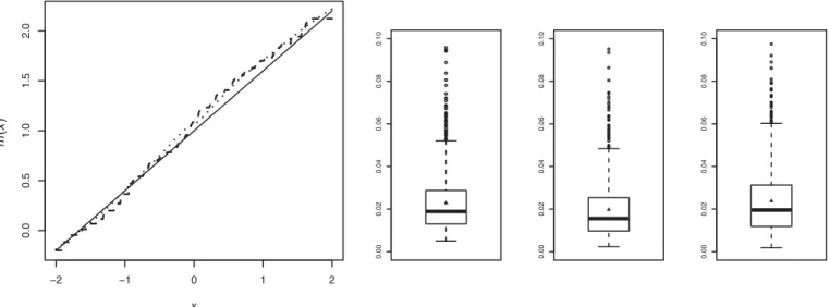
estimate ˆm(x) as is illustrated in Figure 1, where we show

the resulting estimator using ˆF₁,n in the univariate case. To

get a more visually attractive regression curve or surface, one

should smooth the empirical cdf’s ˆF₁,n, . . . ,Fˆd,n. The simple

way to do that is to use a kernel-smoothing method. Letk(·) be

a function, which is a symmetric probability density function

and h≡hn→0 be a bandwidth parameter. Then, a

kernel-smoothing estimator ofFj is given by

˜ Fj,n(x)= 1 n n i=1 K x−Xj,i h ,

where K(x)=_−∞x k(t)dt. The methods of estimating the

marginalsF1, . . . , Fddo not bring out any difference in

asymp-totic behavior of the estimator ˆm(x) as long as they satisfy the

following assumption:

Assumption A. For a given point of interestx ∈Rd_, ˜ Fj,n(xj)=n−1 n i=1 I(Xj,i≤xj)+op(n−1/2), j =1, . . . , d.

Note that the kernel-smoothing estimator ˜Fj,nsatisfies

Assump-tion A ifnh4_{→0. Evidently, this assumption also holds true}

for the rescaled empirical cdf ˆFj,n.

We examined the effect of the methods of estimating the marginal distributions on the regression fit in an extensive sim-ulation study and came to the conclusion that both estimators

( ˆFj,n and ˜Fj,n) show more or less similar performance. Here,

678 Journal of the American Statistical Association, June 2013

Figure 1. Estimated regression functions using ˆF1,n(dashed line) and ˜F1opt,n(dotted line); the black line is the true regression function. Boxplots

of the empirical integrated squared errors of ˆmwith ˆF1,n, ˜F

opt 1,n, and ˜F

cv

1,n, respectively (from left to right).

we present one example to illustrate this. We generate (Y, X₁)

using a Gaussian copula according to DGP S.a described in

Section5. To assess the effect of each method, we consider the

empirical integrated mean squared error (IMSE), the empiri-cal integrated squared bias (IBIAS), and the empiriempiri-cal integrate variance (IVAR), which are given by

IMSE = 1 N N l=1 ISE( ˆm(l))≡ 1 N N l=1 1 I I i=1 ˆ m(l)(xi)−m(xi)2 = 1 I I i=1 m(xi)−m¯ˆ(xi)2 +1 I I i₌1 1 N N l₌1 ( ˆm(l)(xi)−m¯ˆ(xi))2 (7) ≡IBIAS+IVAR,

where {xi,i=1, . . . , I}is a fixed evaluation set, which

cor-responds to a random sample of size I =500 generated from

the distribution of X, ˆm(l)_{(·) is the estimated regression}

func-tion from thelth data sample and ¯ˆm(xi)=N−1N

l=1mˆ( l)_(xi).

Table 1shows the IMSE together with the IBIAS and the IVAR

of ˆm based on N =1000 random samples of size n=100.

We compute ˆmusing ˆF1,n, the rescaled empirical cdf, ˜F1opt,n, the

kernel-smoothing estimate with the mean square optimal band-width, that is,

h_opt(x₁)= 2f1(x1) t k(t)K(t)dt (t2_k(t)dt)2{_f 1(x1)}2 1/3 n−1/3,

and ˜F₁cv_,n, the kernel-smoothing estimate with a bandwidth

cho-sen via the cross-validation (CV) method. Compared with the

Table 1. IBIAS, IVAR, and IMSE (×100) of ˆmdepending on the method of estimatingF1 ˆ F1,n F˜ opt 1,n F˜ cv 1,n

IBIAS IVAR IMSE IBIAS IVAR IMSE IBIAS IVAR IMSE 0.773 1.511 2.282 0.661 1.311 1.971 1.014 1.364 2.377

rescaled empirical cdf, we see in Table 1 that the

kernel-smoothing estimate gives better results if the optimal bandwidth is used. However, when the bandwidth is chosen by the data, its

performance is similar to that of the nonsmooth estimator ˆF1,n.

Figure 1, which shows the boxplots of the empirical integrated squared errors (ISEs), also supports this observation. Based on

that, in all our numerical simulations (see Section5), we use the

rescaled empirical cdf for its simplicity.

As mentioned in the introduction, in this work we adopt a semiparametric approach. For the theoretical analysis, we

as-sume that the true copula densitycbelongs to a certain

para-metric family, which is known. However, in our simulations we consider situations where such a copula family is unknown and should be chosen adaptively using the data. We denote the

cop-ula family to whichcbelongs byC= {c(.;θ), θ∈}, where

is a compact subset ofRp_{. Defineθ}

0to be the true (but

un-known) copula parameter, which lies in the interior ofso that

c(.) coincides withc(.;θ0). We will restrict our interest to an

estimator ˆθnofθ0, which satisfies the following assumption.

Assumption B. ˆ θn−θ0=n−1 n i₌1 ηi+op(n−1/2), (8)

where ηi =η(U0,i,Ui;θ0) is a p-dimensional random vector

such thatEη=0andEηη<∞andUi =(U1,i, . . . , Ud,i).

Many existing estimators forθ0 in the literature satisfy this

assumption. One promising estimator among them is the

(semi-parametric) maximum pseudo-likelihood (PL) estimator ˆθPLn ,

which is defined as the maximizer of

L(θ)= n

i=1

logc( ˆF0,n(Yi),Fn(Xiˆ );θ),

where ˆFn(Xi)=( ˆF1,n(X1,i), . . . ,Fˆd,n(Xd,i)). ˆθ

PL

n was

stud-ied by Genest, Ghoudi, and Rivest (1995), Silvapulle, Kim, and

Silvapulle (2004), Tsukahara (2005), and Kojadinovic and Yan

(2011). Kojadinovic and Yan (2011) compared ˆθPL_n with two

method-of-moment estimators and found that the PL estimator

performs best overall in terms of mean squared error. A sim-ilar conclusion was drawn in Silvapulle, Kim, and Silvapulle

(2004) regarding the comparison of ˆθPL_n with two other

estima-tors based on the maximum likelihood. Assumption B holds for ˆ

θPLn whenever the score function of the density csatisfies the

conditions (A.1)–(A.5) given in Tsukahara (2005). For the PL

estimator, the functionηis given by

η(U₀,U;θ)=J−1(θ)×K(U₀,U;θ), (9) where J(θ)= [0,1]d+1 ∂2 ∂θ∂θlogc(u0,u;θ0) dC(u0,u;θ)

andK(U0,U;θ) is ap-dimensional vector whosekth element

is ∂ ∂θk logc(U0,U;θ)+ d j=0 [0,1]d+1 (I(Uj ≤vj)−vj) × ∂2 ∂θk∂vj logc(v0,v;θ) dC(v0,v;θ).

Remark 1. Tsukahara (2005) stated the conditions under

which the asymptotic normality of ˆθnholds and does not give

explicitly the iid representation in (8). However, to prove the

asymptotic normality, Tsukahara (2005) made use of the

gen-eral theory of Z-estimators, see, for example, sec. A.10 of Bickel

et al. (1993) and chap. 3.3 of van der Vaart and Wellner (1996).

He reduced the problem to the asymptotic normality of a multi-variate rank statistic, the proof of which is a direct consequence of asymptotic linearity and the classical central limit theorem as

given in Ruymgaart (1973, chap. 2).

Before continuing, we need to introduce the following nota-tions:

• ∂jc= _∂u∂c_j forj =0, . . . , d, and∂jcX =∂c_∂uX

j and∂je=

∂e ∂uj

forj =1, . . . , d, wheree(u;θ)=E(Y c(F₀(Y),u;θ)).

• c˙=(_∂θ1∂c, . . . ,_∂θ∂c p) _{, c˙} X =(∂c_∂θ1X, . . . ,∂c_∂θX_p), and e˙= (_∂θ1∂e, . . . ,_∂θ∂e p) _.

Finally, to facilitate the asymptotic analysis, we need the fol-lowing assumptions:

Assumption C. Letg denote either c˙ or ∂jc, j =0, . . . , d

andx∈Rd _{be a given point of interest, which satisfiesF(x)∈}

(0,1)d_.

(C1) (u,θ)→gu0(u,θ)≡g(u0,u;θ) is continuous at (F(x),

θ0) uniformly inu0∈[0,1].

(C2)u0→g(u0,F(x);θ0) is continuous in [0,1].

3. MAIN RESULTS

Now we are ready to present the main results. We will show the asymptotic iid representation of the proposed estimator, which implies that the estimator follows a normal distribution asymptotically.

3.1 Single Covariate Case (d=1)

First, consider the simpler case where there is only one

co-variateX1. In this case,

m(x1)=e(F1(x1);θ0)=E[Y c(F0(Y), F1(x1);θ0)], can be estimated by ˆ m(x1)=eˆ( ˜F1,n(x1); ˆθn)≡n−1 n i=1 Yic( ˆF0,n(Yi),F˜1,n(x1); ˆθn).

The following theorem gives an asymptotic iid representation of this estimator. Its proof is given in the Appendix.

Theorem 1. Assume that ˜F1,n(·), ˆθn, andc(·) satisfy

Assump-tions A, B, and C, respectively. IfEY2 <∞, then we have

√ n( ˆm(x1)−m(x1)) =√1 n n i=1 I(X1,i≤x1)−F1(x1) ∂1e(F1(x1);θ0) − I(Yi ≤y)−F0(y) c(F₀(y), F₁(x₁);θ0)dy +η i e(˙F1(x1);θ0) +op(1).

Theorem 1 implies that√n( ˆm(x₁)−m(x₁)) follows

asymp-totically a normal distribution with mean 0 and varianceσ2₌

var(Ei(θ0)), withEi(θ0) being the term within the bracket in

Theorem 1. By the plug-in principle, a natural estimator ofσ2_is

given by ˆσ2_=n−1n i₌1( ˆEi( ˆθn)−n−1 n i₌1Eˆi( ˆθn))2, where ˆ Ei(θ)=I(X1,i ≤x1)−Fˆ1,n(x1) ∂1e( ˆF1,n(x1); ˆθn) − (I(Yi ≤y)−Fˆ0,n(y))c( ˆF0,n(y),Fˆ1,n(x1);θ)dy +ηˆ_i (θ)ˆ˙e( ˆF1,n(x1); ˆθn), with ηˆi(θ)=η( ˆF0,n(Yi),Fˆ1,n(X1,i);θ), ˆ˙e(u1;θ)=n−1 n i=1 Yic( ˆ˙F0,n(Yi), u1;θ), and∂1e(u1;θ)=n−1 n i=1Yi∂1c( ˆF0,n(Yi),

u₁;θ). The sketch of the proof for the consistency of ˆσ2_{with the}

necessary assumptions is given in the Appendix. Additionally,

we check the consistency empirically in Section5 by

investi-gating the validity of the confidence interval for ˆm(x1) based

on ˆσ2_.

3.2 Multiple Covariate Case (d≥2)

In the general case (d ≥2), the regression function is given

by

m(x)= e(F(x);θ0)

cX(F(x);θ0)

. (10)

Estimating the numerator of m(x) can be done, as in

the single covariate case, by eˆ( ˜Fn(x); ˆθn)≡n−1n

i=1

Yic( ˆF0,n(Yi),Fn(x˜ ); ˆθn), where Fn(x)˜ =( ˜F1,n(x1), . . . ,

˜

Fd,n(xd)). Following the proof of Theorem 1, one can easily

check that under Assumptions A, B, and C, we have ˆ e( ˜Fn(x); ˆθn)−e(F(x);θ0)=n−1 n i=1 Ei(x;θ0)+op(n−1/2), (11)

680 Journal of the American Statistical Association, June 2013

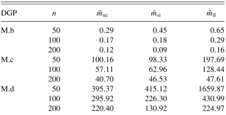
Table 2. IBIAS, IVAR, and IMSE (×1000) of ˆmand ˜m

IBIAS IVAR IMSE IBIAS IVAR IMSE ˆ m 0.172 1.567 1.737 1.178 1.963 3.139 m˜ where Ei(x;θ0)= d j=1 I(Xj,i≤xj)−Fj(xj) ∂je(F(x);θ0) − {I(Yi ≤y)−F0(y)}c(F0(y),F(x);θ0)dy +η i e(F˙ (x);θ0).

From the Equation (6), we consider two estimators for the

de-nominator of (10), which are

˜ cX( ˜Fn(x); ˆθn)= 1 0 c(u₀,Fn(x); ˆ˜ θn)du₀and ˆ cX( ˜Fn(x); ˆθn)=n−1 n i=1 c( ˆF0,n(Yi),Fn(x); ˆ˜ θn).

These two estimators lead to two different estimators form(x),

˜

m(x), and ˆm(x), respectively. However, the difference between

˜

m(x) and ˆm(x) is negligible asymptotically (see the remark

be-low). In our simulation studies, we have found that in many cases

the estimator ˆm(x) is preferable to ˜m(x) in terms of finite sample

performance. To illustrate this remark, we briefly present one small Monte Carlo study designed to compare these two

esti-mators. UsingN =1000 random samples generated from DGP

M.a (d =2) described in Section5, we compute the empirical

IMSE, IBIAS, and IVAR for ˜mand ˆm. FromTable 2, we see

that the latter clearly performs better than the former, both in terms of bias and variance. This observation is also confirmed byFigure 2, which shows the boxplots of the empirical ISEs of the two estimators. From this observation, we only consider

ˆ

m(x) hereafter.

To state the main result about ˆm(x), first note that the

asymp-totic representation of ˆcX( ˜Fn(x); ˆθn) follows by using similar

arguments as in the proof of Theorem 1. In fact, under

Assump-tions A, B, and C, one can easily check that we have ˆ cX( ˜Fn(x); ˆθn)−cX(F(x);θ0)=n−1 n i=1 Di(x;θ0)+op(n−1/2), (12) where Di(x;θ0)= d j=1{I(Xj,i ≤xj)−Fj(xj)}∂jcX(F(x); θ0)+ηi ˙cX(F(x);θ0).

Remark 2. This representation implies that up to

op(n−1/2), ˆcX( ˜Fn(x); ˆθn) is asymptotically equivalent to

1

0 c(u0,Fn(x); ˆ˜ θn)du0. This also means that the difference

be-tween ˜m(x) and ˆm(x) is negligible up to the first-order

approx-imation.

Finally, combining (11) with (12) leads to our main result.

Theorem 2. Assume that every component of ˜Fn satisfies

Assumption A, ˆθn andc(·) satisfy Assumptions B and C,

re-spectively. IfE[Y2]<∞, then we have

√ n( ˆm(x)−m(x))= √1 n n i₌1 1 cX(F(x);θ0) × [Ei(x;θ0)−m(x)Di(x;θ0)]+op(1). As in the univariate case, the asymptotic normality of

√

n( ˆm(x)−m(x)) can be deduced from Theorem 2. The

asymp-totic variance of√n( ˆm(x)−m(x)), which is given by

var 1 cX(F(x);θ0) [E₁(x;θ0)−m(x)D1(x;θ0)] ,

can be estimated using the plug-in method. As a consequence,

one can easily construct pointwise confidence intervals form.

The validity of this approach is investigated in Section5.

4. CONSIDERATION OF MISSPECIFICATION

If the true copula family is known, the proposed estimator performs well as will be shown in the simulation study. However, in practice such information is not available and the copula shape needs to be selected using the data. In any selection procedure,

0.000 0.005 0.010 0.015 0.000 0.005 0.010 0.015

Figure 2. Boxplots of the empirical ISE’s of ˆm(left) and ˜m(right). The triangular dots indicate the average of the ISE.

there is the possibility that the wrong copula family will be selected and using a misspecified copula model for our method

will lead to an inconsistent estimator ofm(x). In this section,

we are interested in the following question: what is the effect (cost) of using a misspecified copula model on the resulting

regression estimator? To answer this question, assume thatC=

{c(.;θ), θ∈}is a parametric family of copula densities under

consideration. In the previous sections, we assumed that the copula family is well-specified, that is, there exists the true

parameterθ0 such thatc(.;θ0) coincides with the true copula

density,c(·), of (Y,X). Under a misspecified model, suchθ0

may not exist. However, even in such a situation, we can define

the pseudo-true parameterθ∗to be the unique minimum within

the setof I(θ)= [0,1]d+1 ln c(u₀,u) c(u₀,u;θ) dC(u0,u).

Here,I(θ) is the classical Kullback–Leibler information

crite-rion expressed in terms of copula densities instead of the tradi-tional densities. Following the lines of the proof for Theorem

2 with θ∗ instead of θ0, we are able to describe the

asymp-totic behavior of ˆm(x) under misspecification in the following

theorem.

Theorem 3. Assume that every component of ˜Fn satisfies

Assumption A and ˆθn andc(·) satisfy Assumptions B and C,

respectively, withθ∗instead ofθ0. IfE[Y2]<∞, then we have

√ n( ˆm(x)−m(x;θ∗))= √1 n n i₌1 1 cX(F(x);θ∗) Ei(F(x);θ∗) − m(x;θ∗)Di(F(x);θ∗) +op(1),

where m(x,θ∗) is the mean regression function under

the assumption that the joint distribution of (Y,X) is

C(F₀(Y),F(X);θ∗). Remark 3. Let ˆ θn=arg min θ n i₌1 logcFˆ₀,n(Yi),Fn(Xi);ˆ θ

be the maximum PL estimator. By the classical maximum

like-lihood theory under misspecification, see White (1982), and

following the proof of Theorem 1 in Tsukahara (2005), we have

verified that ˆθnsatisfies Assumption B with ηas given by (9)

but withθ∗instead ofθ0.

Clearly, this theorem reduces to Theorem 2 when the cop-ula family is well specified. Additionally, the result implies that

under the misspecification, the estimator ˆm(x) is still

asymp-totically normal but is biased. More specifically, a misspecified

copula brings out a bias in the estimation of m(x), which is

(asymptotically) nothing but the difference betweenm(x), the

true regression function, andm(x;θ∗) its best approximation

(in terms of likelihood) among the regression function family

{m(x;θ)≡E(Y c(F0(Y),F(x);θ))/cX(F(x);θ), θ∈}. As a

result, it is important to choose a rich and flexible copula family

to make the differencem(x)−m(x;θ∗) small. More discussion

about this will be given in the next section.

5. SIMULATIONS

The objective of this section is first to check whether the

asymptotic theory for ˆm(x) works both when the copula is well

specified (Theorem 2) and when the copula is misspecified (The-orem 3). The second objective is to compare our semiparametric estimator with some competitors both when the true copula fam-ily is known and when the copula famfam-ily and its parameters are adaptively selected using the data. To this end, we consider the following data generating procedures (DGPs):

• DGP S.a(F0(Y), F1(X1))∼Gaussian copula with

param-eterρ1;Y ∼N(μY, σY2).

(i) The resulting regression function is m(x1)=μY+

σYρ1−1(F1(x1)),where is the cdf of a standard

normal distribution.

(ii) X1is generated fromN(μX1, σ

2 X1).

• DGP S.b(F₀(Y), F₁(X₁))∼FGM copula with parameter

θ;Y ∼N(μY, σY2).

(i) The resulting regression function is m(x₁)=μY−

θ

√_πσY+2√θ_πσYF1(x1).

(ii) X₁ is generated from the cdf FX1(x1)=1−

exp(−exp(x1)).

• DGP S.c (F₀(Y), F₁(X₁))∼Student’st copula with

pa-rametersρanddf;Y ∼N(μY, σY2).

(i) The resulting regression function is

m(x1)=μY+E

σY−1(df(ρa

+Tdf(1−ρ2₎₍₁+_a2_/df)/(df+_1))),

wherea =−_df1(FX1(x1)).df is the cdf of a

univari-ate Student’st-distribution with degrees of freedomdf

andTis a univariate Student’strandom variable with

degrees of freedomdf+1.

(ii) X1is generated fromN(μX1, σ

2 X1) .

• DGP S.d(F₀(Y), F₁(X₁))∼Clayton copula with

parame-tersδ;Y ∼N(μY, σY2).

(i) The resulting regression function is

m(x1)=μY+E σY−1(T−1/δ) , where T ∼fT(t)=(1/δ+1)(1+ξ)(1/δ+1)/(t+ ξ)(1/δ+2)_{fort >1 andξ =F} X1(x1)−δ−1.

(ii) X1is generated fromN(μX1, σ

2 X1).

• DGP M.a(F₀(Y), F₁(X₁), . . . , Fd(Xd))∼Gaussian

cop-ula with correlation matrix=[_ρ1 ρ

X], whereρis a

d-dimensional vector;Y ∼U(0,1).

(i) The resulting regression function is

m(x)= ⎛ ⎝d j₌1 aj 2−ρa −1_(F j(xj)) ⎞ ⎠, wherea=(a1, . . . , ad)≡−X1ρ.

(ii) Xj is generated fromN(μXj, σ

2

Xj), j=1, . . . , d.

682 Journal of the American Statistical Association, June 2013

Table 3. Parameters of the copula and of the marginal distributions for each DGP

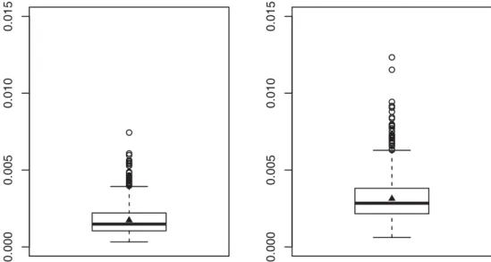
DGP Copula parameter Marginal parameter m

S.a ρ1=0.6 μX1=0, μY =1 1+0.6x1 σX1=σY =1 S.b θ=0.8 μY =0, σY =1 0.8/ √ π−1.6/√πexp(−exp(x1)) S.c ρ=0.6,df =3,5,100 μX1=0, μY =1 No simple form σX1=σY =1 S.d δ=1 μX1=0, μY =1 No simple form σX1=σY =1 M.a (d=2) = ⎛ ⎝₋01.5 −01.5 −00.9.4 0.9 −0.4 1 ⎞ ⎠ μX1=μX2=0 (−0.154x1+0.771x2) σX1=σX2=1 M.a (d=3) = ⎛ ⎜ ⎜ ⎝ 1 0.23 0.90 0.67 0.23 1 0.51 0.26 0.90 0.51 1 0.49 0.67 0.26 0.49 1 ⎞ ⎟ ⎟ ⎠ μX1=μX2=μX3=0, (−0.3x1+0.9x2+0.3x3) σX1=σX2=σX3=1 The parameters of the copula and of the marginal distributions

that we use for each DGP are given inTable 3. All computations

are done with R (R Development Core Team2010).

5.1 Verifying the Asymptotic Results

To verify the established asymptotic results, we draw

Quantile-Quantile (Q-Q) plots of ˆm(x) and calculate empirical

coverage probabilities (ECPs) of the (1−α)-confidence

inter-vals of m(x) calculated according to Theorem 2. ECP means

the proportion of confidence intervals that contain the true value

of the regression functionm(x). By seeing whether the ECPs

are close to the nominal level (1−α), we can check that the

proposed estimator ˆm(x) is asymptotically normal. Also, we

can validate the asymptotic iid representation for ˆm(x) and the

appropriateness of the proposed variance estimator of ˆm(x). We

calculate the estimator ˆm(x) fromN =1000 random samples of

sizen=50,100,200,and 400. This is done for different values

of significance levelα and points of interestx. Only selected

and representative results are shown to save space.

5.1.1 When the Copula is Well Specified. Table 4presents

the ECP of the 95% confidence intervals for m(x) with data

generated from DGP S.a, DGP S.b, and DGP M.a (d=2). We

calculate the ECP, when x is an interior point (x=μX, the

mean of the distribution of X) and a boundary point (a point

that satisfiesP(X−μX>x−μX)=0.1, where · is

the Euclidean norm). As seen inTable 4, even for a small sample

size, the ECPs are generally quite close to their nominal confi-dence level. This demonstrates the validity of our iid represen-tation and the consistency of our asymptotic variance estimator.

Figure 3, which shows the Q-Q plots for our estimator with DGP

S.b whenn=50, also confirms this finding. These plots clearly

indicate the accuracy of the normal approximation to the

asymp-totic distribution of ˆm(x). To estimate the copula parameter, we

make use of the R packagecopula(see Yan2007).

5.1.2 When the Copula is Misspecified. To verify the asymptotic behavior of our estimator under misspecification,

we generate data from Student’stcopula and Clayton copula

according to DGP S.c and DGP S.d, respectively, but in our estimation procedure we use a Gaussian copula. To see how the degree of misspecification influences our estimator, we vary the

degrees of freedom (df) of the Student’s copula in{3,5,100}.

Since the difference between the best approximationm(x₁, ρ∗)

and the true valuem(x₁) depends on the distance between the

given copula familyC= {c(.;θ), θ∈}and the true copula

c(·), we expect to see the estimator ˆm(x1) concentrating more

aroundm(x1) as thedf of the truet-copula increases based on

our established theory. The “pseudo”-true regression function

ism(x1, ρ∗)=1+ρ∗x1withρ∗=0.583,0.590,0.596 for the

t-copulas (df=3,5,100), respectively, andρ∗=0.503 for the Clayton copula.

Figure 4shows the boxplots of the estimators ˆm(x1) obtained from 1000 random samples of size 200. As stated in Theorem 3, we see that the observed values are symmetrically distributed

around the pseudo-true parameter m(x₁, ρ∗) instead of true

parameter ˆm(x₁). The difference between these two quantities

corresponds exactly to the asymptotic bias. This bias decreases as the “distance” between the true and the used copula decreases.

In case of the t-copula, our estimator becomes consistent as

thedfincreases. Clearly, the selection of an appropriate copula

family is important for guaranteeing good performance of our methodology considering the case of the Clayton copula.

Table 4. Coverage probabilities of the proposed confidence interval form(x),α=0.05

DGP x n=50 n=100 n=200 n=400 Interior S.a 0.00 0.943 0.938 0.939 0.953 S.b −0.58 0.953 0.952 0.951 0.949 M.a (d=2) (0.00,0.00) 0.946 0.943 0.937 0.943 Boundary S.a −1.64 0.907 0.933 0.956 0.950 S.b −2.49 0.968 0.957 0.962 0.955 M.a (d=2) (1.53,1.53) 0.946 0.945 0.946 0.962

−3 −2 −1 0 1 2 3 −0.4 −0.2 0.0 0.2 0.4 Theoretical Quantiles m^

(

)

(

)

Figure 3. Q-Q plots of ˆm(x) at an interior point (left) and at a boundary point (right).n=50, DGP S.b.

5.2 Robustness and Comparison With Other Methods

In this section, we compare our semiparametric estimator both with semiparametric and nonparametric competitors. We consider four estimators for comparison.

• mˆ_tc: our estimator when the true copula family is used.

• mˆ_uc: our estimator when the copula density family is

adap-tively selected using the data (see the explanation below).

• mˆll: local linear estimator with the bandwidth selected by

CV using the R packagenp(see Hayfield and Racine2008).

• mˆsi: single index regression estimator based on a two-stage

estimation method; the single index coefficients are first

estimated by the R packagedr using the slice inverse

re-gression method (see Li1991) and then the link function

is estimated in the same way as for ˆmll.

When no information is available about the true copula den-sity, we should choose an appropriate copula family for our

estimator ˆm_uc. This step may be difficult especially when the

number of covariates is large. The reason is that the set of

high-dimensional copulas available in the literature is limited to very special and restrictive copula families such as elliptical copu-las and Archimedean copucopu-las. For this reason, the strategy that we advocate and adopt here is to make use of the recent avail-able work about the simplified pair-copula decomposition. The main idea is to decompose a multivariate copula to a cascade of bivariate copulas so that we can take advantage of the rela-tive simplicity of bivariate copula selection and estimation. To be more specific, we briefly describe such an approach for the

case of a three-variate vectorX =(X1, X2, X3). By applying

Sklar’s theorem recursively, one can write, for example,

c(F0(y), F1(x1), F2(x2), F3(x3))

= cX(F1(x1), F2(x2), F3(x3))c01(F0(y), F1(x1))

×c02|1(F0|1(y|x1), F2|1(x2|x1)|x1)

×c03|12(F0|12(y|x1, x2), F3|12(x3|x1, x2)|x1, x2), (13)

wherec₀₁,c_02|1andc_03|12are the copula densities associated with

the distributions of (Y, X₁), (Y, X₂)|X₁, and (Y, X₃)|(X₁, X₂),

0.2 0.3 0.4 0.5 0.6 0.7 0. 8 Clayton 0.2 0.3 0.4 0.5 0.6 0.7 0. 8 t(df=3) 0.2 0.3 0.4 0.5 0.6 0.7 0. 8 t(df=5) 0.2 0.3 0.4 0.5 0.6 0.7 0. 8 t(df=100)

Figure 4. Boxplots of ˆm(x1) atx1=F1−1(0.2)= −0.8416 for different degree of freedom. The horizontal solid line representsm(x1, ρ∗) and

the dotted line representsm(x1).

684 Journal of the American Statistical Association, June 2013

respectively. Similarly,cXcan be, for example, decomposed as

cX(F1(x1), F2(x2), F3(x3))

=c12(F1(x1), F2(x2))c23(F2(x2), F3(x3))c13|2(F1|2(x1|x2),

×F3|2(x3|x2)|x2).

If we assume that all the conditional copulas depend on the conditioning variables only through the conditional

distributions, for example, c_02|1(F_0|1(y|x₁), F_2|1(x₂|x₁)|x₁)=

c_02|1(F_0|1(y|x₁), F_2|1(x₂|x₁)), then it leads to the so-called

sim-plified pair-copula decomposition. Because any bivariate copula density can be used as a building block for this decomposition, the simplified pair-copula decomposition provides high flexibil-ity and the abilflexibil-ity to cover a wide range of complex

dependen-cies. Hobæk Haff, Aas, and Frigessi (2010) and Stoeber, Joe,

and Czado (2012) discussed the conditions under which such a

simplification is possible and found that this is not a severe re-striction in many situations. For more about this decomposition,

see the recent book by Kurowicka and Joe (2010).

In our simulation, for our estimator ˆmuc, we choose one

decomposition (R-vine structure) for the data and then choose the pair-copulas independently among 10 candidate copulas:

two are elliptical (Gaussian and Student’s t) and eight are

Archimedean (Clayton, Gumbel, Frank, Joe, Clayton–Gumbel, Joe–Gumbel, Joe–Clayton, and Joe–Frank) using the R package VineCopula; see Dißmann et al. (2011). As a selection criterion for bivariate copula, we use the Akaike information criterion (AIC).

Remark 4. As noted by the referees, instead of using the classical AIC, which lacks theoretical justification in the context of pseudo-maximum likelihood, it is possible to use the copula

information criterion (CIC); see Grønneberg and Hjort (2011)

and Grønneberg (2011). However, the CIC does not exist for

some popular copula families such as Gumbel and Joe copulas and is complicated to compute even when it exists. Compared with the CIC, the AIC is easy to compute and has been shown to perform well for copula selection in R-vine framework; see

Brechmann (2010, chap. 5).

5.2.1 When the Simplified Pair-Copula Assumption Holds. To generate data that satisfy our copula assumptions, we

con-sider DGP M.a (d =2) and M.a (d =3). As a reference case,

we consider the nonlinear least-square estimator ˆmls with the

true link function. We use the R packagenlrwrto calculate ˆmls.

For details, we refer to Ritz and Streibig (2008).Table 5shows

the IMSE of each estimator. As expected, the least-square

esti-mator ˆmlsgives the best performance. The difference in IMSE

Table 5. 100×IMSE for ˆmls(least square), ˆmtc(true copula), ˆmuc

(unknown copula), and ˆmll(local linear)

DGP n mlsˆ mtcˆ mucˆ msiˆ mllˆ M.a (d=2) 50 0.067 0.177 0.205 0.332 0.637 100 0.029 0.079 0.097 0.196 0.197 200 0.015 0.038 0.047 0.059 0.098 M.a (d=3) 50 0.030 0.195 0.229 0.404 0.547 100 0.014 0.092 0.107 0.283 0.159 200 0.007 0.045 0.052 0.048 0.076

Table 6. Specification of DGP M.b, DGP M.c, and DGP M.d.is the cdf of the standard Cauchy distribution

DGP m(X) σ

M.b (−0.3X1+0.9X2+0.3X3) 0.1

M.c √|2X1−X2+0.5| +(−0.5X3+1)(0.1X3

4) 2

M.d ((−2X1+X2−4X3+3X4+X5+2X6)/√35)3 _0.5

between ˆm_lsand our copula estimators decreases as the sample

size increases. Since additional variability comes into the esti-mation from the selection of copula family for each bivariate

copula, ˆmuchas larger IMSE than ˆmtcbut the difference is

rel-atively moderate. The reason for the modest difference is that the Gaussian copula admits R-vine decompositions with

Gaus-sian pair-copulas (see Hobæk Haff, Aas, and Frigessi2010) and

the AIC works reasonably well. We observe that the estimator ˆ

mucdoes better than the local linear estimator on the whole and

especially at boundary regions (the details are not shown here). The same remarks remain valid in three-covariate case. In this

case, it is important to note that the difference between ˆmtcand

ˆ

m_ucbecomes bigger than in two-covariate case especially when

the sample size is small. This is because the number of bivariate copula to be selected and estimated by the data in the decompo-sition increases with the number of the covariates (six instead of

three in our case). However, whend =3, ˆm_ucstill remains

sig-nificantly better than the local linear estimator, which is known to suffer from the curse of dimensionality. Finally, it is notable

that our estimator ˆmucis even better than the single index

esti-mator ˆmsioverall. The reason for it may be that the uncertainty

stemming from the copula choice is relatively smaller than that coming from the estimation of the single index coefficients when the dimension of the covariates is relatively small.

5.2.2 When the Simplified Pair-Copula Assumption Does not Hold. In this section, we investigate how our estimator performs when the true copula does not belong to the class of R-vines under consideration. For such purpose, we generate the data from DGP M.b, DGP M.c, and DGP M.d, which are

based on the regression model Y =m(X)+σ , where X is

multivariate normal with mean 0 and cov(Xi, Xj)=0.5|i−j|

and∼N(0,1) independent ofX. Specification of each DGP

is given inTable 6.

In these cases, to our knowledge, the true copula densities cannot fit into any simplified pair-copula decomposition with

Table 7. 100×IMSE for ˆmuc(unknown copula), ˆmsi(single index), and ˆmll(local linear)

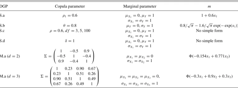
DGP n mˆuc mˆsi mˆll M.b 50 0.29 0.45 0.65 100 0.17 0.18 0.29 200 0.12 0.09 0.16 M.c 50 100.16 98.33 197.69 100 57.11 62.96 128.44 200 40.70 46.53 47.61 M.d 50 395.37 415.12 1659.87 100 295.92 226.30 430.99 200 220.40 130.92 224.97

5 10 15 20 −1.5 −1.0 −0.5 0.0 0.5 1.0 1.5 wind (AD) resid u al 5 10 15 20 −1.5 −1.0 −0.5 0.0 0.5 1.0 1.5 wind (SI) resid u al 5 10 15 20 −1.5 −1.0 −0.5 0.0 0.5 1.0 1.5 wind (CO) resid u al

Figure 5. Residual plots for (AD), (SI), and (CO).

the bivariate copulas in our candidate list. Consequently, the

performance of ˆmucis affected by the misspecification caused

by assuming the pair-copula decomposition and arising in the

bivariate copula selection.Table 7shows that on the whole our

estimator ˆmuc has better performance than the nonparametric

estimator ˆmllespecially when the sample size is small and the

number of covariates is large. In the cases of DGP M.b and M.d, where the true model is a single-index model, our

esti-mator ˆmucperforms similarly to the estimator ˆmsibut with ˆmsi

having a slight advantage. This is natural because the estimator ˆ

m_si directly exploits the information about the true regression

structure. However, under DGP M.c where the single index

as-sumption is not correct, our estimator ˆm_ucseems to work better

than the other estimators ˆm_siand ˆm_ll.

6. REAL DATA ANALYSIS

To illustrate our method, we analyze data from air pollution studies. The data consist of measurements of daily ozone

con-centration (Y =log(ozone)), solar radiation (X1=rad), daily

maximum temperature (X2 =temp), and wind speed (X3=

wind) onn=111 days from May to September 1973 in New

York. To estimatem(X1, X2, X3)=E(Y|X1, X2, X3), we

con-sider the following:

(LL) Local linear estimator with the bandwidth selected by CV.

(LS) Least-square estimator ˆβ0+βˆ1rad+βˆ2temp+βˆ3wind+

ˆ

β4wind2.

(AD) Additive model estimator ˆg1(rad)+gˆ2(temp)+gˆ3(wind).

(SI) Single index model estimator gˆ( ˆβ1rad+βˆ2temp+

ˆ

β3wind).

Table 8. Cross-validation error of each estimator for ozone data (LS) (AD) (SI) (CO) (LL) CV1 0.3183 0.2917 0.4465 0.2768 0.2815

CV2 0.2174 0.2203 0.3446 0.2065 0.1701

(CO) Our copula-based estimator with the copula selected by the data using pair-copula decomposition.

Model (LS) was considered by Crawley (2005), who found

that the quadratic model fitted the data well. (AD), (SI), and (CO) are semiparametric models. We use a smoothing spline to

fit the AD using R packagegamand a local linear estimator to

fit the SI. Finally, as an evaluation measure of each estimator, we compute the following two versions of CV error:

CV1( ˆm)=median1≤i_≤n|Yi−mˆ₋i(Xi)| and

CV2( ˆm)=

n

i₌1

(Yi−mˆ−i(Xi))2, (14)

where ˆm₋i(Xi) is the estimate of m(Xi) from the dataset

{(Yj,Xj);j =i, j =1, . . . , n}. CV1is a robustified version of

the standard CV error CV2.

Table 8 suggests that all the estimators except (SI) show more or less similar performances with our method having a slight advantage. Clearly, the single index structure is not ap-propriate for this data and the additive structure seems to be more adequate. In terms of the CV criteria, our estimator shows

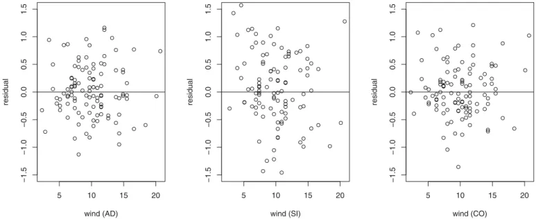
very good performance. The residual plots betweenX3,i(wind)

andYi−mˆ−i(Xi) for (AD), (SI), and (CO), seeFigure 5, also

support these remarks. We observe that the residuals from (SI)

show a decreasing trend asX3(wind) increases while the

resid-uals from (AD) and (CO) show a random pattern. This example clearly shows the flexibility of our estimator and its ability to adapt to the underlying regression structure of the data.

7. CONCLUSION AND FUTURE WORKS

We proposed a new semiparametric estimator of a regression function based on copulas. The estimator is obtained by model-ing the joint distribution of the response and its covariates via a parametric copula family and the marginals via nonparametric methods. This method is flexible, easy to implement and seems to be less influenced by the curse of dimensionality. However, this advantage is attained at the price of a model risk in the

686 Journal of the American Statistical Association, June 2013 copula modeling. Here, we empirically checked that such a

model risk was small but some theoretical analysis about the ad-ditional risk stemming from the model selection step is needed. Additionally, since copula has some advantages in modeling tail dependence, it would be interesting to see whether our cop-ula regression framework benefits from those advantages in the estimation when the data have a specific tail dependence.

APPENDIX: TECHNICAL DETAILS

Lemma 1. Assume thatcsatisfies Assumption C. If (i)E|Y|<∞, (ii) ˜F1,n(x1)−F1(x1)=Op(n−1/2), and (iii) ˆθn−θ0=Op(n−1/2), then

we have ˆ m(x1)=n−1 n i=1 Yic(F0(Yi), F1(x1);θ0)+n−1 n i=1 Yi( ˆF0,n(Yi) −F0(Yi))∂0c(F0(Yi), F1(x1);θ0)+( ˜F1,n(x1) −F1(x1))∂1e(F1(x1);θ0)+( ˆθn−θ0)e˙(F1(x1);θ0) +op(n−1/2).

Proof. Using the first-order Taylor expansion, we have ˆ m(x1)=n−1 n i=1 Yic(F0(Yi), F1(x1);θ0)+V1,n+V2,n+V3,n, (A.1) where V1,n=n−1 n i=1 Yi( ˆF0,n(Yi)−F0(Yi))∂0c( ˜U0,i,U1˜ ,i; ˜θi,n), V2,n=n−1 n i=1 Yi( ˜F1,n(x1)−F1(x1))∂1c( ˜U0,i,U˜1,i; ˜θi,n), V3,n=n−1 n i=1 Yi( ˆθn−θ0)˙c( ˜U0,i,U1˜ ,i; ˜θi,n),

with ˜U0,i=F0(Yi)+ti,n( ˆF0,n(Yi)−F0(Yi)), ˜U1,i=F1(x1)+ti,n( ˜F1,n

(x1)−F1(x1)), and ˜θi,n=θ0+ti,n( ˆθn−θ0) for some random quantity ti,n∈[0,1]. By adding and subtracting ∂0c(F0(Yi), F1(x1);θ0) in the

sum, decompose further the termV1,nas

V1,n=n−1 n i=1 Yi( ˆF0,n(Yi)−F0(Yi))∂0c(F0(Yi), F1(x1);θ0)+Rn, where Rn=n−1 n i=1 Yi( ˆF0,n(Yi)−F0(Yi))[∂0c( ˜U0,i,U1˜ ,i; ˜θi,n) −∂0c(F0(Yi), F1(x1);θ0)].

To show Rn=op(n−1/2), first note that n−1

n

i=1|Yi| =Op(1) and

supy|F0ˆ,n(y)−F0(y)| =Op(n−1/2) by Donsker’s Theorem. Moreover,

by Assumption C and the continuous mapping theorem, we have max 1≤i≤n∂0c( ˜U0,i, ˜ U1,i; ˜θi,n)−∂0c( ˜U0,i, F1(x1);θ0)=op(1); sup |u˜0−u0|<n |∂0c( ˜u0, F1(x1);θ0)−∂0c(u0, F1(x1);θ0)| =op(1) whenevern=op(1).

Consequently, by the triangle inequality, we have max

1≤i≤n∂0c( ˜U0,i,

˜

U1,i; ˜θi,n)−∂0c(F0(Yi), F1(x1);θ0)=op(1),

which leads toRn=op(n−1/2). Thus, we know that

V1,n=n−1 n i=1 Yi( ˆF0,n(Yi)−F0(Yi))∂0c(F0(Yi), F1(x1);θ0)+op(n−1/2). (A.2) Now, we turn to the second termV2,n. Following the same arguments

as forV1,nwith Assumption (ii), we have

V2,n=( ˜F1,n(x1)−F1(x1))n−1 n i=1 Yi∂1c(F0(Yi), F1(x1);θ0)+op(n−1/2) =( ˜F1,n(x1)−F1(x1))∂1e(F1(x1);θ0)+op(n−1/2). (A.3)

In the last equality, we use the fact that n−1n

i=1Yi∂1c(F0(Yi),

F1(x1);θ0) converges in probability toE(Y ∂1c(F0(Y), F1(x1);θ0))= ∂1e(F1(x1);θ0).Similarly, using Assumption (iii), the last term V3,n

can be expressed as V3,n=( ˆθn−θ0)n−1 n i=1 Yi˙c(F0(Yi), F1(x1);θ0)+op(n−1/2) =( ˆθn−θ0)e˙(F1(x1);θ0)+op(n−1/2). (A.4)

Recollecting the elements (A.2), (A.3), (A.4), and (A.1) gives the claimed result.

Proof of Theorem 1

Put V˜1,n=n−1

n

i=1Yi( ˆF0,n(Yi)−F0(Yi))∂0c(F0(Yi), F1(x1);θ0).

This is aV-statistic with the kernel

h(Yi, Yj)= 1 2 Yi(I(Yj≤Yi)−F0(Yi))∂0c(F0(Yi), F1(x1);θ0) +Yj(I(Yi≤Yj)−F0(Yj))∂0c(F0(Yj), F1(x1);θ0) .

By Assumption C and (i), we haveE[h2_(Y

i, Yj)]<∞. Therefore, using

Lemma 5.7.3 and Theorem 5.3.2 in Serfling (1980) and the fact that

Eh(Yi, Yj)=0, we get that ˜ V1,n=n−1 n i=1 λ(Yi, F1(x1);θ0)+op(n−1/2), (A.5) where λ(u0, u1;θ)= y{I(u0≤y)−F0(y)}∂0c(F0(y), u1;θ)f0(y)dy.

Using integration by part and the fact thatE|Y|<∞, it is easy to check that λ(u0, u1;θ)= yc(F0(y), u1;θ0)f0(y)dy−u0c(F0(u0), u1;θ0) − (I(u0≤y)−F0(y))c(F0(y), u1;θ0)dy.

This result together with Lemma 1, Assumptions A, and B concludes the proof.

Sketch of the Proof for the Consistency of ˆσ2

Here, we sketch the proof for the single parameter (p=1) and single covariate (d=1) case . The proof for the general case can be done in a similar way. To prove the consistency, we mainly need to prove that

n−1 n i=1 ˆ E2 i( ˆθn)=n−1 n i=1 ˆ E2 i(θ0)+op(1) (A.6) =n−1 n i=1 Ei2(θ0)+op(1). (A.7)