Statistical Methods for the Analysis of Mass Spectrometry-based Proteomics Data

STATISTICAL METHODS FOR THE ANALYSIS OF MASS

SPECTROMETRY-BASED PROTEOMICS DATA

A Dissertation

by

XUAN WANG

Submitted to the Office of Graduate Studies of Texas A&M University

in partial fulfillment of the requirements for the degree of

DOCTOR OF PHILOSOPHY

May 2012

STATISTICAL METHODS FOR THE ANALYSIS OF MASS

SPECTROMETRY-BASED PROTEOMICS DATA

A Dissertation

by

XUAN WANG

Submitted to the Office of Graduate Studies of Texas A&M University

in partial fulfillment of the requirements for the degree of

DOCTOR OF PHILOSOPHY

Approved by:

Chair of Committee, Alan R. Dabney

Committee Members, Michael T. Longnecker Huiyan Sang

Joseph Sturino Head of Department, Simon J. Sheather

May 2012

ABSTRACT

Statistical Methods for the Analysis of Mass Spectrometry-based Proteomics Data. (May 2012)

Xuan Wang, B.S., University of Science and Technology of China, Anhui, China; M.S., Texas A&M University

Chair of Advisory Committee: Dr. Alan R. Dabney

Proteomics serves an important role at the systems-level in understanding of biological functioning. Mass spectrometry proteomics has become the tool of choice for identifying and quantifying the proteome of an organism. In the most widely used bottom-up approach to MS-based high-throughput quantitative proteomics, complex mixtures of proteins are first subjected to enzymatic cleavage, the resulting peptide products are separated based on chemical or physical properties and then analyzed using a mass spectrometer. The three fundamental challenges in the analysis of bottom-up MS-based proteomics are as follows: (i) Identifying the proteins that are present in a sample, (ii) Aligning different samples on elution (retention) time, mass, peak area (intensity) and etc, (iii) Quantifying the abundance levels of the identified proteins after alignment. Each of these challenges requires knowledge of the biological and technological context that give rise to the observed data, as well as the application of sound statistical principles for estimation and inference. In this dissertation, we present a set of statistical methods in bottom-up proteomics towards protein identification, alignment and quantification.

We describe a fully Bayesian hierarchical modeling approach to peptide and pro-tein identification on the basis of MS/MS fragmentation patterns in a unified frame-work. Our major contribution is to allow for dependence among the list of top candidate PSMs, which we accomplish with a Bayesian multiple component mixture

iv model incorporating decoy search results and joint estimation of the accuracy of a list of peptide identifications for each MS/MS fragmentation spectrum. We also propose an objective criteria for the evaluation of the False Discovery Rate (FDR) associated with a list of identifications at both peptide level, which results in more accurate FDR estimates than existing methods like PeptideProphet.

Several alignment algorithms have been developed using different warping func-tions. However, all the existing alignment approaches suffer from a useful metric for scoring an alignment between two data sets and hence lack a quantitative score for how good an alignment is. Our alignment approach uses “Anchor points” found to align all the individual scan in the target sample and provides a framework to quantitify the alignment, that is, assigning a p-value to a set of aligned LC-MS runs to assess the correctness of alignment. After alignment using our algorithm, the p-values from Wilcoxon signed-rank test on elution (retention) time, M/Z, peak area successfully turn into non-significant values.

Quantitative mass spectrometry-based proteomics involves statistical inference on protein abundance, based on the intensities of each protein’s associated spec-tral peaks. However, typical mass spectrometry-based proteomics data sets have substantial proportions of missing observations, due at least in part to censoring of low intensities. This complicates intensity-based differential expression analysis. We outline a statistical method for protein differential expression, based on a simple Binomial likelihood. By modeling peak intensities as binary, in terms of “presence / absence”, we enable the selection of proteins not typically amendable to quantitative analysis; e.g., “one-state” proteins that are present in one condition but absent in another. In addition, we present an analysis protocol that combines quantitative and presence / absence analysis of a given data set in a principled way, resulting in a single list of selected proteins with a single associated FDR.

vi ACKNOWLEDGMENTS

I would like to express my sincerest appreciation to my advisor, Dr. Alan R. Dabney, for his direction, suggestion, encouragement, patience and continuous sup-port toward my professional development. He guided me to think about statistical research problems, how to do research and how to write a paper step by step.

I am very grateful to all my committee members, Dr. Michael Longnecker, Dr. Huiyan Sang, Dr. Joseph Sturino, for their guidance and support throughout the course of this research.

Thanks also go to my friends and colleagues and the department faculties and staff for making my time at Texas A&M University a great experience.

Finally, I feel lucky to have my husband, my son and my parents be my side, thank you for your unconditional love.

This research is supported by the. This work was sponsored by a subcontract from PNNL and by the NIH R25-CA-90301 training grant at TAMU. Additional support was provided by KAUST-IAMCS Innovation grant, by NIH grant DK070146 and by the National Institute of Allergy and Infectious Diseases (NIH/DHHS through interagency agreement Y1-AI-4894-01).

NOMENCLATURE

AMT Accurate mass and time

ANOVA Analysis of variance

CDF Cumulative density function

FDR False discovery rate

GEV Generalized extreme value

LC-MS Liquid chromatographyCMass spectrometry

M/Z Mass over charge ratio

NET Normalized elution time

NMC Number of missed cleavage sites

NTE Number of tryptic ends

PEP Posterior error probability

PM Potential matches

PMF Probability mass function

PNNL Pacific northwest national laboratory

PSM Peptide spectrum match

RBF Radial basis function

RT Retention Time

viii TABLE OF CONTENTS Page ABSTRACT . . . iii DEDICATION . . . v ACKNOWLEDGMENTS . . . vi NOMENCLATURE . . . vii

TABLE OF CONTENTS . . . viii

LIST OF TABLES . . . xi

LIST OF FIGURES . . . xii

1 INTRODUCTION . . . 1 1.1 General Background . . . 1 1.2 LC-MS Proteomics . . . 2 1.3 Peptide/Protein Identification . . . 6 1.4 Alignment . . . 9 1.5 Protein Quantitation . . . 14

2 A BAYESIAN HIERARCHICAL MODEL FOR PEPTIDE / PROTEIN IDENTIFICATION BY LC-MS/MS. . . 16

2.1 Introduction . . . 16

2.2 Methods . . . 18

2.2.1 Experiments . . . 18

2.2.2 Peptide and Protein Identification by Database Search . . . . 18

2.2.3 Model . . . 22

2.2.4 Bayesian Implementation and Bayesian False Discovery Rate . 34 2.3 Results . . . 35

2.4 Discussion . . . 39

3 A STATISTICAL APPROACH TO THE ALIGNMENT OF LC-MS/MS SAMPLES . . . 40

Page

3.1 Introduction . . . 40

3.1.1 Background . . . 40

3.1.2 Existing Alignment Methods . . . 40

3.2 Methods . . . 42

3.2.1 Anchor Points . . . 42

3.2.2 Alignment Algorithm . . . 43

3.3 Real Data Example . . . 45

3.3.1 Visualization of Alignment . . . 45

3.3.2 Global P-value for Alignment Performance . . . 49

3.3.3 Local P-values for Alignment Performance . . . 51

3.4 Discussion . . . 54

4 A HYBRID APPROACH TO PROTEIN DIFFERENTIAL EXPRESSION IN MASS SPECTROMETRY-BASED PROTEOMICS . . . 55

4.1 Introduction . . . 55

4.2 Methods . . . 57

4.2.1 Data . . . 57

4.2.2 Logistic Model for Protein Presence / Absence . . . 58

4.2.3 Peptide-level Exact Test . . . 60

4.2.4 Protein-level Bootstrap Test . . . 61

4.2.5 False Discovery Rate (FDR) Estimation . . . 62

4.2.6 Hybrid Analysis Incorporating Both Presence / Absence and Intensity Measurements . . . 67

4.3 Results . . . 68

4.3.1 Peptide-level Simulation Result . . . 68

4.3.2 Protein-level Simulation Result . . . 70

4.3.3 Mixed Single-peptide Protein and Multi-peptide Protein Sim-ulation Result . . . 72

4.3.4 Hybrid Approach Simulation Result . . . 74

4.3.5 Diabetes Data . . . 74

4.4 Discussion . . . 76

x

Page

REFERENCES

. . . .

. . . .

. . .

.

. . . .

.

. . . .

LIST OF TABLES

TABLE Page

3.1 A sample record of SEQUEST output. . . 42 4.1 Peptide-level error rates and power with p1 = 0.2,0.3,0.4,0.5 and pd =

0.0,0.1, . . . ,0.7. . . 70 4.2 Protein-level error rates and power with p1 = 0.2,0.3,0.4,0.5 and pd =

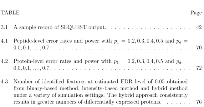
0.0,0.1, . . . ,0.7. . . 72 4.3 Number of identified features at estimated FDR level of 0.05 obtained

from binary-based method, intensity-based method and hybrid method under a variety of simulation settings. The hybrid approach consistently results in greater numbers of differentially expressed proteins. . . 76

xii LIST OF FIGURES

FIGURE Page

1.1 Mass spectrometry. The mass spectrometer consists of an ion source, responsible for ionizing peptides, the mass analyzer and the detector, responsible for recording m/z values and intensities, respectively, for each ion species. Each MS scan results in a mass spectrum, and a single sample may be subjected to thousands of scans. . . 3 1.2 Sample preparation. Complex biological samples are first processed to

extract proteins. Proteins are typically fractionated to eliminate high-abundance proteins or other proteins that are not of interest. The re-maining proteins are then digested into peptides, which are commonly introduced to a liquid chromatography column for separation. Upon elut-ing from the LC column, peptides are ionized. . . 4 1.3 Peptide/protein identification. Peptide and protein identification is most

commonly accomplished by matching observed spectral measurements to theoretical or previously-observed measurements in a database. In LC-MS/MS, measurements consist of fragmentation spectra, whereas mass and elution time alone are used in high-resolution LC-MS. Once a best match is found, one of the following methods for assessing confidence in the match is employed: decoy databases, empirical Bayes, or expectation values. . . 7 1.4 Two sample of scans before alignment, red dots represent sample 1 and

green dots represent sample 2. X axis is ScanNum (equivalent to elution time), Y axis is M/Z and Z axis is Log (Peak intensity). . . 10 1.5 Overview of LC-MS-based proteomics. Proteins are extracted from

bio-logical sam- ples, then digested and ionized prior to introduction to the mass spectrometer. Each MS scan results in a mass spectrum, measuring m/z values and peak intensities. Based on observed spectral information, database searching is typically employed to identify the pep- tides most likely responsible for high-abundance peaks. Finally, peptide information is rolled up to the protein level, and protein abundance is quantified using either peak intensities or spectral counts . . . 12

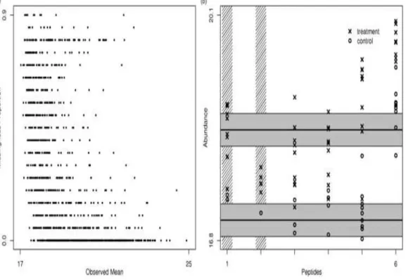
FIGURE Page 1.6 Protein quantitation. The left panel shows the proportion of missing

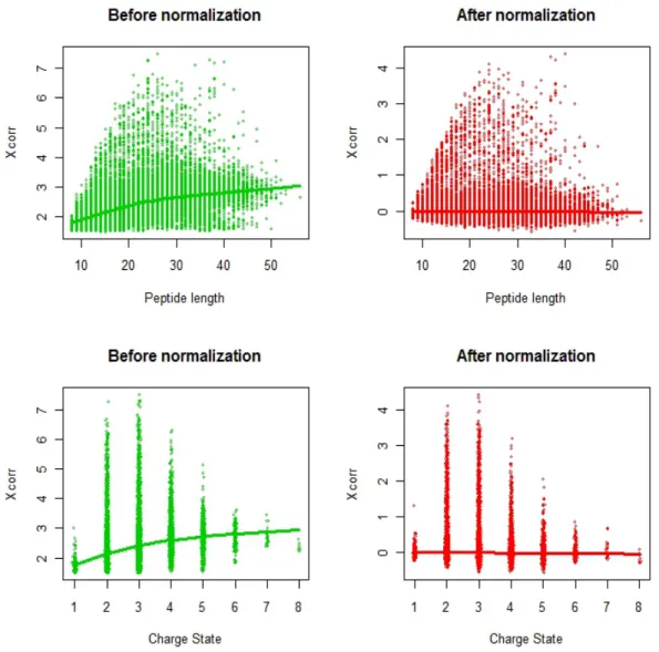
val-ues in an example data set as a function of the mean of the observed intensities for each pep- tide. There is a strong inverse relationship be-tween these, suggesting that many missing intensities have been censored. The right panel shows an example protein found to be differentially ex-pressed in a two-class human study. The protein had 6 peptides that were identified, although two were filtered out due to too many missing values (peptides 1 and 2, as indicated by the vertical shaded lines). Esti-mated protein abundances and confidence intervals are constructed from the peptide-level intensities by a censored likelihood model [21]. . . 13 2.1 Scatter plot of normalized Xcorr vs peptide length and charge state. The

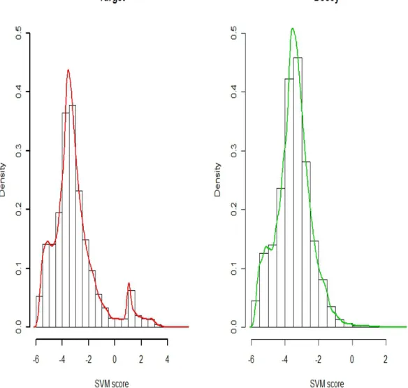
top left panel (green) is the scatter plot of Xcorr vs Peptide length before normalization and reveals a positive correlation by the fitted lowess curve. The top right panel (red) is the scatter plot of Xcorr vs Peptide length after normalization. The lowess curve fitted is essentially flat, indicating a much weaker dependency on peptide length. The bottom left panel (green) is the scatter plot of Xcorr vs charge state before normalization and reveals a positive correlation by the fitted lowess curve. The bottom right panel (red) is the scatter plot of Xcorr vs charge state after nor-malization with the fitted lowess curve relatively flat, indicating a much weaker dependency on charge state after normalization. . . 21 2.2 SVM scores. The histograms and density curves of target and decoy SVM

scores. The left panel with green curves is the distribution of the decoy SVM score and the right panel with red curves is the distribution of the target SVM score. The decoy histogram and density curve have similar shape to the incorrect SVM score in target PSMs. . . 23 2.3 Diagnostic of GEV fit on f0, the density of incorrect matching scores.

Left panel is quantile plot, the blue line is diagonal line. Right panel is density curve vs histogram. . . 27 2.4 Diagnostic of GEV fit onf1, the density of correct matching scores. Upper

Left panel is GEV quantile plot, the blue line is diagonal line. Upper right panel is Normal quantile plot, the blue line is fitted QQ-line. Bottom left panel is GEV density curve vs histogram and bottom right panel is normal density curve vs histogram . . . 28

xiv

FIGURE Page

2.5 Simplified outline of the experimental steps and work flow of the data in a typical high-throughput MS-based analysis of complex protein mix-tures. Each sample protein (open circle) is cleaved into smaller peptides (open squares), which can be unique to that protein or shared with other sample proteins (indicated by dashed arrows). Peptides are then ion-ized and selected ions fragmented to produce MS/MS spectra. Some peptides are selected for fragmentation multiple times (dotted arrows) while some are not selected even once. Each acquired MS/MS spectrum is searched against a sequence database and assigned a best matching peptide, which may be correct (open square) or incorrect (black square). Database search results are then manually or statistically validated. The list of identified peptides is used to infer which proteins are present in the original sample (open circles) and which are false identifications (black circles) corresponding to incorrect peptide assignments. The process of inferring protein identities is complicated by the presence of degenerate peptides corresponding to more than a single entry in the protein sequence database (dashed arrows) [8] . . . 30 2.6 The effect of independence assumption towards FDR estimation. Red

curve is estimated Bayesian FDR under independence assumption of PSMs on the same peptide, green curve is estimated Bayesian FDR under de-pendence PSMs assumption of PSMs on the same peptide, black curve is the true FDR lower bound. . . 36 2.7 The number of peptide identification vs the number of PSMs used in the

model at 0.05 FDR cutoff. . . 37 2.8 The number of peptide identification vs estimated FDR using top 10

PSMs candidates. The green curve is generated by our approach and the blue curve is given by PeptideProphet. The black curve is associated with the true FDR lower bound . . . 38 3.1 Plot of anchor points embedded in both samples. Left panel is for sample

one and right panel for sample two. . . 44 3.2 Histograms of Scan Number of anchor points. Left panel is for before

alignment and right panel for after alignment. . . 46 3.3 Histograms of M/Z of anchor points. Left panel is for before alignment

FIGURE Page 3.4 Histograms of Log(Peak Area) of anchor points. Left panel is for before

alignment and right panel for after alignment. . . 48 3.5 Scatter plot of Scan Number vs. M/Z on all data points. Left panel is

for before alignment and right panel for after alignment. . . 49 3.6 Scatter plot of Scan Number vs Log (Peak Area) on all data points. Left

panel is for before alignment and right panel for after alignment. . . 50 3.7 Histogram of regional p-values on Scan number. Left panel is for before

alignment and right panel for after alignment. . . 52 3.8 Heat map of regional p-values on Scan number. Left panel is for before

alignment and right panel for after alignment. . . 53 4.1 P-value histograms of simulated null peptides with shared presence

proba-bilities of 0.2,0.3,0.4,0.5 across each comparison group.The null sampling distribution is non-uniform, due to the discrete nature of the test statistic. 64 4.2 P-value histograms of simulated null peptides with shared presence

proba-bilities of 0.2,0.3,0.4,0.5 across each comparison group.The null sampling distribution is non-uniform, due to the discrete nature of the test statistic. 66 4.3 Numbers of significant single-peptide proteins versus FDR for the

pro-posed protein-level methodology, on simulated data with p1 = 0.3 and a mixture of differential presence / absence levels. The weighted FDR estimate is conservative. . . 69 4.4 Numbers of significant five-peptide proteins versus FDR for the proposed

protein-level methodology, on simulated data withp1 = 0.3 and a mixture of differential presence / absence levels. The weighted FDR estimate is conservative. . . 71 4.5 Numbers of significant mixed proteins versus FDR for the proposed

protein-level methodology, on simulated data with p1 = 0.3 and a mixture of differential presence / absence levels. Constituent peptide number varies from one to five. The weighted FDR estimate is conservative. . . 73

xvi

FIGURE Page

4.6 Numbers of significant peptides versus FDR for the proposed peptide-level methodology, on simulated data with p1 = 0.3 and a mixture of differential presence / absence. The weighted FDR estimate is conservative. 75 4.7 Numbers of significant proteins versus FDR estimates on diabetes dataset

by presence/absence based method, intensity based method and hybrid method . . . 77

1. INTRODUCTION

1.1 General Background

Proteins Proteins are the the main component of physiological metabolic path-ways of cells. Proteomics serves a important role in a systems-level understanding of biological systems since it is the large-scale study of proteins, particularly their struc-tures and functions. Mass spectrometry proteomics has become the tool of choice for qualitative and quantitative study of the proteome of an organism. Fundamental challenges in Mass spectrometry based proteomics include (i) Identification of the peptide / proteins that are present in a sample, (ii) Aligning different samples on Mass, elution time, intensity and etc. and (iii) Quantifying the abundance levels of the identified proteins after alignment. We note that protein identification and quan-titation are complementary exercises. Unidentified proteins cannot be quantified, and the confidence with which a protein was identified should perhaps be incorporated into that protein abundance estimate. All of these challenges require understanding of the biological and technological perspective as well as the development of novel statistical inference methodology.

The difficulty of protein level identification is generally caused by widespread missingness, peptide degeneracy and misidentification. The limitation of existing alignment algorithms include the lack of automated framework or quantitative sta-tistical assessment. Large-scale missingness due in part to low abundance expression contributes to the complexity of intensity-based protein quantitation. We describe a fully Bayesian hierarchical modeling approach to peptide and protein identifica-tion with False Discovery Rate constructed in a unified framework. Across different experiment samples with identified peptide/protein, “Anchor Points” are defined and

This dissertation follows the style of IEEE Transactions on Very Large Scale Integration (VLSI) Systems.

2 used to align each identified peptide automatically and a p-value is assigned to a set of aligned LC-MS runs to quantify the alignment performance. A statistical method for protein differential expression is outlined on converted presence/absence data based on a simple Binomial likelihood and a hybrid protocol is proposed to combines quantitative and presence / absence analysis and result in a single list of selected proteins with a single associated FDR.

1.2 LC-MS Proteomics

LC-MS refers to liquid-chromatography mass-spectrometry. Liquid chromatog-raphy is a technique that could be used in protein differential expression studies by separating peptides into multiple MS scans. This enables higher-resolution analysis of the resulting mass spectra. Mass spectrometry is a tool for measuring mass-to-charge ratios (M/Z) of ions.

The key components of a mass spectrometer are the ion source, mass analyzer, and ion detector (Figure 1.1). The ion source is responsible for assigning charge to each molecule. Mass analyzer measures the mass-to-charge(M/Z) ratio of each ion. The detector captures the ions and measures the intensity of each ion species. In terms of a mass spectrum, the mass analyzer is responsible for the m/z informa-tion on the x-axis and the detector is responsible for the peak intensity informainforma-tion on the y-axis. In recent years tremendous improvement in instrument performance and computational tools are used. Several MS methods for interrogating the pro-teome have been developed: Surface Enhanced Laser Desorption Ionization (SELDI) [1], Matrix Assisted Laser Desorption Ionization (MALDI) [2] coupled with time-of-flight (TOF) or other instruments, and gas chromatography MS (GC-MS) or liquid chromatography MS (LC-MS). Since GC-MS and LC-MS allow for online separation of complex samples and thus they are much more widely used in high-throughput quantitative proteomics.

Fig. 1.1. Mass spectrometry. The mass spectrometer consists of an ion source, responsible for ionizing peptides, the mass analyzer and the detector, responsible for recording m/z values and intensities, respectively, for each ion species. Each MS scan results in a mass spectrum, and a single sample may be subjected to thousands of scans.

4

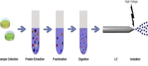
Fig. 1.2. Sample preparation. Complex biological samples are first processed to extract proteins. Proteins are typically fractionated to eliminate high-abundance proteins or other proteins that are not of interest. The remaining proteins are then digested into peptides, which are commonly introduced to a liquid chromatography column for separation. Upon eluting from the LC column, peptides are ion-ized.

Here we focus on the most widely-used bottom-up approach to quantitative MS-based proteomics, LC-MS, which has become the tool of choice for identifying and quantifying the proteome of an organism. A LC-MS-based proteomic experiment requires several steps of sample preparation (Figure 1.2), including (i) cell lysis to break cells apart and protein extraction, (ii) protein separation to spread out the collection of protein into more homogenous groups, i.e. remove contaminants and proteins that are not of interest, especially high abundance house-keeping proteins that are not usually indicative of the disease being studied, (iii) protein digestion to break intact proteins into more manageable peptide components. Once this is com-plete, peptides are further separated into a more homogeneous mixture to be ionized and introduced into the mass spectrometer. In tandem mass spectrometry (denoted by MS/MS), several of the most intense (high abundance) peaks from a parent MS (MS1) scan are automatically selected and the corresponding ions are subjected to further fragmentation and scanning. This process is repeated until all candidate peaks of a parent scan are exhausted [3], [4]. This results in a fragmentation pattern for each selected peptide, providing detailed information on the chemical makeup of the peptide.

MS/MS is preceded by LC separation and can more accurately be denoted by LC-MS/MS. High-resolution LC-MS instruments (e.g., FTICR) are very fast and can achieve mass measurements that are sufficiently accurate for identification purposes by comparing the fragmentation patterns to fragmentation spectra in a database, using software. Alignment on the scans is prerequisite for downstream quantita-tive analysis since day-to-day and run-to-run variation in the complex experimental equipment can create systematic biases. With identified peptide/protein informa-tion as well as aligned eluinforma-tion time, m/z and peak intensity, it is possible to proceed to the quantification of the abundance level of those proteins present. Each step contributes to the overall variation in the estimation and inference of the MS based proteomics.

6 1.3 Peptide/Protein Identification

To facilitate protein identification, proteins are usually separated, cleaved/digested chemically or enzymatically into fragments. Digestion overcomes many of the chal-lenges associated with the complex structural characteristics of proteins, as the re-sulting peptide fragments are more tractable chemically, and their reduced size, com-pared to proteins, makes them more amenable to MS analysis.

The first step in protein identification is the identification of the constituent pep-tides. Multiple distinct peptides can have very similar or identical molecular masses and thus produce a single intense peak in the initial MS (MS1) spectrum, making it difficult to identify the overlapping peptides. The use of separation techniques not only increases the overall dynamic range of measurements (i.e., the range of relative peptide abundances) but also greatly reduces the cases of coincident peptide masses simultaneously introduced into the mass spectrometer.

In tandem mass spectrometry (denoted by MS/MS), a parent ion possibly cor-responding to a separated peptide is selected in MS1 for further fragmentation in MS2. Resulting fragmentation spectra are compared to fragmentation spectra in a database, using software like SEQUEST [5], Mascot [6] or X!Tandem [7], see Fig-ure 1.3. PeptideProphet [8] is a widely-used for peptide identification by modeling a collection of database match scores as a mixture of a correct-match distribution and an incorrect-match distribution. The confidence of each match is assessed by its estimated posterior probability of having come from the correct-match distribution, conditional on its observed score. Improvements have been made to PeptideProphet to avoid fixed coefficients in computation of discriminant search score and utilization of only one top scoring peptide assignment per spectrum [9].

Protein identification can be carried out by rolling up peptide-level identification confidence levels to the protein level, a process that is associated with a host of issues and complexities [8]. The goal of the identification process is generally to identify as many proteins as possible, while controlling the number of false identifications at

Fig. 1.3. Peptide/protein identification. Peptide and protein identi-fication is most commonly accomplished by matching observed spec-tral measurements to theoretical or previously-observed measure-ments in a database. In LC-MS/MS, measuremeasure-ments consist of frag-mentation spectra, whereas mass and elution time alone are used in high-resolution LC-MS. Once a best match is found, one of the fol-lowing methods for assessing confidence in the match is employed: decoy databases, empirical Bayes, or expectation values.

8 a tolerable level. There are a myriad of options for the exact identification method used, including (i) the choice of a statistic for scoring the similarity between an observed spectral pattern and a database entry [7], [6], and (ii) the choice of how to model the null distribution of the similarity metric [10], [11].

In each of the above approaches, there is a statistical problem of assessing confi-dence in database matches. This is typically dealt with in one of two ways. The first involves modeling a collection of database match scores as a mixture of a correct-match distribution and an incorrect-correct-match distribution. The confidence of each match is assessed by its estimated posterior probability of having come from the correct-match distribution, conditional on its observed score [12];

The second approach to assessing identification confidence involves the use of a so-called “decoy database. A decoy database is created by scrambling the search database so that any matches to the decoy database can be assumed to be false [13], [12]. The distribution of decoy matches is then used as the null distribution for the observed scores for matches to the search database, and p-values are computed as simple proportions of decoy matches as strong or stronger than the observed matches from the search database. A hybrid approach that combines mixture models with decoy database search can also be used [13].

There are several limitations of current methods. First, many current methods are designed to evaluate the top 1 ranked PSM returned by a database searching application; this discard potential correct match that does not rank the first but among the top several highest match score. Second, recent published work [14], [15], [9] has extended the analysis from the top-ranked peptide per spectrum to a list of candidate PSMs per spectrum with independent assumption which is against the un-derlying truth that at most one PSM being correct. In Section 2, we describe a fully Bayesian hierarchical modeling approach to peptide and protein identification on the basis of MS/MS fragmentation patterns in a unified framework. Our major contri-bution is to allow for dependence among the list of top candidate PSMs, which we

accomplish with a Bayesian multiple component mixture model incorporating decoy search results and joint estimation of the accuracy of a list of peptide identifications for each MS/MS fragmentation spectrum. Peptide and protein network structure is modeled in the latent stages of the hierarchical model. We also implement a novel approach to the normalization of database searching scores to scores obtained from decoy databases, which is demonstrated to greatly improve the peptide identification performance. Finally, we propose an objective criteria for the evaluation of the FDR associated with a list of identifications at both peptide level and protein level. Using this criteria, our method is found to result in more accurate FDR estimates than existing methods like Peptide Prophet [8].

1.4 Alignment

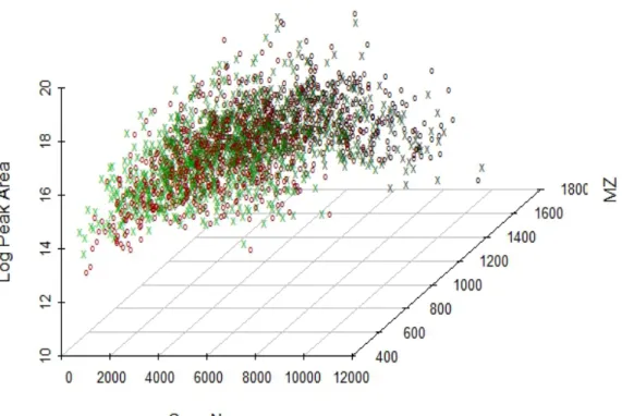
Peptides could also be identified on the basis of extremely accurate mass mea-surements and LC elution times as the output of high-resolution LC-MS instruments. When analyzing two independent samples, peptides elution times are affected by shifts relative to instrumentation effects and it is common to observe systematic dif-ferences in the elution times of similar samples on difference columns. However, the LC-MS data have added dimension of m/z and intensity information, which makes it not sufficient to provide alignment for individual peptides by only mapping the retention time coordinates between two LC-MS samples. The goal of alignment is then to match corresponding peptide features in terms of elution time, m/z and peak intensity (see Figure 1.4) from different experiment samples so that the downstream quantitation could be effectively employed.

A time warping method based on raw spectrum for alignment of LC-MS data was introduced by Bylund and others [16], which is a modification of the original corre-lated optimized warping algorithm [17]. Wang and others, implemented a dynamic time warping algorithm allowing every Retention Time (RT) to be moved. Jaitly, et al. [18] introduced a non-linear alignment technique that uses a dynamic time

10

Fig. 1.4. Two sample of scans before alignment, red dots represent sample 1 and green dots represent sample 2. X axis is ScanNum (equivalent to elution time), Y axis is M/Z and Z axis is Log (Peak intensity).

warping approach at a feature level. Radulovic and others [19] performed alignment based on (m/z,RT) values of detected features by dividing the m/z domain into sev-eral intervals and fitting different piece-wise linear time warping functions for each m/z interval and then applying a “wobble” function to peaks and allow peaks to move. Palmblad, et al. [20] applied a genetic algorithm to establish an alignment warping function by using peptide elution times from MASCOT output to define anchor points between two datasets.

All of these alignment techniques still suffer from either not taking m/z and peak intensity information into account or manually inappropriate division of m/z domain or incorrect parameterization of warping function as well as lacking a useful metric for scoring an alignment between two datasets. To score alignments, a ground truth is required to assess the accuracy of an alignment by establishing links between datasets via database searches to find the same peptide present in two datastes. (Simply matching two features based on mass and elution time alone is not very supportive).

Our approach in Section 3 uses “Anchor points” found between two samples to align all the individual scan in the second sample and provides a framework to quantitify the alignment, that is, assigning a p-value to a set of aligned LC-MS runs to assess correctness of alignment. In our method, for different experiments, we have the elution time, mass over charge (m/z) value, peak intensities, peptide information for each of the thousands of scans in the SEQUEST search output. A feature is treated as an “anchor point” if it corresponds to very high confidence identification to the same peptide in all samples (in addition to meeting other quality standards). The anchors can be relied upon with very high confidence as being paired across samples. As such, they can be used as the basis of an alignment algorithm, as well as for assessing the performance of an alignment algorithm.

12

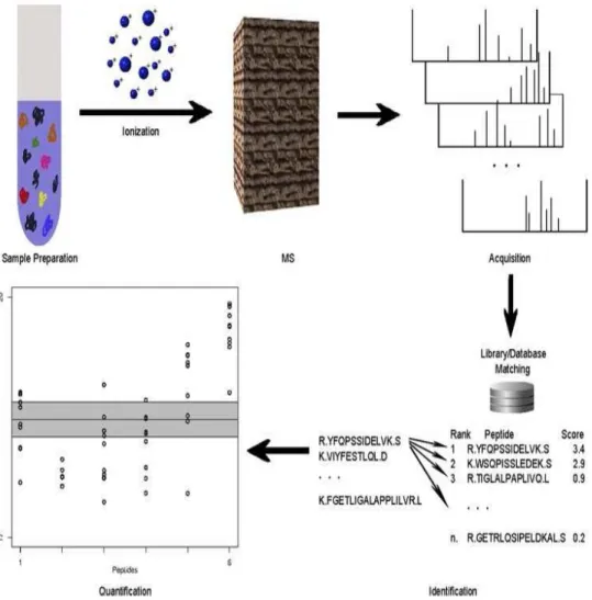
Fig. 1.5. Overview of LC-MS-based proteomics. Proteins are ex-tracted from biological sam- ples, then digested and ionized prior to introduction to the mass spectrometer. Each MS scan results in a mass spectrum, measuring m/z values and peak intensities. Based on observed spectral information, database searching is typically em-ployed to identify the pep- tides most likely responsible for high-abundance peaks. Finally, peptide information is rolled up to the protein level, and protein abundance is quantified using either peak intensities or spectral counts

Fig. 1.6. Protein quantitation. The left panel shows the proportion of missing values in an example data set as a function of the mean of the observed intensities for each pep- tide. There is a strong inverse relationship between these, suggesting that many missing intensities have been censored. The right panel shows an example protein found to be differentially expressed in a two-class human study. The pro-tein had 6 peptides that were identified, although two were filtered out due to too many missing values (peptides 1 and 2, as indicated by the vertical shaded lines). Estimated protein abundances and confi-dence intervals are constructed from the peptide-level intensities by a censored likelihood model [21].

14 1.5 Protein Quantitation

Quantitative proteomics is concerned with quantifying and comparing protein abundances in different conditions (Figure 1.5). Once a list has been constructed of the proteins believed to be present in the sample and the peak intensity is aligned, the next task is to quantify the abundance of the proteins. Protein abundance infor-mation is contained in the set of peaks that correspond to the protein’s component peptides. Peak height or area is a function of the number of ions detected for a par-ticular peptide, and is related to peptide abundance [22]. Regardless of the specific technology used to quantify peptide abundances, statistical models are required to roll peptide level abundance estimates up to the protein level. Intensity based pro-cedures for differential protein expression are naturally constructed in the context of regression or ANOVA, or as a “rollup” problem [23].

However, intensity-based procedures are challenged by the presence of widespread missing intensities, which are prevalent in MS-based proteomic data. In fact, it is common to have 20% -40% of all attempted intensity measures missing. Abundance measurements are missed if, for example, a peptide was identified in some samples but not in others, see Figure 1.6. This can happen partially due to the low abun-dances of present peptides, which is essentially a censoring mechanism [24]. With standard regression or ANOVA procedures, peptides with missing values must either be removed from the analysis, or their missing values must be imputed. There will typically be very few peptides with no missing values, so filtering peptides in this way results in a much less informative data set. The simple imputation routines are not appropriate [25] since the vast majority of missing values are the results of censoring of absent or low-abundance peptides. This complicates intensity-based quantitation, as simple solutions will tend to be biased. For example, analysis of only the observed intensities will tend to overestimate abundances and underesti-mate variances. Simple imputation routines like row-means or k-nearest-neighbors suffer from similar limitations. Parametric imputation and other specialized

method-ology can be employed to enable intensity-based inference with lessened information loss [21]. However, some information loss is inevitable. In particular, “one-state” (or nearly so) peptides, those for which there are many observed intensities in one com-parison group but few in another comcom-parison group, are of great biological interest but not amenable to an intensity-based analysis and filtered out in intensity-based analysis. Statistical models are needed to address these issues, as well as to handle the peptide-to-protein rollup [21], [26], see Figure 1.5.

In Section 4, we propose a “presence / absence” analysis, in which peak intensities are digitized into binary measurements depending on whether a peak was observed or not. Data collected in our laboratory does not necessarily have MS/MS frag-mentation data associated with it, instead being obtained according to the Accurate Mass and Time (AMT) tag pipeline [27]. We also present a hybrid analysis protocol that consists of two stages: (i) intensity-based analysis, and (ii) a presence / absence analysis. The results of each are merged to create a single collection of “interest-ing” proteins, to which we use novel methodology to apply a single FDR. For the proposed hybrid analysis protocol, we demonstrate the following: (i) Resulting FDR estimates are conservative, (ii) One-state proteins are consistently selected as differ-entially expressed, and (iii) The number of differdiffer-entially expressed proteins selected at a specified FDR exceeds that either intensity-based or presence / absence analysis alone.

16 2. A BAYESIAN HIERARCHICAL MODEL FOR PEPTIDE / PROTEIN

IDENTIFICATION BY LC-MS/MS.

2.1 Introduction

A fundamental challenge in quantitative mass spectrometry (MS)-based pro-teomics is the identification of peptides and proteins that are present in a sample. This is typically carried out by comparing observed features to entries in a database of theoretical or previously-identified peptides (figure on page 7). In tandem mass spectrometry (denoted by MS/MS or MSn_{), fragmentation spectra are obtained for}

each subset of observed high-intensity peaks and compared to fragmentation spec-tra in a database, using software like SEQUEST [5], Mascot [6], or X!Tandem [7]. Alternatively, high-resolution MS instruments can be used to obtain extremely ac-curate mass and time (AMT) measurements, and these can be compared to AMT measurements in a database [28]. In either case, a statistical assessment of the level of confidence for each identification is desired; for the purposes of this section, we fo-cus on peptide-spectrum matches (PSMs) and MS/MS. Protein identification can be carried out by rolling up peptide-level identification confidence levels to the protein level [8], or by the simultaneous modeling of peptides and proteins using hierarchical models [29]. The goal of the identification process is generally to identify as many features as possible, while controlling the number of false identifications at a toler-able level. There are a myriad of options for the exact identification method used, including (i) The choice of a statistic for scoring the similarity between an observed spectral pattern and a database entry, and (ii) The choice of how to model the null distribution of the similarity metric [10], [11].

There are several limitations of current methods. First, many current methods are designed to evaluate the top 1 ranked PSM returned by a database searching

application. Recent published work [14], [15], [9] have extended the analysis from the top 1 ranked peptide per spectrum to a list of candidate PSMs per spectrum. But existing approaches have made the assumption that multiple PSMs in the list of candidate matches are independent. In complex samples, it is possible that multiple peptides may give rise to very similar fragmentation patterns. However, it is reason-able to expect that there is only one correct database entry that matches a specific fragmentation pattern, in which case the PSMs in a list of top candidate matches will not be independent. Our experiments suggest that the independence assump-tion may lead to underestimated false discovery rates among identified peptides, see figure on p. 36 in section 2.3.

In this section, we describe a fully Bayesian hierarchical modeling approach to peptide and protein identification on the basis of MS/MS fragmentation patterns in a unified framework. Our major contribution is to allow for dependence among the list of top candidate PSMs, which we accomplish with a Bayesian multiple component mixture model incorporating decoy search results and joint estimation of the accuracy of a list of peptide identifications for each MS/MS fragmentation spectrum. Peptide and protein network structure is modeled in the latent stages of the hierarchical model. Our model can incorporate arbitrary collections of discriminant features for quantifying match quality; examples include scores from different search applications like XCorr and Sp from SEQUEST, hyperscore and E-value from X!tandem, and other auxiliary discriminant information. We also implement a novel approach to the normalization of database searching scores by utilizing scores obtained from decoy databases, which is demonstrated to greatly reduce the dependency among discriminant features, see figure on page 21. Finally, we propose an objective criteria for the evaluation of the FDR associated with a list of identifications at peptide level. Using this criteria, our method is found to result in more accurate FDR estimates than existing methods like PeptideProphet [11].

18

2.2 Methods

2.2.1 Experiments

The data we used came from 5 quality-control LC-MS/MS runs of Shewanella oneidensis, prepared by and run at the Pacific Northwest National Laboratory. For each sample, we have SEQUEST output for use in the peptide and protein identifi-cation process.

2.2.2 Peptide and Protein Identification by Database Search

The identification of peptide assignments to MS/MS spectra is primarily based on database search scores computed by different search engines together with var-ious peptide-specific properties. Most database search approaches employ a score function to measure the similarity between peptide MS/MS spectra and theoreti-cal spectra constructed for each peptide in the searched protein sequence database. Different search engines such as SEQUEST [5], X!tandem [7] and Mascot [6] adopt different scoring systems. For example, SEQUEST computes a correlation score be-tween a normalized MS/MS spectrum and a unit-intensity fragmentation model and corrects it by an estimation of the background. X! Tandem defines a score function based on the shared peak count approach and calculates an “expectation value” for each peptide assignment. Mascot computes a probability-based score called the ion score (often referred to simply as Mascot score) using the Mowse scoring algorithm. Other than database search scores, some additional measurements might also contain useful discrimination information, such as the difference (dT) between the observed and predicted elution time (such as the “Normalized Elution Time” (NET) [30]), the difference between the measured and calculated peptide mass (dM), the frac-tional difference between current and second best Xcorr δCn, the Number of Tryptic

measurement “multi-protein”. All these features are potentially informative for dis-tinguishing between correct and incorrect PSMs. Ideally, incorporating all available discriminant features should greatly improve tandem mass spectrum identification.

In this section, we consider a target-decoy search strategy, which has been used successfully in peptide and protein identification analysis [10]. Decoy databases are usually created by reversing or randomly shuffling the target peptide sequences. The distributions of some PSM attributes (e.g., peptide length, elution time, charge state, database search score) from a decoy database search are assumed to be the same as those of false identifications from target database search. And incorrect PSMs from decoy sequences are assumed to be equally as likely as those from target sequences. Based on these assumptions, target-decoy search strategies have been successfully used to distinguish correct identifications from incorrect ones [14], [31] and estimate confidence levels for peptide assignments [32].

In some cases, database search scores should be transformed prior to analysis. For example, consider the SEQUEST primary score, XCorr, a measure of the cor-relation between observed and theoretical fragmentation spectra. XCorr is highly dependent on peptide length and precursor ion charge state (see, e.g., [11] and [33]). In particular, long peptides tend to have higher XCorr values than short peptides, due simply to more frequent random matching of observed and theoretical spectral features. Precursor ions with different charge states also have different probabili-ties of having random hits, yielding shifts in the distributions of XCorr scores. To alleviate this problem, PeptideProphet normalizes XCorr based on a deterministic transformation, which is a function of peptide length. The transformed XCorr is denoted as XCorr0. Due to the existence of charge state effects in the transformed XCorr, PeptideProphet models each charge state separately.

We propose a novel approach to the normalization of discriminant scores, utilizing the scores observed for matching to the decoy database. As an example, assuming the top R ranked decoy XCorr scores for each spectrum are available, we

normal-20 ize the target XCorr scores by subtracting the average XCorr scores for the top R

ranked decoy PSMs. In what follows, we let XCorr∗ denote the decoy-normalized version of XCorr. The underlying assumption of this transformation is that peptide length dependence and charge state dependence in decoy XCorr scores can be used to approximate the corresponding dependencies in target XCorr scores.

This transformation is easy to implement yet effective to reduce the sequence length dependence and charge state dependence. Figure 2.1 clearly suggests that the distribution of the normalized XCorr score shows much weaker dependence on peptide length and charge state. In addition, XCorr∗ is by nature a measurement of relative XCorr score defined for the top R ranked target PSMs. XCorr∗ alone offers comparable discrimination information with both XCorr0 and δCn. Because of these

desired properties, we employ XCorr∗ as a primary SEQUEST searching score in the subsequent analysis.

When multiple (transformed) discriminant features are available, one common strategy is to combine (a subset of) them into a single discriminant score for simplifi-cation purposes, which can greatly relieve the complexity of the subsequent mixture distribution specification. There are many dimension reduction and classification tools to choose from, including linear discriminant analysis (LDA), principle com-ponent analysis (PCA), logistic regression and support vector machines (SVM). For example, PeptideProphet employs LDA to derive a scaler score “fval” from a num-ber of database search scores. All other information together with “fval” is modeled in an unsupervised or semi-supervised fashion at subsequent steps [11], [31], [13]. Percolator uses a semi-supervised machine learning method that iteratively trains a SVM classifier containing all discriminant features [14], where each PSM is assigned a decision score.

In this section, we employ a similar approach as Percolator, using a radial basis function (RBF) as the kernel function to train a semi-supervised SVM in a dynamic fashion. The top 1 ranked target and all decoy discriminant features are used as

Fig. 2.1. Scatter plot of normalized Xcorr vs peptide length and charge state. The top left panel (green) is the scatter plot of Xcorr vs Peptide length before normalization and reveals a positive corre-lation by the fitted lowess curve. The top right panel (red) is the scatter plot of Xcorr vs Peptide length after normalization. The lowess curve fitted is essentially flat, indicating a much weaker de-pendency on peptide length. The bottom left panel (green) is the scatter plot of Xcorr vs charge state before normalization and re-veals a positive correlation by the fitted lowess curve. The bottom right panel (red) is the scatter plot of Xcorr vs charge state after normalization with the fitted lowess curve relatively flat, indicating a much weaker dependency on charge state after normalization.

22 the training dataset, and the combined discriminant score is then calculated for all of the top R target PSMs using the SVM function derived by the training dataset. Figure 2.2 shows the distributions of target and decoy SVM scores. The bi-modality of the distribution of target scores clearly suggests that target PSMs are comprised of a mixture of correct and incorrect PSMs, suggesting the use of mixture modeling. Also, the distribution of scores assigned to decoy PSMs is very similar to the distri-bution for incorrect target scores. We note that SVM is primarily used as for scoring purposes, rather than as an ultimate classifier or validation tool in the identification process. There are many other scoring approaches for classification tools that might achieve better combined discriminant scores. It is also possible to apply SVM to database search scores only and then specify a multivariate mixture distribution for the database search score combined with other discriminant information. However, it is beyond the scope of this section to discuss and compare all of these possibilities.

2.2.3 Model

Many existing approaches to peptide identification are designed to model the top 1 scoring PSM for each spectrum only (ranked according to a certain scoring cri-terion). The combined discriminant score (or multiple discriminant scores) can be modeled as a parametric or semi-parametric mixture distribution with two compo-nents representing correct and incorrect identifications, respectively. In a Bayesian framework, the posterior probability that a PSM belongs to the correct-match dis-tribution can be used as a statistical measure of confidence.

In this section, we present a model that accommodates a list of potential matches (PM) for each spectrum. We might, for instance, wish to use the top 10 ranked PSMs returned by a particular searching application, or a list of unique top 1 ranked PSMs based on multiple search algorithms. In practice, it is expected that many correct peptide assignments are ranked slightly lower than the top 1 ranked PSM based on an algorithm-derived score. Our goal is to take advantage of the information for all

Fig. 2.2. SVM scores. The histograms and density curves of target and decoy SVM scores. The left panel with green curves is the distri-bution of the decoy SVM score and the right panel with red curves is the distribution of the target SVM score. The decoy histogram and density curve have similar shape to the incorrect SVM score in target PSMs.

24 available discriminant features and peptide protein grouping information to bump correct PSMs up the ranking list. This would enable us to discover more correct PSMs than approaches based on single best PSM scores alone.

In this approach, database search algorithms such as SEQUEST are employed to filter out a list of candidate PSMs and calculate their corresponding discriminant features. The subsequent statistical analysis serves as a second search step to find the most likely match within the candidate list based on their estimated confidence levels. Although several existing approaches also consider multiple peptide assign-ments per spectrum [14] and [15], they typically impose independence assumption in the correctness for PSMs in the same candidate list. However, this assumption may not hold in practice and could render higher false discovery rate. For example, given that one candidate PSM has a significantly higher chance to be correct, the probability that other candidates are also correct should be low.

We relax the independence assumption in our approach. A multiple component mixture model is proposed in the first stage to jointly infer the correctness of every candidate PSM for each spectrum based on the combined discriminant score. Since the prior probabilities of being correct matches are connected to the unobserved pres-ence/absence of peptides and proteins. We employ a Bayesian hierarchical modeling approach that models peptide and protein network information in the latent layers. Some common complexities in peptide/protein identifications are also addressed in our model.

The First Stage: a Multi-component Mixture Model for Discriminant Scores We introduce some notations first. Assume we haveK experimental spectra, each of which is assigned a PM list with Rk PSMs, e.g., the top R ranked PSMs from

SEQUEST. Letsr

k denote the combined discriminant score of therth match for

containing scores for those R matches, s1:Rk\r = (sk,1, sk,2, ..., sr−1, sr+1, ..., sk,Rk),

denote a vector containing scores for all candidates except for the rth match. We introduce a Rk + 1 dimensional component label vector Zk, where the rth

element of Zk, Zk,r = (Zk)r, is a binary indicator. We assume there is at most

one correct PSM in the PM list for each spectrum. Zk,Rk+1 = 1 indicates none

of the Rk matches in the PM list being correct. For r from 1 to Rk, Zk,r = 1

indicates the rth PSM is the only correct match in the PM list for spectrum k. Define pk = (pk,1, ...., pk,Rk+1)

0

, where pk,r = P r(Zk,r = 1). Then

PRk+1

r=1 pk,r =

1. The imposition of this restriction connects the probabilities of being correct for multiple PSMs assigned to the same spectrum. It enables us to compute the peptide probabilities for one candidates while taking into account information from other matches in the same PM list.

Let f1 denote the density function for score with correct-match and f0 denote the density function for score with incorrect-match. Conditional on the label vector

Zk, discriminant scores are assumed to be independently following the distribution

shown below, P r(sk|Zk) = Rk Y r=1 f1(sk,r)I(Zk,r=1)f0(sk,r)I(Zk,r=0)

Integrating out the latent label vectorZ, it yields a mixture distribution with Rk+ 1

components for target discriminant scores.

s(_k,target_1:R ) k ∼ Rk X r=1 I(Zk,r = 1)f1(s (target) k,r )f0(s (target) k,{1:Rk}\r) +I(Zk,Rk+1 = 1)f0(s (target) k,1:Rk ) ∼ Rk X r=1 pk,rf1(s (target) k,r )f0(s (target) k,1:Rk\r) +pk,0f0(s (target) k,{1:Rk})

Recall that distribution of decoy scores provides a satisfying approximation to the distribution of scores from incorrect target matches. Incorporating decoy scores

26 in the model could obtain improved robustness in the estimation of f0 and hence better discrimination for target PSMs. The model is:

sk,1:R(incorrect) ∼ f0(s (decoy)

k,1:R ) (2.1)

The choice of functional forms for f0 and f1 will depend on the specific method used to derive the combined database search score. In our case, we used Xcorr, Rank Sp, NTE, “multi-protein” and charge state as the covariates for the combined

SVM score, which greatly simplifies the task of mixture distribution specification. We model f0 using the generalized extreme value (GEV) distribution with location parameter µ0, scale parameterσ0 and shape parameter ξ0. The GEV distribution is the limit distribution of properly normalized maxima of a sequence of independent and identically distributed random variables. It is commonly used as an approxima-tion to model the maxima of long (finite) sequences of random variables. In our case, the combined scores for PSMs in the PM list are among the highest of the entire database, making GEV distribution a natural choice for f0. The diagnostic analysis also showed that the GEV distribution can describe the shape of combined discrimi-nant score well, see Figure 2.3. Similarly, empirical exploration study suggests using a GEV density to modelf1 rather than a normal density, with location paramterµ1, scale parameter σ1 and shape parameterσ0 to be estimated, see Figure 2.4.

Latent Stages: Prior Models for Peptide and Protein Network

In tandem MS/MS dataset, peptide level and protein level information are nat-urally connected in a hierarchical structure. Figure on page 29 briefly illustrates the work flow of the LC-MS/MS experiment and the peptide and protein network information. As is shown in this figure, each protein can generate a list of peptides and some peptides can be generated by multiple proteins. If peptide j is correctly identified and unique to protein i, then protein i must be present in the sample,

Fig. 2.3. Diagnostic of GEV fit onf0, the density of incorrect match-ing scores. Left panel is quantile plot, the blue line is diagonal line. Right panel is density curve vs histogram.

28

Fig. 2.4. Diagnostic of GEV fit on f1, the density of correct match-ing scores. Upper Left panel is GEV quantile plot, the blue line is diagonal line. Upper right panel is Normal quantile plot, the blue line is fitted QQ-line. Bottom left panel is GEV density curve vs his-togram and bottom right panel is normal density curve vs hishis-togram

which in turn implies higher chance of detecting the sibling peptides of peptide j in the experiment.

Many conventional approaches follow a two step procedure to assess peptide and protein confidence levels, in which peptide confidence levels are obtained from a like-lihood model for discriminant score(s) in the first step and protein confidence levels are estimated based on the peptide-level results. Apparently, by borrowing strength from peptide/protein grouping information, an integrated analysis can produce more accurate assessment for peptide and protein identification [29].

There are two major complexities that need to be addressed in modeling peptide and protein network. The first complexity is called “degeneracy” problem [11]. If a peptide can be generated by multiple proteins, then it adds ambiguity into protein identification since we only know at least one of these proteins must be present. Few work has been done to address this problem. Another common complexity is that multiple spectra with different scores can be assigned to the same peptide, again, adding ambiguity in assessing confidence levels for peptides with multiple spectra. This complexity primarily arise from two different situations: i) tandem MS/MS technique can generate repeated fragment ion spectra [34], which are mostly likely to be assigned to the same peptide; ii) a false identified peptide can be assigned to multiple spectra due to random matches. Many conventional approaches only keep the maximum score for analysis, leading to two potential limits. First, it ignores information from other spectra that may help with peptide identification. For exam-ple, if multiple PSMs associated with the same peptide are due to repeated spectra, larger number of repeated spectra should imply higher peptide confidence level. Sec-ond, if multiple PSMs associated with the same peptide are due to random matches, ignoring information from lower scores can possibly yield overestimated peptide con-fidence level since a false identified peptide can be assigned with a high score by chance. Apparently, modeling multiple PSMs to the same peptide would require distinguishing those two situations. Frank etal. [34] propose a clustering approach

30

Fig. 2.5. Simplified outline of the experimental steps and work flow of the data in a typical high-throughput MS-based analysis of com-plex protein mixtures. Each sample protein (open circle) is cleaved into smaller peptides (open squares), which can be unique to that protein or shared with other sample proteins (indicated by dashed arrows). Peptides are then ionized and selected ions fragmented to produce MS/MS spectra. Some peptides are selected for fragmen-tation multiple times (dotted arrows) while some are not selected even once. Each acquired MS/MS spectrum is searched against a sequence database and assigned a best matching peptide, which may be correct (open square) or incorrect (black square). Database search results are then manually or statistically validated. The list of identi-fied peptides is used to infer which proteins are present in the original sample (open circles) and which are false identifications (black cir-cles) corresponding to incorrect peptide assignments. The process of inferring protein identities is complicated by the presence of degener-ate peptides corresponding to more than a single entry in the protein sequence database (dashed arrows) [8]

to identify redundant spectra and replace each cluster with a single representative spectrum. We believe this clustering type of approaches followed by database search applications can greatly reduce the number of repeated spectra. However, it may not be able to find all redundant spectra.

Bayesian hierarchical model is a convenient choice that allows us to incorporate different levels of information in a unified framework. We describe models with multiple latent layers to describe peptide and protein network. Models at latent stage is connected to the mixture model in the first stage through the prior model for pZ|Y. In this section, we describe a model based approach to address the two

major complexities discussed above.

We first introduce peptide level indicator and protein level indicator. Let Xi

denote a binary indicator such that Xi = 1 if protein i is present in the sample

and detected, and 0 otherwise. Let Yj be a binary indicator such that Yj = 1 if

peptide j is present in the digested sample and detected, and 0 otherwise. Let

pep(k, r) denote the peptide index number of the rth PSM for spectrum k. Recall

Z is a Rk+ 1 dimensional component label vector Zk, where the rth element of Zk

indicating whether the rth match is correct for r ≤ Rk. Conditional on peptide

indicator Y, PSM indicators Z and protein indicatorsX are independent. Based on peptide and protein network information, we build three models in the latent stages,

P r(Z|Y),P r(Y|X) and P r(X) respectively.

The Second Stage: Pr(Z|Y)

Conditional on a peptide is absent, it is reasonable to assume that all PSMs that are matched to this peptide are incorrect. If a peptide is correctly detected and only one PSM is matched to it, we assume that PSM is correct. If a peptide is correctly detected but have multiple hits, it is possible that some hits are due to

32 random matching. Those assumptions become the major guideline for us to model the conditional probability, P r(Z|Y).

P r(Z|Y) = P r(Zk,r = 1|Ypep(k,r)) =

τk,r Ypep(k,r)=1 0 Ypep(k,r)=0

(2.2)

whereτk,r is the conditional probability that therth match for spectrumk is correct

given peptide pep(k, r) is present. As we discussed above, if multiple PSMs assigned to the same peptide originate from repeated spectra, we expect their conditional probabilities of being correct are consistently close to 1. If PSMs are assigned to the same peptide by random chance, we expect their conditional probabilities of being correct take a much smaller value than 1. We use DM, the difference between observed Mass and theoretical Mass as a major covariate to distinguish between repeated spectra and random matches. When a PSM is unique to a peptide, DM = 0. We expect its conditional probability to be 1 or close to 1. In other cases, we expect that the larger the absolute deviation is, the more likely the PSM is assigned due to random matching. A logistic regression or Probit model using DM as covariate information is desired to model the conditional probability τk,r. For simplicity, we

pick a threshold C for DMk,r and assume a prior model for τk,r as follows:

τk,r =

1 |DMk,r| ≤C

τ |DMk,r|> C

(2.3)

Based on exploratory data analysis on previously observed NET combined with expertise’s suggestion, we choose C = 0.5 as a threshold. τ is an unknown parame-ter. We assign a prior distribution on this parameter and estimate it using MCMC approach (see Appendix for details).

The Third Stage: Pr(Y|X)

If a protein is absent, it is reasonable to assume that none of its constituent peptides can be correctly detected. If a protein is present, it is common that only

a subset of its constituent peptides can be correctly identified. In the case of ’de-generacy’, a peptide can be generated by different proteins. Again, we follow those information to specify the conditional probability model for peptide indicators Y

given protein indicators X.

We letπi,j =P r(Yj = 1|Xi = 1) denote the probability that peptidej is correctly

identified conditional on its parent proteini being present. Let Cj denote the set of

proteins that could potentially generate peptide j. Notice that the probability that peptide j is present in the digested sample is equal to the probability that at least one protein in Cj generates it.

We have

P r(Yj|X) = 1−

Y

i∈Cj

(1−πi,j)Xi (2.4)

This conditional probability πi,j might depend on certain peptide sequence

spe-cific information, such as amino acid content, charge, hydrophobicity and polarity (see [29]). Ideally, incorporating those covariates that contain information about the observability of peptides can help us accurately estimate peptide and protein probabilities. Again, a logistic regression or Probit model can be a natural choice to incorporate those relevant explanatory variables in a prior model for πi,j. Due to

the lack of those measurements in our data, we simply assume πi,j = π, a constant

unknown parameter which has prior information assigned before MCMC steps.

The Fourth Stage: Pr(X)

Finally, we assume the prior model for the presence of protein i is a Bernoulli distribution, i.e., P(Xi = 1) = qi. Here qi is the prior probability that protein

i is present. Again, prior knowledge on the presence/absence status of proteins can be naturally incorporated in the prior model for qi. For example, if organism

34 hierarchical framework that reflects protein/organism grouping information. Again, due to the lack of this information in our study, we simply assume qi =q, a constant

unknown parameter that has prior information assigned before MCMC steps.

2.2.4 Bayesian Implementation and Bayesian False Discovery Rate

We employ MCMC methods to do the model fitting. We begin with prior spec-ifications for the parameters. Recall that we have unknown parameters (µ0, σ0, ξ0) in the GEV distribution f0, (µ1, σ1, ξ1) in the GEV distribution f1, τ, π and q in the latent stage models. Vague normal priors are assigned to the location parameter

µ0, µ1, shape parameter ξ0, ξ1, and an inverse gamma priors are assigned to σ0, σ1. We also assign Beta(1,1), i.e., uniform distribution on [0,1], to the parameters π,τ

and q.

Posterior inference for the model parameters is completed using Gibbs sampling [35] with Metropolis-Hastings updating [36]. With the above hierarchical model and prior setup, all the conditional distributions turn out to be of known standard except for the GEV parameters inf0 andf1. (µ0, σ0, ξ0),(µ1, σ1, ξ1) are then updated using Metropolis steps. Typically, random walk Metropolis with normal proposals is adopted. The detailed MCMC steps are given in Appendix.

In particular, we collect posterior samples of the latent peptide indicators Yj.

The posterior correctness probability for each peptide is estimated by the posterior sample proportion ofYj. The correctness probability for each protein is obtained in a

similar way. The associated posterior error probability (PEP, also referred to as local false discovery rate) is defined as the probability of being incorrect, simply calculated by subtracting posterior probability from one. For a given probability threshold pc,

peptides with PEPs lower than pc are decided to be positive identifications. The

Bayesian FDR (see [37] and [32]) associated with the above decision is estimated by the average PEPs that are below pc.

F DR(pc) =

P

P EP <pcP EP

#{P EP < pc}

A similar approach is easy to be applied to protein posterior PEPs. The Bayesian FDR could be used to assess the protein level identifications by our approach.

2.3 Results

Our identification approach is applied to the SEQUEST output on the Shewanella data described in section 2.1. The independence assumption among PSMs causes un-derestimated FDR, i.e. over-estimated number of identification at a specific FDR cutoff, which confronts with the rule of conservative estimation. Figure 2.6 shows that, compared with the true FDR lower bound, there are more identified pep-tides at the same Bayesian FDR estimated under PSMs independence assumption (red curve), which obeys the conservative rule for FDR estimation. Meanwhile, the Bayesian FDR estimated under PSMs dependence assumption (green curve) shows its conservative character.

The number of PSMs incorporated into the model–R has an impact on peptide identification. Figure 2.7 shows the positive trend between the number of identified peptides versus R–the number of top PSMs candidates utilized in the model, at a specific FDR cutoff 0.05. The same trend maintains at different FDR cutoffs.

Our approach that models the top 10 PSMs, which identifies more peptide fea-tures than PeptideProphet under most of the circumstances except for estimated FDR below 0.02, see Figure 2.8.

36

Fig. 2.6. The effect of independence assumption towards FDR esti-mation. Red curve is estimated Bayesian FDR under independence assumption of PSMs on the same peptide, green curve is estimated Bayesian FDR under dependence PSMs assumption of PSMs on the same peptide, black curve is the true FDR lower bound.

Fig. 2.7. The number of peptide identification vs the number of PSMs used in the model at 0.05 FDR cutoff.

38

Fig. 2.8. The number of peptide identification vs estimated FDR using top 10 PSMs candidates. The green curve is generated by our approach and the blue curve is given by PeptideProphet. The black curve is associated with the true FDR lower bound