Using Self Organizing Maps on compositional data.
Joaqu´ın A. Cort´es1 and Jos´e Luis Palma2
1Department of Geology, University at Buffalo. Buffalo, USA;[email protected] 2
Geological and Mining Engineering and Sciences, Michigan Tech University, Michigan, USA.
Abstract
Self–organizing maps (Kohonen 1997) is a type of artificial neural network developed to explore patterns in high–dimensional multivariate data. The conventional version of the algorithm involves the use of Euclidean metric in the process of adaptation of the model vectors, thus rendering in theory a whole methodology incompatible with non–Euclidean geometries.
In this contribution we explore the two main aspects of the problem:
1. Whether the conventional approach using Euclidean metric can shed valid results with compositional data.
2. If a modification of the conventional approach replacing vectorial sum and scalar multiplication by the canonical operators in the simplex (i.e. perturbation and powering) can converge to an adequate solution.
Preliminary tests showed that both methodologies can be used on compositional data. However, the modified version of the algorithm performs poorer than the conventional version, in particular, when the data is pathological. Moreover, the conventional ap-proach converges faster to a solution, when data is “well–behaved”.
1
Introduction
The Self Organizing Maps (SOM) algorithm is an unsupervised neural network with properties of vector quantization and vector projection algorithms (Kohonen 1997). The basic SOM works as aclustering method by unsupervised competitive learning that adapts the network parameters according to the presentation of new input data to the network. This adaptation is based on pre–defined learning rules that are derived from a measure of dissimilarity and a neighborhood function which dictates the topology of the map. One of the main results of the clustering is the reduction of the amount of data and the formation of a topologically ordered mapping, be means of a nonparametric regression, of the data. This ordered mapping gives the SOM the capability of aprojection method by showing the input space into a low dimensional (commonly one or two dimensions) regular array of model vectors (neurons). In addition, the process in which such mapping is formed allows a non–linear regression and projection of the data. The amount of applications carried out using SOM is vast; see the examples in Kohonen (1997) and references therein.
The main goal of this contribution is to explore the implementation of the SOM algorithm with compositional data in the simplex. Through experiments using compositional data of three com-ponents, it is shown that SOM yields satisfactory results with standard Euclidean metric. Further-more, in the examples presented herein, the results obtained using Aitchison’s perturbation and powering exhibit a poorer representation of the data.
2
SOM generic algorithm
The SOM basic algorithm consists of the following steps:
Pre-processing Preparation of the data (i.e. any kind of normalization). Each data pointxi∈Q,
in whichQ⊆Rn, these vectors are calledinput vectors. Qmight not be a sub–vector space
ofRn.
Initialization set parameters: learning rate and neighborhood parameter, number of model vec-tors (N), and number of iterations; locate model vectors.
Training Loop:
1. Pick randomly an input samplexi
2. Find the best matching unit (BMU) among theN model vectors
3. Adapt the BMU and neighbor model vectors based on the learning rate and neighbor-hood function
4. Go to 1
2.1
The model vectors and their neighborhood
After any previous preparation of the data, a setwij of “weight”, “prototype” or “model vectors”,
often called neurons because of their biological analogue (Hertz, Palmer, and A.S. 1990), needs to be defined. The number of model vectors is arbitrary, but for a practical computation they typically are around 10% of the input vectors (Kohonen 1997). There are several ways to create the models vectors depending on how much is known from the data. Commonly, they are defined on an equi–spaced grid generated using the orientation of the two main eigenvectors from the Principal Component Analysis of the data, although it is also possible to define them randomly (Kohonen 1997). Next, a set of “connections” (the topology) between the model vectors is defined, usually linear (2 neighbors), rectangular (4 neighbors) or hexagonal (6 neighbors).
2.2
The Best matching Unit and the adaptation function
The search for the BMU is performed under a specific dissimilarity relationship. In the original SOM, one of the most common dissimilarity relation occupied is the Euclidean distance (Equation 1): de(x, y) = v u u t n X i=1 (xi−yi)2 (1)
and the adaptation is performed by means of an approximation over the straight line defined with the classical Euclidean geometry (Equation 2):
wij(t+ 1) =wij(t) +α(t)[xi−wij(t)] (2)
in which α is a generic decreasing function representing the learning rate and the extent of the neighborhood, always less than one, and usual vectorial sum and scalar multiplication are used. Given a random picked unit vector xi, the Euclidean distance is calculated between such unit
vector and all the model vectors wi. The BMU (wj) is the, under Euclidean geometry, closest
model vector to the input vector. Then in the next iteration this model vector and its neighbors are moved closer to the input vector using an adaptative function
It has been suggested that when working with composition data, the Aitchison distance (Aitchison 1986) should be used to evaluate the dissimilarity between compositional vectors, since the “ir-relevance” of the Euclidean distance in the simplex (Aitchison, Barcel´o–Vidal, Mart´ın–Fern´andez, and Pawlowsky–Glahn 2000). Also, that the usual vectorial sum and scalar multiplication between vectors should be replaced by the perturbation and powering operators in order to regain the struc-ture of vector space for the simplex (Egozcue and Pawlowsky-Glahn 2006). Therefore the BMU could be located using the Aitchison distance instead:
da(x, y) = v u u t n X i=1 ln xi g(x)−ln yi g(y) 2 (3)
whereg(·) is the geometric mean function:
g(x) = n Y i=1 xi !1/n (4)
whilst a modified adaptive function (Equation 2) would be as follows:
wij(t+ 1) =wij(t)⊕α[xi⊕ {(−1)wij(t)}] (5)
in which⊕is Aitchison’s perturbation andis Aichison’s power transformation Aitchison (1986) defined by:
x⊕y=C(x1y1, ...., xnyn) (6)
αx=C(xα1, ...., xαn) (7) in whichCis the closure operator (Aitchison 1986).
3
Euclidean or Aitchison geometry?
Since the essential aspect of the Self Organizing Map is to generate a set of model vectors that resemble the topological distribution of the input vectors, no matter whether these are compositional or not, the main question is what kind of geometry to use? It can be proved that if the data points are in a Hilbert space, which is the case for the simplex under perturbation and powering (Egozcue and Pawlowsky-Glahn 2006), then the adaptative function will always locate the BMU and its
neighbors closer to the input vector in the next iteration (see Appendix). On the other hand, it is easy to prove that if the model vector are initialized as compositional, then the Euclidean adaptative function is closed in the simplex (see Appendix) and can be used to adapt the network. Since the final goal is to distribute the model vectors in the Simplex so that they represent trends and clusters in a way that they preserve the topology of the input vectors, we cannot see the benefits of using the modified adaptative function (Equation 5).
4
Testing Examples
Unless specified otherwise, the examples presented herein were carried out with the following network characteristics:
• The number of model vectorsN is specified in each example.
• Linear Topology of the network, i.e. model vector wi is connected with only two vectors,
namelywi−1 &wi+1.
• Training duration: T is 10 times the sample size.
• Learning rate: L(t) = aL0 1 +eLp(t− T 2) T (8) wheretis the time (or iteration) in the training algorithm,L0is the initial value (set to 0.3),
Lp= 8 is a parameter that constrains the curvature of the function, and:
a= 1 +e Lp(t−T2) T (9) • Neighborhood function: S(t) =S0exp −t λ (10)
withS0 the initial neighbor radius andλa parameter set toλ= ln(TN).
• Initially the model vectors are distributed randomly.
• On each training iteration the input sample is picked randomly from the whole data set.
4.1
Example 1: homogeneously distributed data
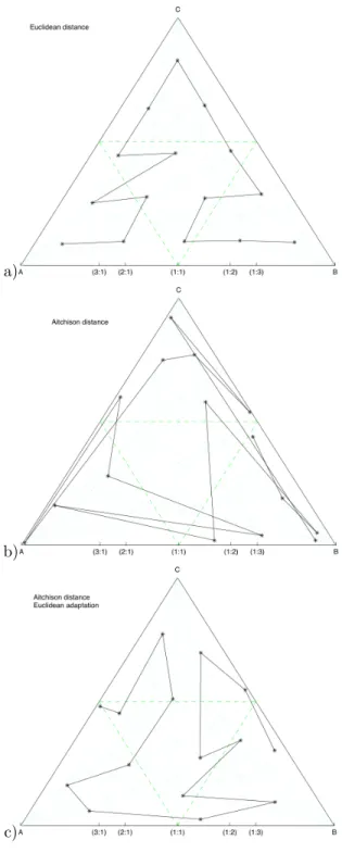
We tested three versions of the SOM algorithm with 4950 homogeneously (under Euclidean “eyes”) distributed input compositional data vectors on a three–part simplex. Initially, 15 model compo-sitional vectors were randomly generated. The characteristics of the three algorithms are:
1. SOM using Euclidean distance (Equation 1) to find the BMU and the adaptative function using the usual vectorial sum and scalar multiplication forRn
2. SOM using Aitchison distance (Equation 3) to find the BMU and the adaptative function using perturbation and powering (Equation 5)
3. SOM using Aitchison distance (Equation 3) to find the BMU and the adaptative function using the usual vectorial sum and scalar multiplication forRn
4.2
Example 2: Data set Hongite 4
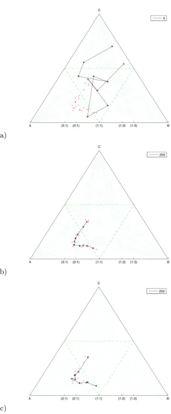
We then tested the 25 samples data set Hongite 4 from a three-parts simplex (Aitchison 1986) using two versions of the algorithm; 10 model compositional vectors were randomly generated:
1. SOM using Euclidean distance (Equation 1) to find the BMU and the adaptative function using the usual vectorial sum and scalar multiplication forRn.
2. SOM using Aitchison distance (Equation 3) to find the BMU and the adaptative function using perturbation and powering (Equation 5).
The results, after 250 iterations are presented in Figure 2.
4.3
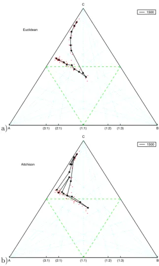
Example 3: two “compositional” straight lines
We tested two Aitchison’s straight lines in the simplex with additional random error. They, for example, represent two different evolutions of a volcanic sequence, from a original (source) com-position. In this example, 75 input samples were used (50 pertaining to one line and 25 to the other), and the duration of the training algorithm was 20 times the number of samples (i.e. 1500 iterations). The results are presented in Figure 3.
4.4
Example 4: AFM calc-alkaline trend from lavas of Hualca–Hualca
volcanic group, S. Per´
u
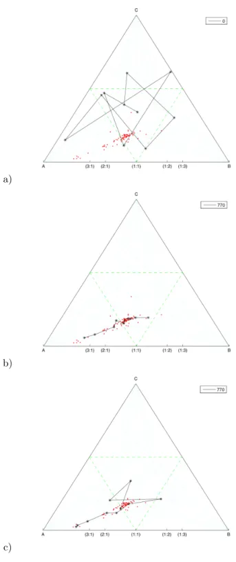
We tested a real data set of 77 calc-alkaline volcanic product from Hualca–Hualca volcanic group, southern Per´u (Klinck, Ellison, and Hawkins 1986) plotted in the AFM diagram, a three–part simplex designed for chemical classification (Irvine and Baragar 1971). We use two versions of the algorithm and 10 model compositional vectors randomly generated:
1. SOM using Euclidean distance (Equation 1) to find the BMU and the adaptative function using the usual vectorial sum and scalar multiplication forRn.
2. SOM using Aitchison distance (Equation 3) to find the BMU and the adaptative function using perturbation and powering (Equation 5).
The results, after 770 iterations are presented in Figure 4:
4.5
Example 5: AFM calc-alkaline trend from lavas of Hualca–Hualca
volcanic group, S. Per´
u, using all major elements.
Using the same data-set of the previous example, the algorithms were applied to the whole chemical analysis of the samples (10 major elements). Then, the plot AFM was obtained projecting the data and the model vectors in the three–part simplex using Irvine and Baragar (1971) projection. The duration of the training algorithm was 20 times the number of samples and the initial learning rate was set to 0.4. The results are presented in Figure 5.
5
Discussion and Conclusions
Results from the first example are particularly illustrative of the main predicament already exposed. It is indeed clear that the “homogeneously distributed” input vectors of the example are, under Aichison geometry, not distributed in that way, since the distances tend to infinity towards the “sides” of the ternary, thus expanding the distances between the input vectors when farther from the centre of the three–parts simplex (~0 = [0.330.330.33]); it is under and Euclidean approach that the input vectors appear homogeneously distributed, since the Euclidean distance between one and another adjacent is constant. The example clearly shows that the model vectors adapt better to the input vectors under Euclidean conditions since the ternary diagram represent a sort of a small cluster inRn therefore it is comparatively easy to position them in the proximity of the
input samples during the rough training. On the other hand, under the Aitchison geometry, the boundaries of the ternary are in the infinite, meaning that the data set is distributed in a non– homogeneous way in the whole space, with higher density of points in the centre than in the regions close to the boundaries of the diagram, suggesting that the rough training defined in this work is not adequate to position the neurons in the whole space. On the other hand, “well–behaved” scenarios like the real data set or the Hongite 4 example, the Aitchison’s “straight lines”, or the real volcanic samples, render more similar results under both approaches, but the Euclidean approach seems to converge faster and better to a well developed SOM, in which the connection between model vectors don’t cut themselves.
References
Aitchison, J. (1986).The Statistical Analysis of Compositional Data. Monographs on Statistics and Applied Probability. London: Chapman and Hall.
Aitchison, J., C. Barcel´o–Vidal, J. Mart´ın–Fern´andez, and V. Pawlowsky–Glahn (2000). Logratio analysis and compositional distance.Mathematical Geology 32(3), 271–275.
Egozcue, J. and V. Pawlowsky-Glahn (2006). Simplicial geometry for compositional data. In A. Buccianti, M.-F. G., and V. Pawlowsky-Glahn (Eds.), Compositional Data Analysis in the Geosciences, pp. 145–159. Geological Society, London, Special Publications, 264. Hertz, J., R. Palmer, and K. A.S. (1990). Introduction to the theory of neural computation.
Perseus Books.
Irvine, T. and W. Baragar (1971). A guide to the chemical classification of the common volcanic rocks.Canadian Journal of Earth Sciences 8, 523–545.
Klinck, B., R. Ellison, and M. Hawkins (1986). The geology of the cordilolera occidental and altiplano west of lake titicaca, southern per´u. Open file Report 353, British Geological Survey. Kohonen, T. (1997).Self–Organizing Maps (2 ed.), Volume 30 ofSeries in Information Sciences.
Appendix. Some relevant proofs
Proof 1: After adaptation the model vector is closer to the input vector,
no matter the geometry
In other terms, the BMU at iterationtshould be closer to the input vector after being updated, i.e: d(xj, wj(t+ 1))≤d(xj, wj(t))∀t (11)
in which the metricd(x, y) should be compatible with the operators defined for the space and also induce an inner product:
[d(x, y)]2=< x, x >−2< x, y >+< y, y > (12) in which< x, y >is the inner product ofxandy. Becaused(x, y)≥0 Equation 11 can be written as:
[d(xj, wj(t+ 1))]2≤[d(xj, wj(t))]2 (13)
Combining Equation 12 with Equation 13, Equation 11 is equivalent to:
< xj, xj >−2< xj, wj(t+1)>+< wj(t+1), wj(t+1)>≤< xj, xj>−2< xj, wj(t)>+< wj(t), wj(t)>
(14) or equivalently:
−2< xj, wj(t+ 1)>+< wj(t+ 1), wj(t+ 1)>≤ −2< xj, wj(t)>+< wj(t), wj(t)> (15)
Replacing wj(t+ 1) in terms of a generic adaptative function (Equation 5) and applying the
general properties of the inner product, in particular: < x⊕y, z >=< x, z > + < y, z > and < αx, y >=α < x, y >it can be shown that Equation 13 is equivalent to:
(α2−2α)[d(xj, wj(t)]2≤0 (16)
which is true when 0< α(t)≤1 since [d(xj, wj(t)]2 ≥0. Now, by definition (see section on the
Best matching unit and the adaptation function) the generic function 0< α(t)≤1 q.e.d.
Proof 2: Euclidean adaptation keeps compositional model vectors,
com-positional
The proof is straightforward: let bewj∈S the BMU neuron andx∈S the input vector. Because
both are compositionalP
iwij=kandPixi=kin which k is the closure constant of the simplex
S. Kohonen’s adaptative function has the following general Euclidean form:
wj(t+ 1) =wj(t) +α[x−wj(t)] (17)
we have to prove thatwj(t+ 1)∈S, which is equivalent to prove that Piwij(t+ 1) =k. From
Eq. 17: X i wij(t+ 1) = X i wij(t) +α[xi−wij(t)] (18)
using simply summing properties:
X i wij(t+ 1) = X i wij(t) +α[ X i xi− X i wij(t)] (19) hence: X i wij(t+ 1) =k+α[k−k] =k (20)
a)
b)
c)
Figure1: Results of the SOM representation of a compositional data set uniformly distributed in the Simplex (4950 samples). It was performed using a) Euclidean distance and adaptation, b) Aitchison distance and adaptation, and c) Aitchison distance and Euclidean adaptation. All the parameters were kept equal in each case.
a)
b)
c)
Figure 2: Results of the SOM representation of the data set Hongite 4 in a three–part simplex (25 samples). a) Initial conditions, b) Euclidean distance and adaptation, and c) Aitchison distance and adaptation. All the parameters were kept equal in each case.
a)A (3:1) (2:1) (1:1) (1:2) (1:3) B C 1500 Euclidean b)A (3:1) (2:1) (1:1) (1:2) (1:3) B C 1500 Aitchison
Figure3: Results of the SOM representation for two Aitchison’s straight lines with random error. a) Euclidean distance and adaptation, and b) Aitchison distance and adaptation.
a)
b)
c)
Figure4: Results of the SOM representation of a calc–alkaline data set (77 samples) from Hualca–Hualca volcano southern Peru in the three–part simplex AFM diagram. a) Initial conditions, b) Euclidean distance and adaptation, and c) Aitchison distance and adaptation. All the parameters were kept equal in each case.
a)A (3:1) (2:1) (1:1) (1:2) (1:3) B C 0 Euclidean b)A (3:1) (2:1) (1:1) (1:2) (1:3) B C 0 Aitchison
Figure5: Results of the SOM representation of a calc–alkaline data set (77 samples) from Hualca–Hualca volcano southern Peru, calculated using the whole data-set and then projected in the three–part simplex AFM diagram. a) Euclidean distance and adaptation, and b) Aitchison distance and adaptation.