Modal Analysis of Weak Networks with the Integration of Wind Power

(1)

June 2008

Olav B Fosso, ELKRAFT

Master of Science in Energy and Environment

Submission date:

Supervisor:

Norwegian University of Science and Technology

Department of Electrical Power Engineering

Modal Analysis of Weak Networks with

the Integration of Wind Power

(2)

(3)

Problem Description

When increasing the integration of wind power, both the steady-state and the dynamic behaviour of the system are affected. Since wind power facilities often are located in areas with weak networks (low short circuit capacity), disconnection of generators leading to power outage might occur at small disturbances. New requirements are therefore introduced, demanding that the facilities are not disconnected at a defined type of disturbance with specified time duration (fault-ride-through).

The main objective is the focus on how different types of wind power facilities affect a network’s dynamic stability when exposed to small disturbances. This implies dynamic simulations for typical wind series and systematically use of linear analysis (eigenvalues, sensitivities, etc) in order to identify critical variables.

Analyses shall be carried out for wind power facilities based on both constant speed wind turbines and variable speed wind turbines. Dynamic models of SVC and traditional condenser batteries can be used if found necessary.

The following activities shall be included:

• Describe the current models for wind power turbines and demonstrate an understanding of the different models and how these interact.

• Identify crucial parameter values and evaluate the optimal placement of critical eigenvalues.

• Demonstrate how the linear analysing technique can be used to find the interaction between components in a dynamic system and by that contribute to optimal system behaviour. • Analysis of a small-scale network with a combination of different production sources. Obtain results which are illustrative.

The analyses shall in general be based on the simulation software SIMPOW. MATLAB can also be used to evaluate the results.

The Master Thesis is a continuance of a project during the fall of 2007. Assignment given: 17. January 2008

(4)

(5)

Abstract

In this master thesis the theory and practical use of modal analysis is explained, giving an introduction to the possibilities of modal analysis. The master thesis starts with a look at wind power and the design of a modern wind turbine. Two models, one for constant wind speed wind turbines and one for variable speed wind turbines, are presented. An example shows how modal analysis can be utilized to evaluate a network's dynamic stability. Simulations are performed on a two-area network where dierent wind power models are tested and compared.

A two-mass model is used to model a constant wind turbine. The model consists of an asynchronous generator, a turbine, and a low speed shaft with a tensional stiness. The model representing the variable speed wind turbine is based on a DFIG model included in the simulation software.

The two-area network consists of two areas connected together through a long line be-tween Bus 5 and Bus 6. Area 1 has two production sources, one placed in Bus 1 and one placed in Bus 2. The second area represents a large network modelled as a very large synchronous generator with a high inertia.

The calculations have showed how modal analysis can be used to evaluate a system by using linearized dierential equations and how the systems robustness against small disturbances can be altered by changing the systems parameters.

Simulations have veried that a two-mass model must be used when modelling a constant speed wind turbine. The inertia of the turbine will greatly inuence the model's behaviour and must therefore be included in the model. Eigenvalues analysis performed during dierent wind speeds have documented that wind power will not become less stable towards small disturbances when operated at low wind speed conditions.

(6)

(7)

Preface

This master thesis has been written at the Department of Electric Power Engineering at the Norwegian University of Science and Technology during the spring of 2008. The thesis represents the end of my two years international master study.

Wind power facilities are often located in areas with weak networks, disconnection of generators leading to power outage for small disturbances. This thesis deals with the possibilities of applying modal analysis to a weak network with the integration of wind power.

The master thesis is written in the text formatting system LA_{TEX, calculations are done}

in MATLAB and simulations have been executed in SIMPOW.

I would like to thank my subject teacher and supervisor Prof. Olav Bjarte Fosso for his valuable guidance and help. I would also like to thank Ph.D. student Jarle Eek and Trond Toftevaag at SINTEF Energiforsking AS for important help with the simulations.

Trondheim, June 2008

Asbjørn Benjamin Hovd

(8)

(9)

List of Figures

2.1 Traditional "Dutch" windmill [1] . . . 3

2.2 Components of a wind turbine . . . 4

2.3 European wind map [2] . . . 5

2.4 Installed wind power in Europe [3] . . . 6

3.1 General model of a wind turbine [4] . . . 7

3.2 Constant speed wind turbine with squirrel cage induction generator [5] . . 8

3.3 General SCIG model [5] . . . 9

3.4 Two mass model [6] . . . 9

3.5 Variable speed wind turbines. . . 10

3.6 General variable speed wind turbine model [5] . . . 10

3.7 Block diagram of DFIG model [7] . . . 11

3.8 The speed control [7] . . . 11

3.9 The pitch control [7] . . . 12

3.10 The crow-bar resistor control [7] . . . 13

3.11 The AC bus control [7] . . . 13

4.1 Inter-area oscillation [8] . . . 17

4.2 Inter-area and local-area oscillations [8] . . . 17

5.1 Dynamic system [9] . . . 20

5.2 An Eigenvalue in the complex plane and the time plane [9] . . . 23

5.3 Eigenvalues in complex plane and with damping ratio . . . 24

5.4 Block diagram representation [10] . . . 26

6.1 SMIB system [11] . . . 29

6.2 Equivalent circuit in the sub-transient state . . . 29

6.3 Equivalent circuit of synchronous generator [12] . . . 30

6.4 Three bus example . . . 35

6.5 Dierent inertia values . . . 38

6.6 Dierent line reactance values . . . 39

7.1 2 Bus system, DFIG and innite bus . . . 41

7.2 The AC bus control [7] . . . 42

7.3 Change of eigenvalue 4,5 . . . 43

7.4 Three phase fault at Bus 1 . . . 43

7.5 Correlation between wind speed, blade angle and produced power . . . . 44

7.6 Power curves for dierent wind speeds . . . 44

7.7 2 Bus system, SCIG and innite bus . . . 45

7.8 Sensitivity overview for eigenvalue 3,4 and 6,7 . . . 45

(14)

7.9 Change of Torsional stiness, eigenvalue 3,4 and 6,7 . . . 46

7.10 Oscillations after fault . . . 46

7.11 Speed increase when torque is increased . . . 47

7.12 Two area network . . . 48

7.13 Mode shape for inter-area mode . . . 51

7.14 Dominant participation factors for inter-area mode . . . 52

7.15 Speed response for conguration A1 . . . 52

7.18 Speed response for conguration B2 . . . 54

7.24 Mode shape for local-area mode . . . 61

7.25 Dominant participation factors for inter-area mode 8,9 . . . 61

7.26 Speed response for conguration E2 . . . 62

7.27 Mode shapes inter-area mode, all main congurations . . . 63

7.28 G1 Speed response for conguration A1, B2 and E2 . . . 64

7.29 Speed response for Synchronous generator and SCIG . . . 64

A.1 Three bus example . . . 72

A.2 The MATLAB program . . . 74

A.3 Load ow from SIMPOW . . . 78

A.4 Eigenvalues in SIMPOW when changing inertia from 1 to 10 . . . 78

C.1 All eigenvalues before and after improvement . . . 86

C.2 Eigenvalues with changed KP and KS . . . 86

C.3 Eigenvalues at dierent wind speeds. . . 87

C.4 Eigenvalues, constant power . . . 87

C.5 Eigenvalues with dierent torque . . . 88

C.6 Eigenvalues A : Synchronous generator. . . 92

C.7 Eigenvalues, B : Asynchronous generator. . . 93

C.8 Eigenvalues C : Static production. . . 94

C.9 Eigenvalues D : DFIG. . . 95

C.10 Eigenvalues E : SCIG. . . 96

(15)

List of Tables

6.1 Dierent line reactance values . . . 39

7.1 Eigenvalues for DFIG . . . 42

7.2 Sensitivity overview eigenvalue 4 . . . 42

7.3 Eigenvalues . . . 43

7.4 Eigenvalues with constant power . . . 45

7.5 Eigenvalues with changed torque . . . 47

7.6 Congurations on Bus 1 (NA=not available) . . . 49

7.7 Eigenvalues, A1 : Synchronous generator with VC . . . 50

7.8 Eigenvalues, A2 : Synchronous generator and SVC . . . 50

7.9 Eigenvalues, A3 : Synchronous generator and SCRC . . . 50

7.10 Inter-area and local-area eigenvalues . . . 51

7.11 Eigenvalues, B2 : Asynchronous generator and SVC . . . 52

7.12 Eigenvalues, B3 : Asynchronous generator and SCRC . . . 53

7.14 Eigenvalues, C2 : Static production and SVC . . . 55

7.15 Eigenvalues, C3 : Static production and SCRC . . . 55

7.17 Eigenvalues, D1 : DFIG with VC . . . 57

7.18 Eigenvalues, D2 : DFIG and SVC . . . 57

7.19 Eigenvalues, D3 : DFIG and SCRC . . . 57

7.21 Eigenvalues, E2: SCIG and SVC . . . 59

7.22 Eigenvalues, E3 : SCIG and SCRC . . . 59

7.24 Eigenvalue 8,9 . . . 60

A.1 Parameters for Synchronous Generator . . . 72

A.2 Predened and calculated values . . . 73

A.3 Line data . . . 73

B.1 Original -and aggregated values for DFIG . . . 81

B.2 Parameters for SCIG from [4] and [7] . . . 83

C.1 Bus data . . . 89

C.2 Line data . . . 89

C.3 Transformer data . . . 89

C.4 Peak to Peak values . . . 93

C.5 Damping . . . 93

(16)

(17)

Nomenclature

Scalars

β Turbine blade angle

∆ωr per unit speed deviation

∆W Speed deviation δ rotor angle

Λ Tip speed ratio

λ Eigenvalue

Ω Rotational speed of wind turbine

ω Imaginary part of the eigenvalue ∂ Partial derivative

ρair Density of wind

σ Real part of the eigenvalue ζ Damping ratio

Arotor Areal of rotor

Cp Turbine eciency

E Steady state internal emf f Frequency

H Mechanical inertia I Current

J Inertia

K Speed calculation coecient KD Generator damping power

Ks Synchronizing torque coecient

ks Torsional Spring Constant

Pord Power order

(18)

Pwind Power extracted from wind

P eg Optimal generated power Qord Reactive power order

R Resistance

Rblade Length rotor blades

S Apparent power Te Electrical Torque

Tm Mechanical Torque

V Voltage

Vac,ref node reference voltage

vwind Wind speed

Wref Rotational speed reference

X Reactance Z Impedance Pe Power produced

T_d,,T_d,, short-circuit d-axis transient and sub-transient time constants Te Electrical Torque

Tq,,Tq,, short-circuit q-axis transient and sub-transient time constants

T_d,₀,T_d,,₀ open-circuit d-axis transient and sub-transient time constants T_q,₀,T_q,,₀ open-circuit d-axis transient and sub-transient time constants Xd,X_d,,X_d,, d-axis synchronous, transient and sub-transient reactance

Xq,Xq,,Xq,, q-axis synchronous, transient and sub-transient reactance

Vectors and Matrices u Input vector x State vector y Output Vector

.

x State vector derivatives A System matrix B Control matrix B Feed-forward matrix C Output matrix I Identity matrix P Participation matrix xiv

(19)

XL Left eigenvector

XR Right eigenvector

Units

m meters

m/s Meter per second p.u. Per unit

rpm Revolutions per minute

AC Alternate Current MVA Megavoltampere MW Megawatt Hz Hertz Abbreviations

DDSG Direct Drive Synchronous Generator DFIG Doubly Fed Induction Generator HVDC High Voltage Direct Current

SCRC Static Constant Reactive Compensation SVC Static Var Control

VC Voltage Control emf Electro-motive force

SCIG Squirrel Cage Induction Generator

(20)

(21)

Chapter 1

Introduction

1.1 Motivation

Norway has with its long coastline and good wind conditions the possibility to extend its current wind utilization greatly. Several wind farms are therefore planned which will considerably increase the amount of wind power in the Norwegian power system. Since wind power must be placed along the coast or at other locations where the wind conditions are good, most wind farms will be located far away from the load centres and in relatively weak networks with low short circuit power.

Wind power is an uctuating power source where the amount of produced power varies with the wind speed power. Combined with the fact that wind power technology dif-fers from the technology used in the synchronous water power plants dominating the Norwegian power systems today, leads to new and demanding challenges.

1.2 Background

The recent years' considerable growth of installed wind power has led to considerable research concerning the performance of wind turbines towards power system dynamics, transient stability and their response to short circuits. Small small signal stability on the other hand has so far received much less attention. Small signal stability is as described in chapter 4 the systems ability to reach a steady state condition after a small disturbance. This is mainly a problem due to insucient damping of electromechanical modes, which are related to power oscillations occurring in the rotor of electrical machines [13].

1.3 Research Objective

The scope of this master thesis is to see how dierent types of wind power facilities aect a network's dynamic stability when exposed to small disturbances. This includes dynamic simulations for typical wind series and a systematically use of linear analysis (eigenvalues, sensitivities, etc) in order to identify critical variables.

Description of the currents models for wind power models shall be presented and a demonstration on how linear analysing techniques can be used to nd the interaction between components in a dynamic system and by that contribute to optimal system behaviour are to be carried out.

(22)

2 CHAPTER 1. INTRODUCTION A small SMIB network and a network with an sucient degree of freedom are to be used to simulate and evaluate the dierent wind farm representations.

1.4 Content of the Thesis

The master thesis can in general be divided into three main parts:

Chapter 2-5. These chapters contains the theory part of the thesis. Chapter 2 present wind power in a historical perspective and explains the design of a modern wind turbine, while chapter 3 looks closer into a general wind turbine model and presents the models used in the simulations. The theory behind small signal stability and the mathematical expressions are presented in chapter 4-5.

Chapter 6. This chapter uses a small network with an synchronous generator to demon-strate how linear analysis can be applied on a power system.

Chapter 7. Two SMIB systems, one with a constant speed wind turbine and one with a variable speed wind turbine is simulated and several models are tested on a two area network.

(23)

Chapter 2

Wind Power

This chapter gives a brief introduction to the history and development of wind power. The design of a modern wind turbine is explained and a market overview for Europe is presented.

2.1 Historical Perspective

Wind power have been used to pump water, grind corn and cross oceans for thousands of years, and early examples of wind powered machines were used in Persia as early as 200 BC. The rst known practical windmills were probably built in Sistan, Afghanistan around the seventh century. These windmills were vertical axles with rectangle shaped blades and were used to grind corn and pump water. Windmills for grinding corns were also used in a large scale in Europe and by the late nineteenth century more than 100.000 "Dutch" windmills were in use [1].

Figure 2.1: Traditional "Dutch" windmill [1]

In 1887 the rst known electrical wind turbine was built in Scotland and there were in 1908 around 70 wind-driven electric generators ranging from 5 kW to 25 kW. Some larger mills were built later on, but due to large scale grid electrication projects all interest for windmills halted in the late 1930's [14].

(24)

4 CHAPTER 2. WIND POWER

2.2 Modern Wind Turbines

A wind turbine is by denition a machine that converts wind power into electrical power. Most turbines in use today are of a fairly large size, ranging from 500 Kw and up 4 MW. Most new turbines are also, in order to better utilize the space, constructed in clusters, more commonly known as wind farms.

Modern wind turbines uses the aerodynamic force of lift and converts it into a mechanical torque on a rotating shaft which is transformed into electricity by a generator. The amount of power from a wind turbine highly depends on the wind speed and since the wind is always changing, wind turbines must be treated as uctuating and non-dispatchable energy sources. Power systems with installed wind power generation must therefore be designed with this factor taken into consideration.

Formula 2.1 shows the produced power as a function of wind speed, wind density and the area covered by the blades. The formula indicate that the produced power increases with the cubic of the wind speed.

Pwind=

1

2CpρairArotorv

3

wind (2.1)

When the wind speed is low there is very little energy in the wind. A wind turbine will therefore not start to produce power until the wind reaches a predened cut-in speed, normally around 3-5 m/s. As the speed increases and reaches nominal speed, around 12-15 m/s, the power taken out from the wind must be reduced or the wind turbine can be exposed to large forces that eventually will damage the wind turbine.

All commercially available wind turbines today are based on the horizontal axis design and aligned with the wind. The principal subsystem of a modern wind turbine is shown in gure 2.2:

(25)

2.3. WIND RESOURCES 5 An in-depth explanation of the various components in a wind turbine can be found in the book "Wind energy Explained, Theory, Design and application" [15]

2.3 Wind Resources

Small changes in wind will drastically change the amount of power produced from a wind turbine. It is therefore vital to investigate the wind resources in a area before planning of building a wind farm.

Figure 2.3: European wind map [2]

Figure 2.3 shows the onshore European wind resources at a height of 50 metres. Darker colour indicates stronger wind and it is clear that the United Kingdom and especially the coast of Norway have an exceptional potential for wind power.

2.4 Market overview

Figure 2.4 shows the amount of installed wind power in Europe. Around two-thirds of all the installed capacity is located in Germany and Spain, countries that according to the wind atlas experiences small amounts of wind, while Norway with its huge potential only have 0.005 percentage of the installed capacity in Europe. This implicates that

(26)

6 CHAPTER 2. WIND POWER even though a large amount of wind parks are planned to be erected in Norway, giving an considerable increased installed capacity, there is still potential for much more wind power in the years to come [16].

(27)

Chapter 3

Wind Turbine Modelling

This chapter explains the importance of using a model intended for the required appli-cation. A general model is explained and models for constant speed wind turbines and variable speed wind turbines are presented

3.1 Introduction

A typical power system consists of many components such as overhead lines, underground cables, transformers, generators and loads. Since most components can be described by dierential equations, a large system would need several thousands of dierential equations to describe the system. It is therefore necessary to take into account a model's intended application and ensure that the model gives reliable results while not being too complex.

Since the scope of this project is to look into linear stability, it is only necessary to study phenomena occurring in the frequency range of 0.1 Hz and up to 10 Hz. Phenomena with a frequency above or below this range can therefore be neglected because they most likely do not aect the investigated phenomena [5].

3.2 General Model

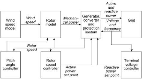
Figure 3.1: General model of a wind turbine [4]

The basic working principle of all wind turbines is, as described in chapter 2, basically the same. It is therefore possible to use a general model of a wind turbine in order to visualize the working principle. The model in gure 3.1 is one example on how such

(28)

8 CHAPTER 3. WIND TURBINE MODELLING a model could look like. The wind speed model simulates the wind passing the wind turbine, while the aerodynamic model translates this wind into mechanical power which goes trough the shaft and other mechanical components and into the generator. A more detailed description of the dierent parts are given in the specialisation project [17] It is how ever not always sucient to use a general model to describe all wind turbines and it is often common to divide dierent wind turbine technologies into two dierent types:

• Constant speed wind turbines • Variable speed wind turbines

The constant speed turbine uses a generator directly coupled to the network. This means that the speed of the generator will follow the system frequency and the speed variations will due to the slip in the generator only be around 1 or 2 percents. A variable speed turbine's frequency is on the other hand decoupled from the electrical grid. This allows for variable speed operations since the electrical stator and rotor frequency can be matched independently of the mechanical rotor speed [5]. This dierences in working principles necessitate the use of two dierent model when simulating wind power.

3.3 Constant Speed Wind Turbines

Figure 3.2: Constant speed wind turbine with squirrel cage induction generator [5]

Most constant-speed wind turbines in use today are based on the squirrel-cage induction generator, hereby referred to as SCIG. The Generator is directly coupled to the grid and since the slip and the rotor speed variations are so small the SCIG is described as xed speed.

SCIG wind turbines normally uses stall control to limit the power from the wind. This means that the blades are constructed in such a way that they start stalling when the wind reaches a predened value, thereby reducing the lift.

(29)

3.3. CONSTANT SPEED WIND TURBINES 9

Figure 3.3: General SCIG model [5]

3.3.1 Constant Speed Wind Turbine Modelling

Figure 3.3 shows the general structure of a SCIG wind turbine as presented by [5]. This model includes all the parts necessary to perform a complete analysis of the turbine, including the power system model.

Since the main objective of this thesis is to perform small signal stability studies, which must be performed when the system is at steady state, it is not critical to include the "Wind speed" block. This block is therefore not included in the simulated model. The "Rotor model" is modelled using a turbine where an arbitrary time function f(t) is multiplied with the initial value of the mechanical torqueT m0[7]. Since the time function

is given as a table it is also possible in a simplied way to simulate wind speeds by changing the amount of torque during the simulation.

Figure 3.4: Two mass model [6]

Figure 3.4 shows the drive train of a wind turbine. Since the resonance frequency of the high speed shaft and the gearbox are much higher than the bandwidth of interest, only the spring constant of the low speed shaft needs to be modelled [5]. The drive train can therefore be modelled using a two-mass model where the rotor is modelled with an inertia Jwtr and generator inertia Jgen is implemented in the generator. The torsional

spring constant of of the low speed shaft is modelled by the stiness constantks.

The squirrel cage induction generator is modeled according to the parameters used in [4]. They represent the values of a single wind turbine in the wind farm Hagesholm in Eastern Denmark. These values are changed into PU values and aggregated in order to simulate a large wind farm.

A full list of all the wind turbine parameters, calculations for implementation into SIM-POW and the SIMSIM-POW simulation les can be found in appendix B.2

(30)

10 CHAPTER 3. WIND TURBINE MODELLING

3.4 Variable Speed Wind Turbines

(a) DFIG (b) DDSG

Figure 3.5: Variable speed wind turbines. From left: doubly fed induction generator and direct drive synchronous generator [5]

Figure 3.5 illustrates the two main types of variable speed wind turbines on the mar-ket. They both use power electronics to decouple the mechanical rotor speed from the electrical frequency, enabling them to change the rotor speed independently of the grid frequency. The DFIG uses a back-to-back converter feeding the three phase rotor wind-ing, while the DDSG uses a full scale converter completely decoupling the generator from the grid [5].

Both solutions have a several advantages and drawbacks. In the DFIG only 30 % of the power passes through the converter while the converter in the DDSG must be of full scale. The DDSG does on the other hand not need a gear box but must use a large, heavy and complex ring generator. A more in-depth explanation on the dierences between DFIG and DDSG can be found in [15].

3.4.1 Variable Speed Wind Turbine Modelling

Figure 3.6: General variable speed wind turbine model [5]

A general model for a variable speed wind turbine as presented in [5] is shown in gure 3.6. Simulations performed on both DFIG and DDSG in [5] revealed that there is a high degree of similarity in the simulation results for these technologies. This occurs since only the rotor speed controller and the pitch angle controller governs the frequency

(31)

3.4. VARIABLE SPEED WIND TURBINES 11 bandwidth of interest. Since these controllers often are similar in both the DFIG and the DDSG, it can be concluded that both types can be represented by the same model in power system dynamics simulations [5].

SIMPOW includes a model of a DFIG wind turbine designed for system analysis of power ow and electromechanical transients. This models have all the components necessary to perform a full analysis of a variable wind turbine and has therefore been used in this thesis to simulate a variable speed wind turbine.

The model in SIMPOW consists of six modules as shown in gure 3.7. The explanations on this model is mainly from [7] and [18].

Figure 3.7: Block diagram of DFIG model [7]

The asynchronous machine model consists of a wound rotor induction generator. The rotor uses slip rings for the external rotor circuit where an simplied loss-less frequency converter modelled as a voltage source is placed. The frequency converter transfers during negative slip, real power from the rotor to the grid and real power from the grid to rotor during positive slip.

The inertia of the DFIG wind turbine is modelled as one rotating mass placed in the generator. This can be done since the controllers of the turbine will minimize the eects of the turbine shaft and it is therefore not necessary to use a two mass model [5].

Figure 3.8: The speed control [7]

The speed control is used to control the rotational speed and generated real power. A speed reference (Wref) is found by using the real power generation in the formula:

(32)

12 CHAPTER 3. WIND TURBINE MODELLING

Wref =A2Peg2 +A1Peg+A0 (3.1)

WhereA0, A1 and A2 are coecients dened in such a way that optimal wind power is

captured (see appendix B.1).

When the optimal speed reference is obtained, the dierence between the reference and real speed is calculated and sent through a PI-controller and multiplied with the real speed. This gives the Power order Pord, which is sent trough a lter and back to the

generator. The power order now ensures that the generator's rotational speed is optimal compared to the wind speed. The control range of the speed is about+/−0.25−0.30pu.

Figure 3.9: The pitch control [7]

All variable wind turbines uses a form of pitch control in order to reduce the force of power obtained from the wind. This ensures that the wind turbine can be safely operated even though the wind speed exceeds the wind needed to obtain rated generator power. Figure 7.5 in section 7.1.2 shows how the wind turbine starts to pitch the blades as the wind speed increases in order to keep the power output constant.

The pitch control uses the power order (Pord) obtained from the speed control and

com-pares it with the speed deviation (∆W) which is also from the speed control. The sum

of these outputs gives the optimum blade angle for the turbine. The blade angle (β) is

then ltered to ensure that it does not exceed the maximum or minimum blade angle of the wind turbine.

If a fault appears on the line resulting in a large voltage change on the wind turbine terminals, it is vital that the frequency converter is quickly disconnected to prevent it from failure. If such a fault should appear the Crow-bar resistor control will measure the node voltage and if the voltage is found to be outside the boundaries, the frequency converter will be disconnected and the external rotor circuit will be connected to a crow-bar resistor.

(33)

3.4. VARIABLE SPEED WIND TURBINES 13

Figure 3.10: The crow-bar resistor control [7]

Figure 3.11: The AC bus control [7]

the amount of reactive power produced or consumed by the generator. The AC voltage control regulator does this by measuring the node voltage and comparing it with a refer-ence voltage (Vac,ref = 1.0pu). If the measured voltage is below or above the reference,

a reactive power order (Qord) is sent to the generator, making it produce or consume

reactive power

SIMPOW uses as default a DFIG with a rated size ofSn= 2.05M V A. The model used

in the simulation is much larger and it is important to ensure that the ratio between nominal power, blade length and turbine speed remains the same. The aggregation of the DFIG wind turbine and the complete SIMPOW les can be found in appendix B.1.

(34)

(35)

Chapter 4

Power Oscillations

This chapter explains the nature of power oscillations, why they occur, and how they can be mitigated. A quick look at wind power versus power system oscillations is presented.

4.1 Introduction

Power systems contain many modes of oscillation due to a variety of interactions among components. Most of these oscillations originate from generators swinging relative to one another. The modes involving these masses most often occur in the frequency range of 0.1 to 2 Hz [19] and can cause the oscillation of other power system variables (bus, voltages, bus frequency, transmission lines, active and reactive power, etc).

Oscillations in the 1 to 2 Hz range are most often a result of a single generator or a group of generators oscillating against the rest of the system. These oscillations are most often referred to as "local-area oscillations" . Oscillations occuring in the 0.1 to 0.5 Hz range are referred to as "inter-area oscillations", and involve groups of generators in one area oscillating against generators in another area. These oscillations are particularly troublesome and can in some cases constrain system operation.

Power system oscillations can be stimulated trough a number of mechanisms. Oscillations may be triggered trough a disturbance on the power system, or by crossing some steady-state stability boundaries. Undamped oscillations can, once started, grow in magnitude over a few seconds and lead to the loss of synchronism, loss of part or losses of all electrical network. Network outage can also occur if the oscillations are strong and persistent enough to cause uncoordinated automatic disconnection of key generators or loads.

The two most common reasons for instability is:

• Steady increase in generator rotor angle due to lack of synchronizing torque. • Rotor oscillations of increasing amplitude due to lack of sucient damping torque.

Small signal stability or steady state stability is the systems ability to maintain synchro-nism during small disturbances, or as given by IEEE [20]:

A power system is steady-state stable for a particular steady-state operating condition if, following any small disturbance, it reaches a steady-state oper-ating condition which is identical or close to the pre-disturbance operoper-ating condition. This is also known as Small Disturbance Stability of a Power Sys-tem

(36)

16 CHAPTER 4. POWER OSCILLATIONS The disturbances must be so small that the equations describing the dynamics of the power system can be linearized for the purpose of analysis. This is further explained in chapter 5.

4.2 Historical perspective

Oscillations between generators have appeared since the rst ac-generators where oper-ated in parallel. These oscillations where expected due to synchronous generators power vs. phase-angle curve gradient, forming an equivalent mass and spring system. Varying load of the generators would therefore continually trigger the oscillations.

Power system oscillations were for a long time not regarded as a problem and most an-alytical tools seemed to ignore damping entirely. This changed rather suddenly in the 1960's when an increasing number of networks, were interconnected, and more negative damping was introduced by the increasing use of high responsive generator voltage regu-lators. The increasing complexity of the power systems and tie-lines of limited capacity led to the reappearance of power system oscillations.

4.3 Types of Power System Oscillations

Power system oscillations can in general be divided into four types:

• Local plant mode oscillations • Inter-area mode oscillations • Torsional mode oscillations • Control mode oscillations

Local plant mode oscillations are the most common oscillations and are associated with the swinging of units at a generating station against the rest of the power system. These oscillations normally occur in the range of 1 to 2 Hz.

Inter-area mode oscillations are associated with the swinging of a group of machines in one part of the system against groups of machines in other parts of the system. They are caused by two or more groups of machines being interconnected by weak tie-lines. These oscillations normally occur in the range of 0.1 to 1 Hz and are normally the oscillations which present the greatest challenge.

Torsional mode oscillations comes from the turbine-generator rotational components and can lead to instability due to interactions with the generating units and prime mover control.

Control mode oscillations are associated with the control of generating units and other equipment and are normally caused by poorly tuned controls of excitation systems, prime movers, static var compensators and HVDC converters.

Figure 4.1 shows an inter-area oscillations between two areas. The generators in each area are in phase with each other and in anti-phase with the generators in the another area.

(37)

4.4. REASONS FOR POWER SYSTEM OSCILLATIONS 17

Figure 4.1: Inter-area oscillation [8]

(a) Inter-area (b) Local-area

Figure 4.2: Inter-area and local-area oscillations [8]

The left picture gure in 4.2 shows the same inter-area oscillation as in gure 4.1. The picture in the right side show a local-area oscillation where the two generators in area 1 are oscillating against each other

4.4 Reasons for Power System Oscillations

Power system oscillations are as previous mentioned, normally a result of the power vs. phase-angle characteristic in synchronous generators, but the damping can be improved or worsen by many dierent factors. When only a few generators are paralleled in a closely connected system, oscillations are damped by the generators damper windings and only small variations in system voltage can occur. The generators voltage regulators will therefore not participate in the activity, and increasing the regulators' response will not decrease the system damping, but only improve the transient stability.

If this system is now connected to a similar system by a tie-line with only a fraction of the system capacity, this would due to the tie-line's high impedance, greatly reduce the damper positive damping. The generators' terminal voltage will become more responsive to angular swings and cause the regulators to react, thereby producing negative damping.

(38)

18 CHAPTER 4. POWER OSCILLATIONS Tie-line oscillations are likely to occur, which can lead to transfer restriction on the tie-line.

4.5 Wind Power and Power System Oscillations

Since the mechanical parts of a synchronous machine have low damping of low oscillations the damping must come from other sources, such as the damper windings, the machine's controllers and other parts of the power system. But the very low frequency of the power system oscillations are hardly damped by the damper windings, thus leaving the controllers and the rest of the system as the main contributors to the damping of the rotor speed oscillations. Most wind turbines however, including the models used in this thesis, uses an asynchronous generator which in contrast to the synchronous generator does not show oscillatory behaviour since the generator have a correlation between rotor slip and electrical torque. The mechanical part is therefore of rst order and does not oscillate. The generator used in variable speed wind turbines such as the DFIG, is decoupled from the power system by power electronic converters. The generator does therefore not react to any oscillations in the power system as they are not transferred trough the converter [5].

(39)

Chapter 5

Modal Analysis

Modal analysis is a powerful and helpful tool in order to locate and mitigate power system oscillations. Modal analysis assumes a linearized model of the system in a state space form. This chapter explains the linearization of a system and presents the modal analysis methods used by most simulations software.

5.1 Introduction

Analyzing power system oscillations require a combination of analytical tools. Oscilla-tions are often observed in transient non-linear simulaOscilla-tions and a complete understanding of the system will therefore require programs both for linear analysis and for non-linear analysis.

Programs capable of analyzing power system oscillations have historically been, due to the mathematical nature of the techniques required, restricted to fairly small networks. The recent years development of mathematical tools for analyzing the oscillatory behaviour of power systems have led to a large number of commercially available tools, capable of both linear and non-linear simulations.

5.2 Modal Analysis

Modal analysis is used to nd the nature of the oscillations and it is a very useful tool to determine the characteristic modes of a system linearized around a specic operating point. By applying modal analysing to a power system it is possible to locate the devices participating in the oscillations and use this information to do the required action in order to solve the problem.

Models of power systems uses non-linear algebraic dierential equations to represent the components. When using modal analysis, these equations are linearized about an operat-ing point by the use of Taylor series expansion. This sections describes the mathematical methods used in power system modal analysis.

5.2.1 State-Space Model

A state-space model is in many ways just a dened way to write a system's dierential equations. The variables used in the state-space model amount to the system's state variables. The state variables of the dynamic system can be physical quantities such as

(40)

20 CHAPTER 5. MODAL ANALYSIS angle, speed or dierential equations describing the dynamics of the system. Together with the inputs to the system, the state variables give a complete description of the system behaviour.

Figure 5.1: Dynamic system [9]

Figure 5.1 shows a dynamic system with its input vector u, output vector y and the state vector x, containing the state variables of the dynamic system.

When given a non-linear continuous time dynamic system, one equation is used to de-termine the state of the system and another equation to dede-termine the output of the system.

The equation describing the state of the system will then have the form [21]:

. x=f(x, u) (5.1) x=      x1 x2 ... xn      u=      u1 u2 ... un      f =      f1 f2 ... fn      (5.2)

The equation describing the system's output will have the form:

y=g(x, u) (5.3) y=      y1 y2 ... ym      g=      g1 g2 ... gm      (5.4) 5.2.2 Linearization

Linearization is a useful tool when studying a systems behaviour around an operating point. Linear equations can be used to describe the new system, assuming that all deviations are small. The non-linear system can then be made into a linear system, since linear equations are sucient to describe the system.

Linearization methods can generally be classied into three groups [22]:

(41)

5.2. MODAL ANALYSIS 21

• Numerical linearization • Analytical linearization

System identication measures or simulates the response of non-linear systems to change of inputs. A suitable model is selected and parameter identication tech-niques are used to obtain parameters for the linear system. System identication methods are rarely used for linearization of power system components models. Numerical linearization measures the response of the system by calculating deviation

of state derivatives after a small change has been applied to the inputs and the states. This enables the calculation of the states space matrices by the use of dierence equations: Aij = ∆fi ∆xj = fi(xδu0)−fi(x0, u0) xδ,j−x0,j (5.5)

where subscriptδ is used for vector with changed jth and subscript δ, j is used for

the value of that specic component.

This method is widely used in power systems, such as PSS/E. It is quick and simple, but can only provide an approximation of the precise analytical solution. It is also necessary to repeat the linearization procedure each time the operating point changes.

Analytical linearization is based on analytical computation of system Jacobians. An-alytical linearization is very precise and when the operation point changes, new matrices are easily obtained by substituting the new operating points in the Jaco-bians.

The simulation software used in this thesis, SIMPOW, uses analytical linearization where all dierential equations are linearized by their analytical expressions [23]. The eigenvalues of matrix A is then solved using the QR-method, which is further explained in section 5.3.1.

5.2.3 Principles of Linearization

By applying a small disturbance in both the state vector and the input vector the new state of the system presented in section 5.2.1 can be written as:

.

x=x.0+ ∆

.

x=f[(x0+ ∆x),(u0+ ∆u)] (5.6)

Formula 5.1 can now, by using Taylor series expansion, and neglecting second and higher order terms, be written in linearized form, also known as the state space equation:

(42)

22 CHAPTER 5. MODAL ANALYSIS A=    ∂f1 ∂x1 . . . ∂f1 ∂xn . . . . ∂fn ∂x1 . . . ∂fn ∂xn   B =    ∂f1 ∂u1 . . . ∂f1 ∂ur . . . . ∂fn ∂u1 . . . ∂fn ∂ur    (5.8)

Matrix A is the system matrix, and relates to how the current state aects the state change. Matrix B is the control matrix, and determines how the system input aects the state change [10].

The linearized form of the output equation 5.3 is written as:

∆y=C∆x+D∆u (5.9) C =    ∂g1 ∂x1 . . . ∂g1 ∂xn . . . . ∂gm ∂x1 . . . ∂gm ∂xn   D=    ∂g1 ∂u1 . . . ∂g1 ∂ur . . . . ∂gm ∂u1 . . . ∂gm ∂ur    (5.10)

Matrix C is the output matrix, and determines the relationship between the system state and the system output. Matrix D is the feed-forward matrix, and allows for the system input to aect the system output directly [10].

A more comprehensive deduction of the linearization process can be found in [24] and [17].

5.2.4 Eigenvalues

A power systems eigenvalues are important for determining the systems response. Each eigenvalue describe one special dynamic behavior of the system called a mode. This mode is calculated based on the A matrix.

The eigenvalues of the system determines the relationship between the individual system state variables, the response of the system to inputs, and the stability of the system. Eigenvalues consist of a real and an imaginary part. The real part tells about the swing of the mode and the imaginary part tells about the oscillating frequency of the mode [25].

Eigenvalues with no imaginary part i.e. real eigenvalues, indicate modes which are aperi-odic. Eigenvalues with an imaginary part i.e. complex eigenvalues, indicate modes which are oscillatory.

A power system is stable if the real parts of all the eigenvalues are negative. If any one of the eigenvalues has a positive real part, a small disturbance would lead to exponentially increase of a modes oscillations. The power system is then said to be unstable.

The eigenvalues of the A matrix are given by the values of the scalar parameter λ as

written in the non-trivial solution:

(43)

5.2. MODAL ANALYSIS 23 A complex pair of eigenvalues can then be written as:

λ=σ±jω (5.12)

Where σ represents the real component of the eigenvalue, giving the damping of the

oscillation. A negative σ indicates a damped oscillation while a positive σ indicates

an oscillation with increasing amplitude. The real component tells how much time it takes before the amplitude of the oscillation reaches 37%. The imaginary part,ω, is the

oscillation's frequency where the real frequency is given by the formula [24]:

f = ω

2π (5.13)

A complete deduction of the eigenvalue calculation can be found in the specialisation project [17].

To better visualize an eigenvalue, it is often useful to place it in the complex plane . A damped eigenvalue withσ <0 will then be located in the open left half of the complex plane. Eigenvalues in the left-half plane are called stable eigenvalues.

Figure 5.2: An Eigenvalue in the complex plane and the time plane [9]

The left side in Figure 5.2 shows an stable eigenvalue in the complex plane. The eigen-value is non-real-eigen-valued meaning that it has both damping and oscillation. The right side shows the eigenvalue in the time plane. The frequency of the oscillation is ω1 and

the period of the oscillation isT1.

5.2.5 Damping Ratio

Since oscillatory modes can have a wide range of frequencies it is often more appropriate to use the damping ratio in order to express the degree of damping.

For an oscillatory mode with a complex eigenvalue λ = σ±jω, the damping ratio is

(44)

24 CHAPTER 5. MODAL ANALYSIS

ζ = p −σ

(σ)2_{+ (}_ω₎2 (5.14)

The minimum acceptable damping ratio is system dependent and must be based on operation experience and sensitivity analysis. Experiences at the Ontario's Hydro power plant however, has shown that a damping ratio of less than 3% must be accepted with caution [19]

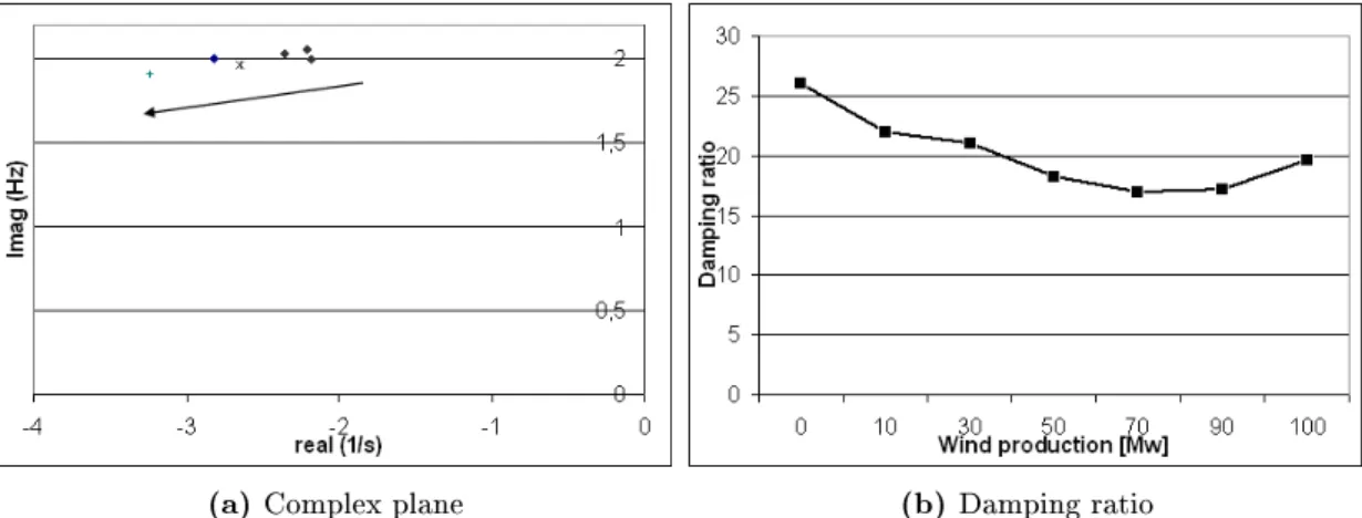
(a) Complex plane (b) Damping ratio

Figure 5.3: Eigenvalues in complex plane and with damping ratio

Figure 5.3 shows an example of how eigenvalues can be presented. Both pictures are taken from the same simulation where a wind turbine's productions is increased from 0 MW up to 100 MW. This leads to a change in the oscillatory modes of the power system. The left gure illustrates this by plotting the eigenvalues in the complex plane and the right picture plots the same eigenvalues by using the damping ratio.

5.2.6 Eigenvectors

Eigenvectors are a special set of vectors associated with a linear system of equations. Determining the eigenvectors is important in physics and engineering in order to analyze small oscillations in vibrating systems or stability analysis. Each eigenvector is paired with its corresponding eigenvalue and there are two types of eigenvectors, right eigen-vector and left eigeneigen-vector [26]. The right eigeneigen-vector dene the relative distribution of the mode throughout the system's dynamic states. It measures the activity of the state variables to an eigenvalue. The left eigenvector weights the contribution of the activity of the state variable to an eigenvalue. It gives the distribution of the states within a mode. It is for most problems sucient to only consider the right eigenvector. The term "eigenvector" used without qualication in such applications can therefore be understood to refer to the right eigenvector [24].

(45)

5.2. MODAL ANALYSIS 25 XR=      XR1 XR2 ... XRn      (5.15)

The left eigenvectorXL has the form:

XL= XL1 XL2 . . . XLn

(5.16) The eigenvectors can be normalized so that the product of the them are:

XRXL= 1 (5.17)

While the product of eigenvectors belonging to dierent eigenvalues will always be 0.

XRiXLi = 0 (5.18)

5.2.7 Participation Factors

Using right and left eigenvectors to identify the relationship between a state and a mode can be a problem since the elements of the eigenvectors are dependent on units and scaling associated with the state variables. To solve this problem a matrix called the participation matrix which combines the right and the left eigenvectors, can be used to measure the association between the state variables and the nodes [24]. The participation matrix indicates better than the eigenvectors the eect of a physical component in a system to a mode. Participation factors can by looking at generators speed participations, indicate which generators in the power system that is most suitable for power system stabilizer placement. Pi =      P1i P2i ... Pni      =      XR1iXRi1 XR2iXRi2 ... XRniXRin      (5.19)

or written in general form:

Pki =XRkiXLik (5.20)

This formula shows how one state variable contributes to one eigenvalue. This can further be used in small signal stability analysis in order to locate the source of a poorly damped eigenvalue.

(46)

26 CHAPTER 5. MODAL ANALYSIS

5.2.8 Block Diagram Representation

By laplace transforming equation 5.7 and 5.9 the following equations are obtained in the frequency domain [24]:

s∆x(s)−∆x(0) =A∆x(s) +B∆u(s) (5.21)

s∆y(s) =C∆x(s) +D∆u(s) (5.22) It is now based on the equations in the frequency domain possible to draw a power systems linearized block diagram, this is shown in gure 5.4

Figure 5.4: Block diagram representation [10]

5.2.9 Transfer Function

Transfer function representation are in contrast to the state-space representation only concerned with the input/output behaviour of the system. It is therefore possible to randomly choose state variables when a system is only specied with a transfer function and the spate-space representation is therefore in many ways a more complete description of the system.

Eigenvalue analysis of the state matrix (matrix A) is normally the best way to perform eigenvalue analysis. But since modal analysis is often done in order to construct better control designs, it is often useful to see how the open-loop transfer function is related to the state matrix and the eigenvalues.

The transfer function has the general form:

G(s) =KN(s)

D(s) (5.23)

By applying the method used in [24] it can be shown thatG(s) may be written as.

G(s) = n X i=1 Ri s−λi (5.24) where

(47)

5.3. METHODS FOR MODAL ANALYSIS 27

Ri =cXRiXLib (5.25)

Equation 5.24 now shows that the poles ofG(s) is given by the eigenvalues of matrix A.

5.3 Methods for Modal Analysis

Since an adequate model for small signal stability must include detailed information about the power system, it is not uncommon to have power system of an order of several thousands states. The eigenvalue analysis presented in the previous section would there-fore require an enormous amount of computer power and such calculations are therethere-fore limited to small-sized power system. In order to enable modal analysis of larger systems several methods have been developed [27]. This methods are further explained in this section.

5.3.1 Analysis of Small Size Power Systems

The QR-method is a widely used method to determine the eigenvalues of a matrix. This is done by applying a set of transformations to the A matrix in order to construct another matrix, say Q. Real eigenvalues will appear as diagonal elements in Q and complex eigenvalues will appear as a block diagonal 2x2 elements. When the eigenvectors of the Q matrix are found, the eigenvectors of the original matrix can be found by reversing the transformations or by inverse iteration .

Most power system analysis program's are due to computer limitations restricted to about 800 modes when using the QR method. This means that only around 80 generators can be modelled. But using the QR-method will reveal all the systems eigenvalues and eigenvectors, and it is therefore the preferred method to use if the system falls within the limitations [19].

5.3.2 Analysis of Large Size Power Systems

When a power system is to large to be analyzed using a full modal analysis, it is necessary to use partial modal analysis. Partial modal analysis virtually removes the size limita-tions for modal analysis of power systems. The only remaining limits are the programs capabilities and the availability of data.

The rst algorithm using this technique was the AESOPS [19]. This algorithm used the quasi-Newton method iteration to nd system eigenvalues close to the dened starting value and was capable of handling up to about 2000 states. The algorithm has now been replaced by other more ecient methods such as:

• Inverse iteration and generalized Rayleigh Quotient iteration • Modied Arnoldi

(48)

28 CHAPTER 5. MODAL ANALYSIS All this methods are quite similar and they all uses repetitive multiplication of a vector by the state matrix A.

Selective modal analysis on the other hand is a complete dierent method that only focuses on the relevant eigenvalues in a specic area. The method avoids having to deal with the large system matrix and can therefore greatly reduce storage and computer requirements [27].

(49)

Chapter 6

Practical use of Modal Analysis

This chapter evaluates the modal analysis technique by linearization a small power sys-tem with a synchronous generator. A MATLAB program capable of testing the syssys-tems eigenvalues, damping factors and participation factors when the network parameters are altered is presented.

6.1 Linearization of a Synchronous Generator

A synchronous generator connected to an innite bus through a line is used to illustrate the possibilities of small-signal stability studies.

Figure 6.1: SMIB system [11]

Figure 6.1 shows the single machine innite bus system. Since the system is simple, it allows linearization of formulas to be performed in an understandable way.

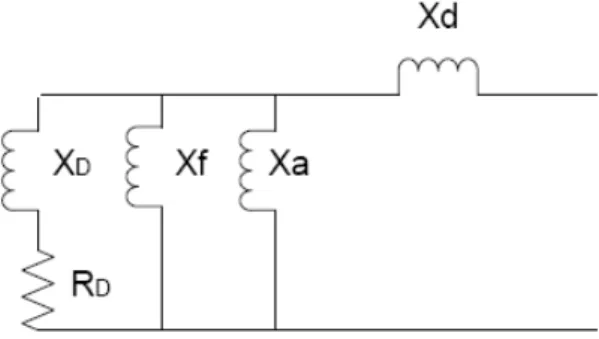
Figure 6.2: Equivalent circuit in the sub-transient state

(50)

30 CHAPTER 6. PRACTICAL USE OF MODAL ANALYSIS The equivalent circuit of gure 6.1 is shown in gure 6.2. The generator is modelled as a constant voltage source behind a reactance (Xd) and the line is modelled as a pure

reactance.

The real power produced by a generator with a salient-pole rotor (xd 6= xq) calculated

with pu units is as given by [12]:

Te=Pe= Eq Vs xd sinδ+ V 2 s 2 xd−xq xqxd sin 2δ (6.1)

When the generator uses a round rotor (xd=xq) or a classic presentation is used, formula

6.1 can be simplied to:

Te=Pe=

Eq Vs

xd

sinδ (6.2)

wherexd=Xd+Xl and xq=Xq+Xl

Most of a generators damping eect comes from the damper windings . If the rotor speed is dierent from the system frequency an emf and a current will be induced. This will produce a damping torque which will try to restore the synchronous speed of the rotor. The eect of the damper winding must therefore be included in stability analysis [12]. Figure 6.3 shows an equivalent circuit of a synchronous machine where the damping windings are given asXD

Figure 6.3: Equivalent circuit of synchronous generator [12]

The damping power can be calculated as described in [12], by using the power angle during steady state operation and the generators values for transient and sub-transient reactance and time constants. The following formula will then describe the damping power of the generator when saliency is disregarded:

KD =Vs2 X_d, −X_d,, (X+X_d,)2 X_d, X_d,, T_d,,∆ω 1 + (T_d,,∆ω)2 (6.3)

By taking saliency into account and replacing the voltage Vs in d and q by applying,

(51)

6.1. LINEARIZATION OF A SYNCHRONOUS GENERATOR 31 KD =Vs2 _X, d−X ,, d (X+X_d,)2 X_d, X_d,, T_d,,∆ω 1 + (T_d,,∆ω)2 ∗sin 2₍_δ_{) +} X , q−Xq,, (X+Xq,)2 Xq, Xq,, Tq,,∆ω 1 + (Tq,,∆ω)2 ∗cos2(δ) ∗ωs (6.4) During large speed deviations the damping power is a non-linear function of the speed deviation while it is proportional to the speed deviation when the deviation is small. A small deviation such ass= ∆ω/ωs1, would therefore allow the term (T_d,,∆ω)2 in the

denominator of formula 6.4 to be neglected. The formula can then be simplied to:

KD =Vs2 _X, d−X ,, d (X+X_d,)2 X_d, X_d,,T ,, d ∗sin 2₍_δ_{) +} X , q−Xq,, (X+Xq,)2 Xq, Xq,, T_q,,∗cos2(δ) ∗ωs (6.5)

By calculating the close loop and open loop time constants, the relationship will be:

T_d,,=T_do,, Xd, , X_d, T ,, q =Tqo,, Xq, , Xq, (6.6)

By applying this to formula 6.5 and since x,_d=X+X_d, and x,q =X+Xq,, the formula

can be simplied to:

KD =Vs2 X_d,−X_d,, (x,_d)2 T ,, do∗sin 2₍_δ_{) +}X , q−Xq,, (x,q)2 T_q,,∗cos2(δ) ∗ωs (6.7)

The dampingKD can now be calculated and used in order to nd the systems stability 6.1.1 Swing Equation

The angle between the rotor axis and the magnetic eld in a synchronous machine is known as the power angle or torque angle. When a perturbation occurs the rotor will ac-celerate or deac-celerate and a relative motion begins. The equation describing this relative motion is known as the swing equation [28].

A change from steady state due to a perturbation will result in a positive or negative torque causing acceleration or deceleration:

Ta=Tm−Te (6.8)

when including the moment of inertia ,J, and neglecting frictional damping the equation

becomes:

Jdωm

dt =Ta=Tm−Te (6.9)

This equation can be expanded to include the per unit inertia constant H, which is further explained in appendix B.2:

(52)

32 CHAPTER 6. PRACTICAL USE OF MODAL ANALYSIS

J = 2H

w₀2_mV Abase (6.10)

and the damping factorKD in pu torque/pu speed deviation, such that [24]:

2H ωo

d2δ

dt2 =Tm−Te−KD∆ωr (6.11)

Formula 6.11 is now the swing equation of a synchronous machine and it represents the swings in rotor angle (δ) during disturbances.

Since the state-space representation requires a set of rst order dierential equations , formula 6.11 must be expressed as two rst order dierential equations, which can be written in per unit as:

d∆ωr dt = 1 2H(Tm−Te−KD∆ωr) (6.12) dδ dt =ωo∆ωr (6.13) 6.1.2 Linearization

The swing equations 6.12 and 6.13 are nonlinear functions of the power angle. It is however possible to assume that they may be linearized, with little loss of accuracy, for small disturbances:

By linearizing formula 6.1 around an initial operating point where δ = δ0, the formula

can be written in linearized form as:

∆Te= ∂Te ∂δ ∆ = E0Vs xd cosδ∗∆δ+E_B2xd−xq xqxd cos(2δ) ! ∗ ∆δ=Ks∗∆δ (6.14)

and for formula 6.2:

∆Te= ∂Te ∂δ ∆ = E0Vs xd cosδ∗∆δ =Ks∗∆δ (6.15)

Ks in formula 6.14 and 6.15 is referred to as the steady state synchronising power

coef-cient and describes the generator's pull-out power. Equation 6.12 and 6.12 can now be linearized to:

f1(δ, ω) = d∆ωr dt = d2δ dt2 = 1 2H(Tm−Ks∆δ−KD∆ωr) (6.16) f2(δ, ω) = d∆δ dt =ωo∆ωr (6.17)

(53)

6.1. LINEARIZATION OF A SYNCHRONOUS GENERATOR 33 Using formula 5.8 it is ossible to nd the elements in the A and B matrix . Applying the formula to ElementA11in the A matrix yields:

∂1 ∂x1 = δ ∆ωr = = 1 2H(Tm−Ks∆δ−KD∆ωr) = 1 2H(0−0−KD) =−KD 2H (6.18)

And using the same method for the rest of the elements the complete A and B matrix will be: A= ∂f1 ∂x1 ∂f1 ∂x2 ∂f2 ∂x1 ∂f2 ∂x1 ! = −KD 2H − KS 2H ω0 0 (6.19) B = ∂f1 ∂u1 ∂f2 ∂u1 ! = ₁ 2H 0 (6.20) Which gives the following state space equation 5.7:

. ∆ω_. r ∆δ ! = −KD 2H − KS 2H ω0 0 ∆ωr ∆δ + ₁ 2H 0 ∆Tm (6.21)

The eigenvalues for the system can now according to formula 5.12 be:

det( −KD 2H − KS 2H ω0 0 −λ 1 0 0 1 ) = 0 (6.22) det −KD 2H −λ − KS 2H ω0 0−λ (6.23) −KD 2H −λ(0−λ) + ( −KS 2H ω0) = 0 (6.24) KD 2Hλ+λ 2₋−KS 2H ω0 = 0 (6.25) λ2+KD 2Hλ− −KS 2H ω0 = 0 (6.26)

(54)

34 CHAPTER 6. PRACTICAL USE OF MODAL ANALYSIS λ1,2 = −KD 2H ± q (KD 2H)2−4∗1 KS 2Hω0 2∗1 = =−KD 4H ± r (KD 4H) 2₋ KS 2Hω0 (6.27)

The general form of an eigenvalue is:

λ=σ±jω (6.28)

The real component of the eigenvalue also known as the dampingσ, and the oscillation

of the eigenvalueω will be:

σ=−KD 4H ω= r (KD 4H) 2₋KS 2Hω0 (6.29)

And the damping ratio will according to formula 5.14 be:

ζ = p −σ

(σ)2_{+ (}_ω₎2 (6.30)

The right eigenvectors are given by:

(A−λI)XR= 0 (6.31) −KD 2H − KS 2H ω0 0 −λ 1 0 0 1 XR1i XR2i = 0 (6.32)

The left eigenvectors are given by:

XR=X_L−1 =

adj(XL)

|XL| (6.33)

The participation matrix can now be found by multiplying the right and left eigenvector for each eigenvalue:

P = P1i P2i = XL11XR11 XL12XR21 XL21XR11 XL22XR22 = P11 P12 P21 P22 (6.34) The rst column of the participation matrix shows how mode 1 involves each state variable. The second column shows how mode 2 involves each state variable [11]

(55)

6.2. SMALL SYSTEM WITH SYNCHRONOUS GENERATOR 35     λ1 λ2 ∆ωr... P11 P12 ∆δ... P21 P22     (6.35)

For each mode λ1 and λ2, the participation matrix shows how each state variables, in

this caseωr and δ, is involved

6.2 Small System With Synchronous Generator

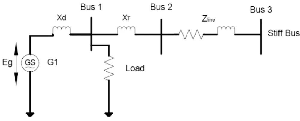
Network 1 in section 7.3 is simplied by removing Bus 2 and Bus 4. The line from Bus 5 to Bus 6 is removed and the generator is modelled as a constant voltage behind the transient reactance. The derived formulas in the previous section are used to construct a MATLAB le able to calculate all relevant values for small-signal analysis. The MATLAB code can be found in appendix A.2 and the values for the system including the generator can be found in appendix A.1.

Figure 6.4: Three bus example

6.2.1 Calculations with Initial Values

The values given for the network and the generator are used to calculate the properties of the network. By using the derived formulas all relevant values for small-signal analysis can now be calculated.

The rst thing required to nd is the Voltage at Bus 1.

The voltage at Bus 1 can be found by adding the voltage at Bus 3 and the line losses:

V1 =V3+ ∆Vline

=V3+I∗(XT +Zline)

(6.36) and the line can current be nd with:

Il=

(P1+J Q1)∗

(56)

36 CHAPTER 6. PRACTICAL USE OF MODAL ANALYSIS Combining formula 6.36 and 6.37 and ignoring the line resistance (X = XT +Xline)

yields: V1=V3+ (P1+J Q1)∗ V1 ∗X =V₁2−V3∗V1−(P1+J Q1)∗∗X = V3± p V₃2−(4∗1∗ −(P1−J Q1)∗X 2 (6.38)

And by using the predened values found in appendix A.1:

V1 = 1.0±p1.02_{+ (4}_∗₁_∗₍₀_.₅₋_J₀_.₁₎_∗_J₀_.₃₅ 2 = 1.0565 +J0.157 = 1.0686 ₈_.₄₆ (6.39)

The current trough the line can now be found using formula 6.37:

Il= (P1+J Q1)∗ V1 = (0.5 +j0.1) ∗ 1.0565 +J0.157 = 0.45−J0.161 = 0.4776 ₋₁₉_.₇₆ (6.40)

and for the local load

Il =

P1

V1

= 0.5

1.068 = 0.467 (6.41) The total current from the generator will then be

Itot =Iload+Iline

= 0.467 + 0.45−J0.161

= 0.918−J0.161 = 0.9336 ₋₉_.₉₄₇

(6.42)

The transient voltage behind the transient reactance:

E_g, =V1+J Xd, ∗Itot

= 1.0565 +J0.157 +J0.3∗(0.918−J0.161) = 1.1050 + 0.4324i= 1.1876 ₂₁_.₃₆

(6.43)

Since the generator is using a salient rotor (xd6=xq) formula 6.14 must be used to nd