Robust Detection of Multiple Sclerosis Lesions from
Intensity-Normalized Multi-Channel MRI
Yogesh Karpate, Olivier Commowick, Christian Barillot
To cite this version:
Yogesh Karpate, Olivier Commowick, Christian Barillot. Robust Detection of Multiple
Sclero-sis Lesions from Intensity-Normalized Multi-Channel MRI. SPIE Medical Imaging, Feb 2015,
Orlando, United States.
<
inserm-01127692
>
HAL Id: inserm-01127692
http://www.hal.inserm.fr/inserm-01127692
Submitted on 7 Mar 2015
HAL
is a multi-disciplinary open access
archive for the deposit and dissemination of
sci-entific research documents, whether they are
pub-lished or not.
The documents may come from
teaching and research institutions in France or
abroad, or from public or private research centers.
L’archive ouverte pluridisciplinaire
HAL
, est
destin´
ee au d´
epˆ
ot et `
a la diffusion de documents
scientifiques de niveau recherche, publi´
es ou non,
´
emanant des ´
etablissements d’enseignement et de
recherche fran¸
cais ou ´
etrangers, des laboratoires
publics ou priv´
es.
Robust Detection of Multiple Sclerosis Lesions from
Intensity-Normalized Multi-Channel MRI
Yogesh Karpate, Olivier Commowick and Christian Barillot
VISAGES: INSERM U746-CNRS UMR6074 INRIA University of Rennes I, France
ABSTRACT
Multiple sclerosis (MS) is a disease with heterogeneous evolution among the patients. Quantitative analysis of longitudinal Magnetic Resonance Images (MRI) provides a spatial analysis of the brain tissues which may lead to the discovery of biomarkers of disease evolution. Better understanding of the disease will lead to a better discovery of pathogenic mechanisms, allowing for patient-adapted therapeutic strategies. To characterize MS lesions, we propose a novel paradigm to detect white matter lesions based on a statistical framework. It aims at studying the benefits of using multi-channel MRI to detect statistically significant differences between each individual MS patient and a database of control subjects. This framework consists in two components. First, intensity standardization is conducted to minimize the inter-subject intensity difference arising from variability of the acquisition process and different scanners. The intensity normalization maps parameters obtained using a robust Gaussian Mixture Model (GMM) estimation not affected by the presence of MS lesions. The second part studies the comparison of multi-channel MRI of MS patients with respect to an atlas built from the control subjects, thereby allowing us to look for differences in normal appearing white matter, in and around the lesions of each patient. Experimental results demonstrate that our technique accurately detects significant differences in lesions consequently improving the results of MS lesion detection.
Keywords: Multiple Sclerosis, Intensity Normalization, Statistsics, MRI
1. DESCRIPTION OF PURPOSE
Multiple sclerosis (MS) is a chronic inflammatory demyelinating disease affecting the central nervous system (CNS). The disease usually affects young adults, who suffer from a variety of neurological symptoms, with periods of relapse and remission (relapsing-remitting MS), or progressively leading to irreversible disabilities (primary or secondary progressive MS). The pathophysiology of the disease is complex, and not perfectly understood at this time. Quantitative analysis of Magnetic Resonance Images (MRI) of different patients provides a spatial analysis of the brain tissues, which may lead to the discovery of putative biomarkers of disease evolution. The origin and evolution of this disease are still not well understood, and numerous studies have been conducted to evaluate its evolution and its influence on neighboring brain structures.
Although manual lesion detection by experts is the Gold Standard, the objective evaluation of lesion becomes difficult for the radiologist when the number of MR sequences grows dramatically. Consequently, several studies investigated the automatic/semi-automatic segmentation of MS lesions using MRI.1 One breed of MS lesion segmentation includes Gaussian Mixture Modeling (GMM) on multi-spectral MR images, where each multivariate Gaussian probability density function represents a tissue: e.g. cerebrospinal fluid (CSF), gray matter (GM) and white matter (WM). The GMM enables characterization of the image intensities with a reduced number of parameters which are estimated by a maximum likelihood estimator (MLE) with the Expectation-Maximization (EM) algorithm and its variants.2 The other approach contain detection based the group based comparison
between controls and MS patients. In their pioneering work of usage of Diffusion Tensor Imaging (DTI) in MS, Filipi et al.3 evaluated the differences in fractional anisotropy (FA) between MS patients and controls on
normal appearing white matter regions. Commowick et al.4 proposed the use of the whole diffusion tensor
information (DTI) to detect statistically significant differences between MS patients and controls. We propose a framework that relies on the multi-channel MRI information to detect statistically significant differences between MS patients and controls. The proposed technique is built on ideas similar to Commowick et al.4 but taking into
Further author information: (Send correspondence to Yogesh Karpate) E-mail: [email protected],[email protected]
account conventional multi-channel MRI. Such an approach provides consistent and reliable lesion detections. The proposed framework consists of two major parts. First, we describe a new intensity standardization technique for minimizing the inter subject intensity differences which may occur due to protocol variations across the scanners. Since in MS, White Matter (WM) lesions are also present in addition to healthy brain tissues, the intensities from multichannel MRI are modeled with a parametric transform using a robust GMM estimation based onγdivergence. Such a formulation allows for keeping the lesions unaffected. It provides a technique that (1) uses tissue-specific intensity information by modeling them using a robust GMM; (2) provides a consistent intensity normalization between inter subject images. The second part concerns the computation and use of an unbiased atlas of multi-channel MRI from a database of controls. Based on this atlas, we show how to compute statistical differences between a patient and the atlas using a Mahalanobis distance derived from the multi-channel MRI. Subsequently, we demonstrate its crucial role for further lesion analysis.
2. METHODOLOGY
2.1 Intensity Standardization
Given two MR images of a single MS patient at time instantt1 andt2, we seek to estimate a correction factor
such that corresponding anatomical tissues adopt the same intensity profile. We model the image intensities of a healthy brain with a 3-class GMM, where each Gaussian represents one of the brain tissues White Matter (WM), Gray Matter(GM) and Cerebrospinal fluid (CSF). We consider themMR sequences as a multidimensional image withn voxels. Each voxeli is represented as xi = [xi1...xim]. The probability of intensity xi is calculated as
follows: f(xi|θ) = 3 X k=1 πkN(µk,Σk) (1)
where the mean µk and covariance Σk define the parameters of each Gaussian of the model N(µk,Σk) along
with their mixing proportionsπk merged into parameterθ. If the proportions were known,θcould be estimated
through the Maximum Likelihood Estimator (MLE):
b θ= argmax θ L(θ) = argmax θ n Y i=1 f(xi|θ) (2)
Wherexi are considered as i.i.d. samples. However, as πk are unknown, an Expectation Maximization (EM)
algorithm5is used to estimate the parameters.
2.1.1 γ-loss Function for the Normal Distribution
The parameter estimation with classic MLE for GMM can deviate from its true estimation in presence of outliers. In MS patients, such outliers may be of crucial importance as they may denote appearing or disappearing lesions. Recently, to address these shortcomings, a modification of the MLE was proposed in order to make it more robust to outliers. The basic idea is to maximize Equation 2 in the form ofγ divergence. Notsu et al.6 proposed the
γ-loss function for the Normal distribution with mean vectorµand covariance matrix Σ.
Lγ(µ,Σ) = Σ − γ 2(1+γ) n X i=1 exp −γ 2(xi−µ) TΣ−1(x i−µ) (3)
Where|.|indicates the determinant. The bounded influence function of an estimator is an indicator of robustness to outliers. The influence function for GMM withγ loss function is bounded whereas the one for regular GMM is unbounded. As γ grows larger, bounds become tighter. For a sufficiently large γ, (γ ≥0.1), the estimating equation has little impact from outliers contaminated in the data set. Equation 3 can be casted to yield an EM style algorithm as follows.
Expectation Step. In the case of a GMM, the latent variables are the point-to-cluster assignments ki, i =
1, ..., n, one for each ofndata points. The auxiliary distribution q(ki|xi) =qik is a matrix withn×K entries.
Each row ofqi can be thought of as a vector of soft assignments of the data pointsxi to each of the Gaussian
modes. qik= πkexp −γ2(xi−µk)TΣ−k1(xi−µk) K P l=1 πlexp −γ2(xi−µl)TΣ−l1(xi−µl) (4)
Maximization Step. The maximization step estimates the parameters of the Gaussian mixture components and the mixing proportionsπk, given the auxiliary distribution on the point-to-cluster assignments computed in
the expectation step. The meanµk of a Gaussian mode is obtained as the mean of the data points assigned to
it (accounting for the strength of the soft assignments). The other quantities are obtained in a similar manner, yielding to: µk = Pn i=1qikxi Pn i=1qik (5) Σk = (1 +γ) Pn i=1qik(xi−µk)(xi−µk) T Pn i=1qik (6) πk = Pn i=1qik Pn i=1 PK l=1qil (7) 2.1.2 Selection of Parameter γ
The estimation of power indexγ plays a critical role in our approach, sinceγ affects the estimated parameters in presence of outliers. The selection ofγwas studied as a model selection problem based on Akaike information criterion (AIC).6LetKbe the number of clusters,pbe the total numbers of parameters of a model and (µ
k,Σk),
k= 1, .., K be the means and the covariance matrices of the clusters respectively. From Equation 2, the AIC is defined as follows: AICγ =−2 n X i=1 logfγ(xi|θ) + 2 Kp(p+ 3) 2 +K−1 (8)
The value of γwhich minimizes AIC is used as the optimalγ. For various values ofγ, Equation 8 is evaluated in cross validation manner and the γwhich results in minimum value is chosen for the experiment.
2.1.3 Intensity Correction
We obtain the means and covariances of tissues for the source and target images using the procedure mentioned above. We chose a linear correction function such that g(x) = Σiβixi. The coefficients βi are estimated to
minimize the following cost function: Σll==1n(g(µsource,k)−µtarget,k)2. l denotes the number of voxels in classk.
This function can be solved by linear regression. Using the results of the linear regression, the intensity profiles of the two images are normalized by mapping the intensity of the source image to the target image. The resulting correction function is smooth and interpolates the intensity correction.
2.2 Multiple Sclerosis Lesions (MSL) Detection
The second part of our framework relies on the voxel-wise comparison of multi-channel MRI of MS patient against a set of controls. Here, we assume that all images (patients and controls) are aligned into a common space where each voxel of each image describes the exact same spatial position. Commowick et al.4 introduced
We aim at comparing, for each voxel, the patient vector of intensities xq and intensity vectors from control
subjectsxq, q= 1, ..., M. The control populationX=xq, q= 1, ..., M is assumed to follow a multivariate Normal
distribution N( ¯X,ΣX), where ¯X,ΣX denote respectively the average and covariance matrix of population X.
Following this assumption, we compute the difference statistic between xq and N( ¯X,ΣX) as a Mahalanobis
distance as
d2(xq) = (xq−X¯)TΣ−X1(xq−X¯) (9)
whered2will vary between 0 and +∞, getting smaller as the patient vector gets likely to belong the multivariate
Normal distribution of the controls. A p-value can then be computed from this distance as the statistic T =
M(M−h)
h(M2−1)d
2 follows a Fisher distribution with parametershand M −h: T ∼F(h, M−h)wherehis the vector
dimension (1 for scalar images). The difference test p-value is therefore written as:
p(xq) = 1−Fh,M−h M(M−h) h(M2−1)d 2(x q) ! (10)
where Fh,M−h is the cumulative distribution function of a Fisher distribution with parameters h and M −h.
Finally, as we are computing voxel-wise comparisons, a final step is to correct for multiple comparisons utilizing FDR correction as introduced by Benjamini et al.7
3. EXPERIMENTS & RESULTS
Whole-brain MR images were acquired on 16 MS patients and 20 controls. T1-w MPRAGE, T2-w and FLAIR modalities were chosen for the experiment. Expert annotations of lesions were carried out by an expert radi-ologist on all MS patients. The volume size for T1-w MPRAGE and FLAIR is 256×256×160 and voxel size is 1×1×1mm3. For T2-w, the volume size is 256×256×44 and voxel size is 1×1×3mm3. All imaging experiments
for this study were performed on a 3T Siemens Verio (VB17) scanner with a 32-channel head coil. MR images from each patient are de-noised,8 bias field corrected9and registered with respect to T1-MPRAGE volume.10, 11
All the images are processed to extract intra-cranial region.12 We built a geometrically unbiased atlas for each
sequence from dataset of controls.13 For each MS patient, nonlinear registration of the T1-w MPRAGE image onto the atlas was done.14 Patient to atlas registration consists in two steps. First, a global affine transformation was computed between the T1 images. Then, nonlinear registration was performed to locally align the anatomies of the atlas and the patient. The final transformations were then applied to T2-w and FLAIR images.
3.1 Lesion Detection Evaluation
We built a composite vector image for each patient and control from T1-w MPRAGE, T2-w and FLAIR. The atlas is considered as the reference image to which all controls and patients images are aligned using intensity normalization as described in Section 2.1.3. Finally, we applied our framework (Section 2.2) to compare the differences in images and report the results in the next section.
We performed experiments of lesion detection, to enhance the interest of our approach with respect to (1) intensity normalization and (2) to combine several modalities for lesion detection. To this end, we compared detections using each individual sequence i.e. T1-w MPRAGE, T2-w or FLAIR individually with and without intensity normalization; and then on composite vector images formed from all sequences with and without intensity normalization. The detections obtained are compared with the ground truth using Dice scores.
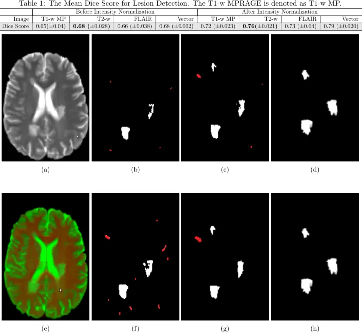
3.1.1 Quantitative Results
We report in Table 1, the Dice score average across 16 patients for each test variant. The lesion detection on different sequences are compared against each other. We report the best mean Dice score which is of T2-w as 0.76(±0.021). From Table 1, it is clear that intensity normalization plays crucial role in our framework. The lesion detection of T2-w achieves good performance because some lesions may not be found on T1-w MPRAGE and FLAIR. In Table 1, we report the mean Dice score of 0.79(±0.020) on vector images with intensity normal-ization and 0.68(±0.024) without intensity normalization, which shows a clear improvement on the best detection score from individual modalities.
Table 1: The Mean Dice Score for Lesion Detection. The T1-w MPRAGE is denoted as T1-w MP. Before Intensity Normalization After Intensity Normalization
Image T1-w MP T2-w FLAIR Vector T1-w MP T2-w FLAIR Vector Dice Score 0.65(±0.04) 0.68 (±0.028) 0.66 (±0.038) 0.68 (±0.002) 0.72 (±0.023) 0.76(±0.021) 0.73 (±0.04) 0.79 (±0.020)
(a) (b) (c) (d)
(e) (f) (g) (h)
Figure 1: Top row : A slice of MRI from T2-w Sequence (a), MSL detection obtained by without intensity normalization (b), MSL detection with intensity normalization (c) and corresponding ground truth (d). Bottom row : A slice of MRI from composite vector image (e), MSL detection obtained without intensity normalization (f), MSL detection with intensity normalization (g) and corresponding ground truth (h). White label shows the true positives where as red label indicates the false positives.
3.1.2 Qualitative Results
Figure 1 shows the lesion detection results for T2-w and composite vector image. Each row represents the image and each column depicts the anatomical slice of patient MRI, corresponding ground truth, lesion detection results without and with intensity normalization respectively. The white labels show the true lesions detected while red ones indicate the brain tissues which are detected as lesion but actually are not part of the lesions. This figure demonstrates visually the ability of our approach to detect lesions. As seen from the last two columns, there is considerable improvement of lesion detection, thanks to intensity normalization.
4. NEW OR BREAKTHROUGH WORK TO BE PRESENTED
A novel paradigm for detection of MS lesions has been proposed. We devised a two layers strategy, first intensity standardization of images with respect to an atlas; and then computation of difference scores of a specific patient to a population of controls. Such comparisons allowed the accurate detection of lesions or other diffuse pathology-related changes.
5. CONCLUSION
We proposed a new framework for MS lesion detection based on differences between multi-channel MRI of patients and controls. This framework fused with intensity standardization was applied to the study of MS and highlighted the great interest of quantitative MRI measurements made on MRI for a better understanding and characterization of the disease. The efficacy of our method was evaluated though detection with and without intensity correction. Compared to un-normalized images, detection with intensity correction is a better choice for MS lesion analysis thanks to its ability to preserve the intensity variations caused by pathological changes while normalizing healthy tissue intensities. The resulting system is both efficient and accurate. This performance suggests that it can provide valuable assistance in detecting MS lesions in clinical routine with high reliability. Our models are already capable of detecting highly variable lesion patterns, but we would like to move towards richer models. The framework described here allows for exploration of additional MR sequences with or without contrast agents. For example, one can consider infusing T1-w Gadolinium.
ACKNOWLEDGMENTS
This work was supported by the Region Council of Brittany of France and France Life Imaging (FLI) through the ANR-11-INBS-00006 grant.
REFERENCES
[1] Llad´o, X., Oliver, A., Cabezas, M., Freixenet, J., Vilanova, J. C., Quiles, A., Valls, L., Rami´o-Torrent´ı, L., and Rovira, ı., “Segmentation of multiple sclerosis lesions in brain mri: A review of automated approaches,”
Inf. Sci.186, 164–185 (Mar. 2012).
[2] Garca-Lorenzo, D., Prima, S., Arnold, D. L., Collins, D. L., and Barillot, C., “Trimmed-likelihood estimation for focal lesions and tissue segmentation in multisequence mri for multiple sclerosis.,” IEEE Transactions on Medical Imaging 30(8), 1455–1467 (2011).
[3] Filippi, M., “Diffusion tensor magnetic resonance imaging in multiple sclerosis.,”Neurology56(3), 304–3011 (2001).
[4] Commowick, O., Fillard, P., Clatz, O., and Warfield, S. K., “Detection of DTI white matter abnormali-ties in multiple sclerosis patients,” in [Proceedings of the 11th International Conference on Medical Image Computing and Computer Assisted Intervention (MICCAI’08), Part I],LNCS5241, 975–982 (Sept. 2008). [5] Dempster, A., Laird, N., and Rubin, D., “Maximum likelihood from incomplete data via the EM algorithm,”
J. of the Royal Statistical Society. Series B39(1), 1–38 (1977).
[6] Notsu, A., Komori, O., and Eguchi, S., “Spontaneous clustering via minimum gamma-divergence,” Neural Computation 26(2), 421–448 (2014).
[7] Benjamini, Y. and Hochberg, Y., “Controlling the false discovery rate: A practical and powerful approach to multiple testing,”Journal of the Royal Statistical Society Series B (Methodological)57(1), 289–300 (1995). [8] Coup´e, P., Yger, P., Prima, S., Hellier, P., Kervrann, C., and Barillot, C., “An optimized blockwise nonlocal means denoising filter for 3-D magnetic resonance images,”IEEE Transactions on Medical Imaging 27(4), 425–441 (2008).
[9] Tustison, N., Avants, B., Cook, P., Zheng, Y., Egan, A., Yushkevich, P., and Gee, J., “N4ITK: improved N3 bias correction,”IEEE Transactions on Medical Imaging29(6), 1310–1320 (2010).
[10] Ourselin, S., Roche, A., Prima, S., and Ayache, N., “Block matching: A general framework to improve robustness of rigid registration of medical images,” in [MICCAI], LNCS1935, 557–566 (2000).
[11] Commowick, O., Wiest-Daessl´e, N., and Prima, S., “Block-matching strategies for rigid registration of multimodal medical images,” in [ISBI], 700–703 (2012).
[12] Smith, S. M., “Fast robust automated brain extraction,”Human Brain Mapping17, 143–155 (nov 2002). [13] Guimond, A., Meunier, J., and Thirion, J.-P., “Average brain models: A convergence study,” Computer
Vision and Image Understanding 77(2), 192–210 (2000).
[14] Commowick, O., Wiest-Daessl, N., and Prima, S., “Automated diffeomorphic registration of anatomical structures with rigid parts: Application to dynamic cervical MRI,” in [Medical Image Computing and Computer-Assisted Intervention (MICCAI’12)], (Oct. 2012).