Local Search and Constraint Programming for the Post
Enrolment-based Course Timetabling Problem
?Hadrien Cambazard, Emmanuel Hebrard, Barry O’Sullivan and Alexandre Papadopoulos
Cork Constraint Computation Centre
Department of Computer Science, University College Cork, Ireland
{h.cambazard|e.hebrard|b.osullivan|a.papadopoulos}@4c.ucc.ie
Abstract. We present a study of the university post-enrolment timetabling prob-lem, proposed as Track 2 of the 2007 International Timetabling Competition. We approach the problem using several techniques, particularly local search, con-straint programming techniques and hybrids of these in the form of a large neigh-bourhood search scheme. Our local search approach won the competition. Our best constraint programming approach uses an original problem decomposition. Incorporating this into a large neighbourhood search scheme seems promising.
1
Introduction
Timetabling problems have a wide range of applications in education, sport, manpower planning, and logistics. A diverse variety of university timetabling problems exist, but three main categories have been identified [5, 9, 26]: school, examination and course timetabling. The Post Enrolment University Course Timetabling Problem [17] occurs in an educational context whereby a set of events (lectures) have to be scheduled in timeslots and located in appropriate rooms. The problem tackled in this paper was pro-posed as part of the 2007 International Timetabling Competition organised by PATAT (Track 2)1. The problem was also used in the 2003 competition without two specific
hard constraints introduced in 2007, which are discussed in Section 2. These new con-straints were introduced in the 2007 competition in order to make the search for fea-sible timetables difficult. In 2003 finding feafea-sible timetables was relatively easy and all algorithms, therefore, focused on optimising the soft constraints. According to the organisers [17], the two constraints have been added to move the competition closer to real-world timetabling where finding feasible timetables can be a very challenging task. This context seemed a good opportunity to investigate Constraint Programming (CP) techniques, and compare them with the strong local search baseline developed dur-ing the 2003 challenge. Ourmain contributionin this paper is a comprehensive study of the problem using a wide range of techniques highlighting both pitfalls and positive results. Our main technical novelty lies in the analysis of complete approaches with
?
This work was supported by Science Foundation Ireland (Grant Number 05/IN/I886). 1http://www.cs.qub.ac.uk/itc2007/
original CP models and lower bounds for the costs associated to the soft constraints, including algorithms to maintain them. We also present an original local search ap-proach that can deal with the hardness of feasibility; this was ranked first out of thirteen teams in Track 2 of the 2007 International Timetabling Competition. Finally, a promis-ing large neighbourhood search (LNS) scheme [27] is proposed, which contrasts with all previous published local search work on this problem [1, 6, 10, 15, 24].
2
Problem Description
The post enrolment-based course timetabling problem consists of a set ofnevents,E, to be scheduled in 45 timeslots{1, . . . ,45} (5 days of 9 hours each) using a set of mrooms,R. Each room is characterised by its seating capacity, which we will refer to as its size, and a set of features defining the set of services available in each room. Each event needs a room whose size is larger than the number of students attending the event, and it must be placed in a room with the required features. Additionally, a set of precedence requirements state that some events must occur before others. We are also given a setS of students and the set of events each must attend. Each event must be assigned to a room in a timeslot while obeying a set of constraints. The constraints of the problem are partitioned into two sets: thehardconstraints define the requirements of a feasible timetable, while thesoftconstraints define an optimal timetable. The hard constraints are the following:
1. No student can attend more than one event at the same time.
2. In each case the room has to be big enough for all the attending students and satisfy all of the features required by the event.
3. Only one event is put into each room in each timeslot.
4. An event can only be assigned to its pre-defined “available” timeslots. 5. When specified, events have to occur in the correct order in the week.
Because feasibility can be very difficult to achieve, the organisers of the competition have introduced the notion of “distance to feasibility” to be able to discriminate entries that do not find any feasible solution. We will ignore this point in our study and consider all infeasible solutions as mere failures2. The quality of a feasible timetable is evaluated
in terms of the soft constraints. A feasible solution is penalised equally if a student: 1. attends an event in the last timeslot of the day ({9,18,27,36,45});
2. attends more than two events in a row on a given day; one penalty is counted for each event attended consecutively after the first two;
3. attends exactly one event during a day.
The problem defined by the hard constraints only can be seen as a constrained list-colouring in a graph where a node is an event and an edge is added between two events that must go to different timeslots. This graph is primarily made of many large over-lapping cliques, referred to asstudent cliques, defined by the set of events chosen by each student. It can also be worthwhile to notice that two events that share a unique
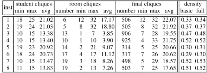
Table 1.Some statistics about the colouring graph structure in the first eight instances. inst student cliques room cliques final cliques density
min max avg number min max avg number min max avg basic full 1 18 25 21.02 6 12 32 17.17 506 12 32 22.07 0.33 0.34 2 19 24 21.03 5 8 32 18.80 505 8 32 21.92 0.37 0.37 3 10 15 13.38 13 1 7 3.85 906 7 28 19.55 0.47 0.48 4 10 15 13.40 10 1 10 3.90 925 4 33 21.75 0.52 0.52 5 19 23 20.92 14 2 21 9.07 314 5 25 20.66 0.30 0.31 6 18 24 20.73 17 4 17 11.12 317 7 26 20.62 0.29 0.30 7 10 15 13.47 19 3 18 8.26 498 5 29 18.57 0.52 0.53 8 11 15 13.83 19 2 13 7.26 503 7 25 17.65 0.51 0.52
possible room, due to their size and features, have to be assigned to different timeslots. The cliques relying on those edges are referred to asroom cliques. At last, precedences also imply differences and can be added in the graph. Table 1 gives some details about the size and number of cliques found in the colouring graph because both our LS and CP approaches will try to take advantage of them. It also shows the density of thebasic graph, i.e. the original graph of student choices including the precedence edges, and the fullgraph, i.e. the same graph augmented with rooms.
Thefinal cliquesof Table 1 are obtained by the following process: the neighbour-hood of a cliquec,i.e.the set of nodes connected to all the nodes ofc(but not necessarily with each other) can intersect another clique, and the corresponding intersection can, therefore, be used to extendc. The final cliques are obtained by applying such a pro-cess iteratively from the student/room cliques until a fixed point is reached. The density of the full graph is not much bigger than for the basic graph, but the added edges can significantly improve the maximum and average size of the cliques.
3
A Local Search Approach
Our local search baseline is strongly based on the work achieved during the 2003 com-petition and the improved results published later in [6, 15, 24]. There are, however, some differences to consider due to the increased difficulty of finding feasible timetables in the 2007 competition instances. Similar to most approaches of 2003, our local search is performed in two steps: we first try to identify a feasible solution, and then try to reduce the cost of violating the soft constraints. The originality of our local search lies mainly in finding feasible timetables. We describe both steps in more detail below.
3.1 Finding Feasible Solutions
The search for feasible solutions is performed by considering a unit cost per hard con-straint violation: an infeasible timeslot or room for an event, two events sharing a stu-dent in the same timeslot, two events violating a precedence between them.
Representation of the solution. Thepositionof an event is defined by a given timeslot and room. The solution is represented by the position of each event as opposed to the solution representation described in [24], which ignores the rooms and maintains the room violations by solving a matching problem per timeslot. Knowing if a set of events can fit in a given timeslot with respect to room availability and capacity is a
bipartite matching problem (events to rooms). For efficiency reasons, the lists of events per timeslot as well as the list of all free positions in the timetable (positions where no event is currently assigned) are added to the representation.
Neighbourhood. The neighbourhood can be seen as a composite neighbourhood struc-ture [1, 10] defined in terms of the following moves:
1. T rE: translates an event to a free position of the timetable.
2. SwE: swaps two events by interchanging their position in the timetable.
3. SwT: swaps two timeslotstiandtj,i.e.translates all events currently placed inti
totjand all events intjtoti.
4. M a(Matching): reassigns the events within a given timeslot to minimise the num-ber of room conflicts; to allow violations, a maximum matching is solved.
5. T rE+M a: translates an event to a timeslot and evaluates if this does not violate the room constraints by checking the corresponding matching problem; if the matching is infeasible, the move is rejected.
6. Hu(Hungarian): picks a set of events{e1, . . . , ek}assigned in different timeslots
(k≤45) that do not have precedences defined between them, and reassigns them optimally by solving an assignment problem with the Hungarian algorithm [16]. The violation of the hard constraints for placing each event in each timeslot is known as it does not depend on the other removed events, since they do not share precedences and only a single event is removed per timeslot. We solve45×k max-imum matching problems to evaluate the cost due to the room capacities of placing each event in each timeslot. As the number of such moves is exponential, the size of the neighbourhood is restricted toKsets (K = 20in practice), including con-flicting events (involved in hard constraints violations) and completed randomly. T rEandSwTare always considered in the neighbourhood. The remaining moves are ranked in terms of their time complexities and included in the neighbourhood at a given iteration depending on a probability related to their complexity. More specifically, the probabilities are set top(Hu) =p(SwT) = 1054,p(M a) =
1
103,p(T rE+M a) =
1
102. Thus, time consuming moves are performed less frequently than faster ones. The
set of moves considered at each iteration, therefore, varies and the order of explo-ration amongst them is chosen randomly. However, for each move the exploexplo-ration is performed deterministically from the last point where it was left (similar to [15]). Search. Improving and sideways moves, which keep the current violation cost constant, are always accepted and no emphasis is put on conflicting events, except by moveHu. We believe that movesT rE andSwE are very important in our approach. They can be performed very quickly and, therefore, provide a diversification mechanism as the search is not guided by conflicting events. This also explains why we choose a solution representation that includes the room information explicitly, since this is mandatory for T rE andSwE. A simple tabu list of sizek = 10prevents cycling by forbidding an event being considered in a timeslot it was assigned in the lastkiterations; this is similar to [6] and classic in graph colouring [11]. Finally, a pure random configuration is used to start as we found no significant benefits to starting from a greedy solution.
Intensification. As mentioned previously, the problem defined by the hard constraints can be seen as a constrained list-colouring problem in which the graph is made of many overlapping large cliques (see Table 1). The intensification step tries to take advan-tage of the presence of such large cliques by iteratively applying move Huon each clique containing at least one conflicting event. All events of the clique have to be in different timeslots and define an assignment problem in the current timetable. This in-tensification is applied every 50000 non-improving iterations. All cliques containing a conflicting event are considered, and simplified to ignore any precedences amongst the events inside the clique. This step is applied on all the “final cliques” of Table 1. Results. Table 2 compares a local search LS1 with a neighbourhood based only on the moves{T rE, SwE, M a, T rE+M a}with the full scheme, LS2, described previously (involving a richer and randomised neighbourhood as well as the intensification step). All instances except instances 1,2,9 and 10 seem quite easy from the point of view of feasibility, and the efficiency of our improvements can be mainly seen on instances 2,9 and 10, which are much more challenging. The diversification given by the randomised neighbourhood (by favouringT rEandSwE), and the intensification given byHuand its systematic use on the cliques, is beneficial for the hard instances. Table 2 shows the percentage of feasible solutions found over 100 runs with different seeds within the time limit3and the average time required by LS1 and LS2, which is computed only on runs
that have found a solution. Instance 10 is the only instance that remains really “open” for feasibility as all others are solved more than 94% of the time.
Table 2.Percentage of solutions found, with average time, using a simple Local search (LS1) and our improved scheme (LS2).
Instances 1 2 3 4 5 6 7 8 9 10 11 12 13 14 15 16 LS1 % solved 100 70 100 100 100 100 100 100 92 17 100 100 100 100 100 100 avg time (s) 35.9 240.7 1.1 0.9 5.1 5.4 5.3 2.6 169.5 385 0.9 1.5 10 7.7 1 0.7 LS2 % solved 100 94 100 100 100 100 100 100 95 33 100 100 100 100 100 100 avg time (s) 30.4 127.9 2 1.9 5.9 7.8 8 6.6 116.3 355 0.8 1.3 6.8 7.5 1.3 1.1
3.2 Finding Good Solutions
Once a feasible solution has been found, another local search optimises its soft cost. Representation of the Solution. We extend the previous representation by adding the student view. The timetable of each student (needed for cost 2) is kept as a three dimen-sional matrix of size|S| ×5×9where each entry is equal to the event attended by the student at the corresponding day and timeslot (if there is one, and set to -1 otherwise). Moreover, the number of events attended by each student, each day, is stored for cost 3. Neighbourhood. The only move used in this phase isT rE+M a. Moreover, the moves considered are only those preserving feasibility. We note that this is a severe disadvan-tage for the search due to the tightness of the hard constraints. The main motivation for the LNS approach of Section 6 is to compensate for this disadvantage.
3
These experiments were run on a MacBook (2 GHz Intel Core Duo, 2 GB 667 Mhz DDR2) with a time limit of 420s given by the benchmarking system of the competition.
Search. The tabu search appears inefficient for the soft cost and better results are obtained using simulated annealing (SA) [14]. This seems to match the experience of [6, 15] and the study made in [24]. Improving and sideways moves are always per-formed and degrading ones are accepted with a probability depending on their cost variation∆:Pacceptance(∆, τ) = e−
∆
τ where the parameterτ, the temperature,
con-trols the acceptance probability and is decreased over time. The temperature iscooled at each step using a standard geometric coolingτn+1= 0.95×τn. Two parameters are
needed to define the cooling: the initial temperatureτ0, and the length of a temperature
step,L,i.e.the number of iterations performed at each temperature level. As the time demand varies a lot from one instance to the other, we try to predict “the speed” of our soft solver during an initialisation phase by running the SA at a temperature of 1 for 20000 iterations and setτ0andLin the following way. Firstly,τ0is set to the average
of the cost variation observed during the initialisation; then, based on the time needed to perform the initialisation, we get an estimation of the number of iterations that will be performed in the remaining time,I. By setting a final temperature toτf = 0.2, we
also know the number of temperature step,nbSteps, needed to go fromτ0 toτf and
thereforeLis set to L = nbStepsI . A reheating is performed if the neighbourhood is scanned without accepting any moves. This can happen if the number of feasible moves is limited and the SA is more likely to reject all choices as the temperature decreases.
3.3 A Synthesis of the Local Search Approach
We conclude the presentation of the local search approach by showing the behaviour of the search at the two stages,i.e.feasibility and optimisation on the plots of Figure 1.
0 5 10 15 20 10000 20000 30000 40000 50000 60000 cost number of iterations
(a) Tabu search - feasibility stage
0 500 1000 1500 2000 2500 3000
500000 1e+06 1.5e+06 2e+06 2.5e+06 3e+06
cost
temperature
number of iterations violation cost
temperature
(b) Simulated Annealing - optimisation stage Fig. 1.Evolution of the violation cost per iteration for the two stages of the local search approach.
Both plots show the evolution of the costs at each iteration. The cooling is also indicated for the SA. The search for feasibility proceeds by moving over a large plateau of configurations of equivalent violation cost,i.e.the cost is never degraded in practice. Sideways moves appear to be very frequent for feasibility. Therefore, the search can stay for a long time on the same plateau as it does not focus on conflicting events and accept
any sideways step; this is why favouring movesT rEandSwE brings diversification over the plateau. Therefore, the role of the intensification step is important.
Sideways moves are less likely to occur at the optimisation stage and one can see the effect of the cooling by observing that the cost variation is decreasing while the best known cost is converging toward its final value. The choice of the different metaheuris-tics for feasibility and optimisation, with their resulting behaviours, is also motivated by the fact that, in the first case, we try to get a feasible solution as soon as possible whereas in the second case we aim for the best possible solution within a given time-limit.
4
Constraint Programming Models for Feasibility
This timetabling problem was tackled by a number of local search techniques [1, 6, 10, 15, 24]. We are not aware, however, of any complete approach. We considered several CP models, none of which were able to match the efficiency of local search. However, as we shall see in Section 6, the CP approach can still be valuable to provide com-plex neighbourhoods within the SA algorithm. We present here the most promising CP model as well as two less successful ones and give some insights into their inefficiency.
4.1 Basic Model
For an eventiwe introduce two variableseventT imei∈ {1, . . . ,45}andeventRoomi ∈
{1, . . . , m}, for the timeslot and room associated to eventi, respectively. LetRibe the
set of rooms that can accommodate eventi,Tibe the set of timeslots available for event
i,student(i)be the set of students attending eventiand, finally, letprecbe the set of the pairs of ordered events. We define the first model as follows:
Model 1
∀i, j≤ns.t.student(i)∩student(j)=6 ∅ eventT imei6=eventT imej (1)
∀i≤n eventRoomi∈Ri(2)
∀i, j≤n (eventT imei6=eventT imej)∨(eventRoomi6=eventRoomj)(3)
∀i≤n eventT imei∈Ti(4)
∀(i, j)∈prec eventT imei< eventT imej (5)
In this viewpoint, the constraints (1), (4) and (5) correspond to alist colouringproblem with precedences on the variables eventT ime. Constraints (2) and (3) enforce that events be allocated to suitable rooms, and that within a given timeslot, every event be put into a different room, respectively. They correspond to a set ofmatchingproblems, one for each timeslot, conditioned by the result of the above colouring problem. An important observation is that these two aspects are relatively disconnected. Indeed, as long as an event is not committed to a given timeslot, we do not know in which matching it will participate because of the disjunctions (3). If an early decision on the colouring part prevents a consistent room allocation, it will not be discovered until very late in the search, leading to atrashingbehaviour where large unsatisfiable subtrees are explored again and again. We explored two ways of resolving this issue. First, we modelled the relation between the room allocation (matching) and timeslot allocation (colouring) using a global constraint [2] to achieve stronger inference between these two aspects
and detect mistakes earlier. We describe this model in Section 4.2. The second solution was to separate the solving of the colouring and the matchings, so that we explore more diverse colourings, and hopefully avoid trashing. We describe this model in Section 4.3.
4.2 Matching Constraint
Knowing if a set of events can fit in a given timeslot with respect to room availability and capacity is a bipartite matching problem (events to rooms). The objective is to remove theeventRoomvariables from the search space. In other words, we will make sure that constraint propagation alone ensures that an assignment of all events can be extended to a matching for each timeslot. As a result, we solve a colouring problem where we only assign events to timeslots subject to timeslot availability, precedences and such that the remaining matching sub-problems are backtrack-free.
The room allocation sub-problem can be represented in a bipartite graph G = (V1, V2, E)whereV1={1, . . . , n}is the set of events, andV2={h1,1i, . . . ,h45, mi}
is the set of all pairshtimeslot, roomi. An edge(i,hj, ki)is present iff eventican be assigned to timeslotj in room k. A maximal matching ofG thus represents an as-signment of events to rooms satisfying constraints (2) and (3). We introduce n vari-ables to link this matching with the colouring. eventi ∈ {h1,1i, . . . ,h45, mi}
de-notes the timeslot and room, represented by a pair, to which event iis assigned. An
ALLDIFF({event1, . . . , eventn})[22] makes sure that the graphGadmits a matching
of cardinalityn. Notice that during search, arc-consistency is achieved for all matching problems at once, giving stronger inference than considering matchings independently. Notice that we could post other constraints directly on variablesevents. However, this can be done more easily on theeventT imevariables. They also provide a naturally good branching scheme, since rooms have been factored out of the search space. We thus define a second model, where we substitute the variableeventRoomiwitheventi
and channel it toeventT imeiusing a simple binary constraint.
Model 2
∀i, j≤n s.t student(i)∩student(j)6=∅ eventT imei6=eventT imej(1)
∀i≤n eventT imei∈Ti(4)
∀(i, j)∈prec eventT imei< eventT imej(5)
∀i≤n eventi∈ hRi×Tii(6)
∀i≤n eventT imei=eventi[0](7)
ALLDIFF({event1, . . . , eventn})(8)
Constraint (7) channels the variableseventT ime toeventby projecting on the first element of the pair. Notice that since arc consistency is achieved in polynomial time on the ALLDIFFconstraint, an assignment ofeventT imesatisfying Model 2 can always be extended toeventin a backtrack-free manner.
4.3 Alternate Colourings and Matchings
Constraint (8) of Model 2 is very costly to maintain. Therefore, we consider a decom-position similar to a logic-based Benders decomdecom-position scheme [12]. We delay the resolution of the matchings once a colouring has been found. If the matching is infeasi-ble, we seek another solution for the colouring sub-problem, and iterate in this way until
a full solution is found. Clearly, solving the colouring part alone allows for a far more optimised and sleeker model, however, reaching a fixed point might not be easy. We first describe the lighter model restricted to the colouring and precedence constraints, and where the room allocation constraints are relaxed to a simpler cardinality constraint. Then, we show how Benders cuts can be inferred when failing to solve a matching in order to tighten the colouring sub-problem.
TheeventRoomvariables are ignored as in the previous model and a single global cardinality constraint (GCC) [23] is added to ensure that every timeslot is used at most mtimes. This constraint eliminates trivially infeasible matchings where the number of events assigned to a timeslot is greater than the number of rooms.
Model 3
∀i, j≤n s.t. student(i)∩student(j)6=∅ eventT imei6=eventT imej(1)
∀i≤n eventT imei∈Ti(4)
∀(i, j)∈prec eventT imei< eventT imej(5)
∀i≤n GCC({eventT imei|i≤n},[[0..r], . . . ,[0..r]])(9)
A solution of this model is not guaranteed to be a feasible solution of the original prob-lem. Indeed, a matching problem can be inconsistent once the colouring is fixed. We, thus, iteratively solve the colouring part until we find a feasible room allocation, as de-picted in Algorithm 1. If a matching problem fails, a minimal conflict corresponds to a set of events that cannot be assigned together in any timeslot, whilst forming an in-dependent sub-graph of the colouring graph. We use an algorithm for finding minimal conflicts [8] to extract such a set of events (line 3). In order to rule out this conflicting as-signment in future resolutions of the colouring sub-problem, we post a NOTALLEQUAL
constraint to the model (line 4). The constraint NOTALLEQUAL(x1, . . . xk)ensures that
there existsi, j ∈ [1..k]such thatxi 6= xk. It acts as a Benders cut and prevents the
same assignment from being met again. Observe that since we extract minimal sets of conflicting events [4, 13], entire classes of assignments that would fail for the same rea-son are ruled out. Notice also that although this constraint is inferred from a particular timeslot, it holds for every timeslot.
Algorithm 1:Decomposition 1 repeat 2 solve Model 3; matched←true; foreach1≤j≤45do G←(V1={i|eventT imei=j}, V2=Si∈V 1 Ri, E={(i, k)|i∈V1, k∈Ri}); ifcannot find a matching ofGthen
matched←false;
3 cut←Extract-min-conflict(G);
4 add NOTALLEQUAL(eventT imek|k∈cut)to Model 3;
untilmatched;
We explored further improvements of this model based on the analysis of the colour-ing graph described in Section 2. Conflicts between events are organised into large cliques, one for each student and even larger cliques can be inferred by taking room
conflicts into account. This information can be used to obtain stronger filtering from the model. One possibility is to replace the constraints (1) by ALLDIFF constraints.
Each of the aforementioned “final cliques” implies an ALLDIFF constraint between a set ofeventT imeivariables. In this manner, all the binary differences(1)are covered
by at least one clique and can thus be removed. We can expect to achieve a stronger level of propagation as a result. On the other hand, ALLDIFFcan be expensive to maintain. We can therefore choose to keep, amongst the final cliques, only the cliques obtained from a room clique, as a trade-off between the efficiency of binary differences and the additional reasoning brought by the cliques, as they are big and they contain additional conflicts. This leads to two variations of Model 3 that we assess empirically below.
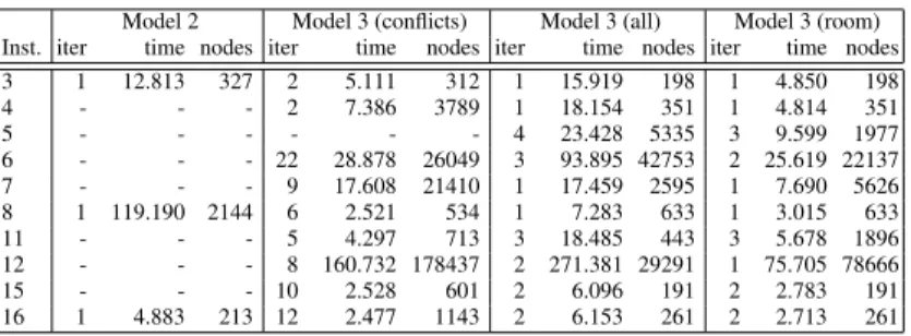
4.4 Experimental Results
We ran Model 2, Model 3, Model 3-cliques (Model 3 including all implied ALLDIFF
constraints) and Model 3-rooms (Model 3 including only the ALLDIFF constraints standing for room cliques). In Table 3, we give the number of iterations of Algorithm 1 (Decompositon), that is, the number of feasible colourings that were required to find a complete solution. This number is always 1 for Model 2. We also give the cumulative CPU time and number of nodes explored on solved instances. Notice that no model could solve instances 1, 2, 9, 10, 13 or 14 within the time cutoff of 420 seconds, corre-sponding to the 10 minutes cutoff of the competition on an Apple MacBook. Model 2 does not need to solve several colouring problems, however, the overhead due to the ex-tra variables (event) and to the large ALLDIFFconstraint, is too large. In fact the search tree explored by Model 2 is several orders of magnitude smaller than that explored by Model 3. We also observe that in most cases, the ALLDIFFconstraints on events sharing the same unique suitable room reduces dramatically the number of iterations required to solve the problems. On the other hand, using ALLDIFFconstraints for representing the colouring problem seems to be slightly detrimental. The best combination seems to be Model 3 using ALLDIFFonly for rooms. We believe that the main reason for Model 3 to dominate Model 2 is that the difficult part of the problem lies primarily in the colour-ing for these instances. The very low number of colourcolour-ing sub-problems solved when adding the implied ALLDIFF constraints provides further evidence of this. Any given colouring satisfying the implied ALLDIFFconstraints is very likely to be extensible to a feasible matching. We also observed (but this is not apparent in the tables) that the extra GCCconstraint used to approximate the matching part was almost unnecessary in most cases. That is, even without this constraint, the number of iterations to reach a complete solution remains relatively small. Notice, however, that this last observation does not stand for instances 1, 2, 9 and 10, which happen to be the hardest.
Next we compare three heuristics all using the best model: Model 3 (room). We usedminimum domain over future degree (dom/deg)andimpact[21] as benchmarks, since they are both good general purpose heuristics. The former was used success-fully on list-colouring problems in the past, whilst the latter proved to be the best in our experiments. The third heuristic, contention, is based on computing the con-tention of events for a given timeslot. In scheduling, resource concon-tention has been used as heuristic with success [25]. In our case, timeslots can be viewed as resources, of capacitym, required by events. Thecontention C(j)of a time slotj isC(j) =
Table 3.A comparison of the various CP models we studied. Model 2 Model 3 (conflicts) Model 3 (all) Model 3 (room) Inst. iter time nodes iter time nodes iter time nodes iter time nodes 3 1 12.813 327 2 5.111 312 1 15.919 198 1 4.850 198 4 - - - 2 7.386 3789 1 18.154 351 1 4.814 351 5 - - - 4 23.428 5335 3 9.599 1977 6 - - - 22 28.878 26049 3 93.895 42753 2 25.619 22137 7 - - - 9 17.608 21410 1 17.459 2595 1 7.690 5626 8 1 119.190 2144 6 2.521 534 1 7.283 633 1 3.015 633 11 - - - 5 4.297 713 3 18.485 443 3 5.678 1896 12 - - - 8 160.732 178437 2 271.381 29291 1 75.705 78666 15 - - - 10 2.528 601 2 6.096 191 2 2.783 191 16 1 4.883 213 12 2.477 1143 2 6.153 261 2 2.713 261
Table 4.Comparison of search heuristics for the CP models. Impact Contention Dom/Deg Inst. iter time nodes iter time nodes iter time nodes 3 1 4.850 198 1 3.455 182 1 3.183 228 4 1 4.814 351 - - - -5 3 9.599 1977 3 66.489 112413 - - -6 2 25.619 22137 2 318.635 529877 - - -7 1 7.690 5626 - - - -8 1 3.015 633 2 1.958 413 3 3.021 3098 11 3 5.678 1896 4 3.165 342 - - -12 1 75.705 78666 - - - -15 2 2.783 191 1 6.224 6478 - - -16 2 2.713 261 2 1.878 252 2 1.831 237 P
i|j∈D(eventT imei)1/|D(eventT imei)|. Intuitively, this quantity describes the
de-mand for timeslotj. It clearly induces a value ordering, since less contended for time slots are less likely to lead to a failure. Next we can compute a contention value for vari-ablesC(eventT imei), representing how constrained is a given variable and equal to
C(eventT imei) =Pj∈D(eventT imei)C1(j). The eventithat minimisesC(eventT imei)
and the timeslotjthat minimisesC(j)are explored first.
In Table 4, we give the number iterations ofDecompositon(Alg. 1) as well as the cumulative cpu time and number of nodes explored on solved instances. The results clearly show that contention dominates dom/degand is itself dominated by impact. Notice that these two better heuristics also provide value orderings, whereasdom/deg does not. This is important on these benchmarks, since they have a relatively large number of solutions whilst being hard for a complete method.
5
Constraint Programming Models for Optimisation
In this section we introduce three soft global constraints to reason about the costs and especially derive lower bounds. The main difficulty we encountered is that all three costs are defined in terms of students who are numerous and, thus, not represented explicitly in our CP model. In each case we tried to get around this issue by projecting the cost on events and/or timeslots.
This soft constraint counts the number of students attending an event in the last timeslot of the day ({9,18,27,36,45}). Let us introduce, for each eventia Boolean variablebi
such thatbi = 0if the eventiis in a timeslot other than the last ones, andbi= 1if the
eventiis in one of the last timeslots. The cost can then be expressed ascost1=Pi(bi×
|student(i)|). The Boolean variables can be added to Model 3 and channelled with eventT imeior a simple dedicated global constraint can be implemented. We chose the
latter option for efficiency reasons and to be able to augment it with stronger inference. Lower Bound. Consider the bipartite graphG= (V1, V2, E)described in Section 4.2
and captured by constraint (8) of Model 2. We recall thatV1 = {1, . . . , n}is the set
of events andV2 = {h1,1i, . . . ,h45, mi}is the set of all pairshtimeslot, roomi. The
existence of a maximum matching in this graph ensures a possible allocation of each event to a pairhtimeslot, roomi.W GextendsGby adding a weightwijto each edge
ofEdefined as follows: wij =
0 iffj=ha, biwitha∈ {9,18,27,36,45};
|student(i)|otherwise.
Let us denote byWthe value of the maximum weighted matching inW G. Observe that W represents the maximum number of students who can fit in the 40 non-last timeslots and the rest is therefore a lower bound on the minimum number of student going in the last timeslots:lb(cost1) =Pi≤n|student(i)| −W.
Pruning. The pruning process is trivial here and removes values{9,18,27,36,45} from the domain of an eventeventT imeiiflb(cost1) +|student(i)|> uband eventi
has not been included inlb(cost1). This can be done inO(n)time.
Computational Complexity. The maximum weighted matching corresponds to an as-signment problem and can be solved in polynomial time (inO(n3)with the Hungarian
method [16]). Asncan reach 400 in the data sets, an incremental algorithm for the max-imum weighted matching is needed and this improved bound has not yet been included in our current implementation.
Note that this bound is exact when relaxing only constraints 1 and 5 of the problem description. We have seen that the colouring sub-problem can however be tighter than the matchings so that reasoning on the colouring might improve this bound.
5.2 Consecutive Events
This soft constraint counts the number of students attending more than two events in a row on a given day. The main difficulty with this cost is the potentially large number of parameters having an impact on the cost. We present the lower bound developed for this cost and how it is maintained incrementally at a relatively low computational cost. Lower Bound. We first consider only events committed to a timeslot,i.e., instanti-ated variables. The cost of consecutive allocation of every possible triplet of events is pre-computed initially and stored in a large static table: static-cost(i1, i2, i3) =
made of the sum of these costs implied by instantiated eventsi1, i2, i3 to consecutive
timeslots. This part of the bound is referred to aslbg(cost2):
ground-cost(i1, i2, i3) =
static-cost(i1, i2, i3)ifeventT imei1/i2/i3 are
assigned and consecutive;
0 otherwise.
lbg(cost2) =
X
i1<i2<i3
ground-cost(i1, i2, i3).
Then, for each unassigned event, a lower bound on the cost involved by its inser-tion in the current timetable is maintained. For a timeslot j, let pairs(j) be the set of pairs of events assigned respectively toj −2 andj −1, orj −1 andj + 1, or j+ 1andj+ 2. The cost of assigning eventito timeslotj is the sum of all triplets formed by iand any existing pairpinpairs(j). Then we definepending-cost(i, j)
as:P
p∈pairs(j)static-cost(p∪ {i}). The lower boundlb(i)associated with
allocat-ing eventito one of its possible timeslots is equal to the minimum pending cost over all valueslb(i) =minj∈D(eventT imei)pending-cost(i, j). We use the following lower
bound during search:
lb(cost2) =lbg(cost2) +
X
|D(eventT imei)|>1 lb(i).
Pruning. We prune timeslotjfor eventiifflb(cost2) +pending-cost(i, j)−lb(i)is
greater than the current upper bound of the variable associated to this cost.
Computational Complexity. The base lower boundlbg(cost2)is maintained
incremen-tally during search. It is updated only when a variableeventT imebecomes assigned to some timeslot. In this case we increase the cost by the the value of static-cost of the newly formed triplets of events. There are at most 35m3 triplets in total, the amortised computational cost of maintaining this lower bound along one branch of the search tree is thus O(m3). The pre-computation of the static-cost is here a key
for efficiency. Computingpending-cost(i, j)can be done inO(m2)time since there
are three sets of at mostm2 pairs to consider for each timeslot of each event. Since
there are at most 45possible timeslots for a given event, one can compute lb(i)for all events in O(nm2). In practice, we update the values of lb(i) only when event i loses some values, or when another variable get assigned to some timeslot j and D(eventT imei)∩ {j−2, j−1, j+ 1, j+ 2} 6= ∅. The pruning can be done in the
same time complexity since we only need to go through at most45nvalues.
Alternative Lower Bound. For a given students, let us introduce the following Boolean variables: for each timeslotj,bs
j = 1if the student has an event assigned to the timeslot
j,bs
j = 0if he is free at that time. These variables can be easily channelled with the
eventT imei variables. For a given assignment ofbs1, . . . , bs45,csis the corresponding
cost (i.e.the sum of the number of triplets by day), and for a givenc ≥0,opts(c) =
max{P
j≤45bsj |cs≤c}. In other words,opts(c)is the biggest number ofbsjvariables
A lower boundlb0(s)of the cost for the studentscan thus be defined as follows: lb0(s) =min{c≥0| |events(s)| ≤opts(c)}
i.e.the minimal cost at which we can place all the events of the students. The alternative lower bound for the cost is thereforelb0(cost2) =Ps∈Slb
0(s).
Proposition 1. Letcbe a value≥0, in a given state of thebs
i variables, determining
opts(c)is polynomial.
Proof. Consider each timeslot of one day from the first to the last and the following greedy procedure. If an event can be added in the current timeslot without creating more triplets thanc, add it, else, let this timeslot empty. Repeat this for each day. The number of events finally added is optimal. Indeed, suppose we are at the timeslotkin some day, and leta(k−1) =P
j≤k−1bsj,abe the total number ofbsj set to 1 when
bs k= 1anda0whenb s k= 0. Let us provea≥a 0 . Ifbs
k = 1increases the number of triplets overc, clearly we have no other choice
than setting it to 0. Suppose it is not the case. If we setbs
k to 1, then in the worst case,
that is ifbs
k−1= 1, we must letk+ 1empty and optimally fill the remaining timeslots
withar1’s. Thusa≥a(k−1) + 1 +ar. If we setbsk to 0, then the remaining slots
can be optimally filled witha0r1’s, and soa0 =a(k−1) +a0r. We havea0r=ar+ 1
or a0r = ar, soa ≥ a(k−1) + 1 +ar ≥ a(k−1) +a0r ≥ a0. So, supposing (by
induction) thata(k−1)was optimal, we optimise the total number of 1’s by settingbs k
to 1 whenever that is possible. ut
This is of course not an exact lower bound, as we do not take into account that one event can only go to a single timeslot, as nothing prevents us from putting the same event into two different timeslots for two different students in order to optimise the cost of each of them. We also do not take into account the domains of the events.
Proposition 2. lb(cost2)andlb0(cost2)are incomparable.
Proof. lb(cost2)is not better thanlb0(cost2):Consider three events1,2,3 such that students(1)∩students(2)∩students(3) ={s}. Suppose that we havecost2 ≤0
andeventT ime1, eventT ime2 ∈ {1,2}, eventT ime3 ∈ {3}. We havelbg(cost2) =
0, lb(1) = 0, lb(2) = 0, hence the overall lower bound islb(cost2) = 0. However
using the alternative cost, when considering the student shared by all three events, we havebs1 ∈ {0,1},bs2 ∈ {0,1}, bs3 = {1}. Supposing we only have a single day with three timeslots (we can easily repeat this basic pattern to fill the whole week for a more realistic situation),lb0(s) = 1, hencelb0(cost2)>0.
lb0(cost2)is not better thanlb(cost2):Suppose now we have two students indexed
1 and 2, such that the first one is busy at timeslots 1,2 and 6, and the second at timeslots 1, 5 and 6. We have one more event taken by both students that can go in 3 or 4. Then
lb0(1) = lb0(2) = lb0(cost2) = 0, by setting for each student respectivelyb13 = 0,
b1
4= 1andb23= 1,b24 = 0. However this does obviously not lead to a solution, which
5.3 Single Events
This soft constraint counts students attending a single course in any day of the week. The non-monotonic nature of this cost makes it difficult to reason about. Indeed, schedul-ing an event in a given day simultaneously increases the cost for students attendschedul-ing only this event, and decreases it for student attending another, until then unique, event. In fact, we show that even when we relax all other factors to an extremal case, computing an exact lower bound for this constraint is NP-hard.
Theorem 1. Finding the exact lower bound for Cost 3 is NP-complete, even if all other constraints are relaxed.
Proof. We consider the problem of finding a lower bound forcost3 for a given day,
with as few external constraints as possible. We only assume that a set of events may already have been assigned to this day, and that we have a finite set of extra events to choose from. We analyse the corresponding decision problem, SINGLE-EVENT:
Data:An integer k, a set R of events already assigned to a given day, and another setP that can possibly be assigned to this day.
Question:Is there a setR⊆S ⊆Pof events such that no more thankstudents have a single event in that day.
We reduce SET-COVERto SINGLE-EVENT. A SET-COVERinstance is composed of a setU ={u1, . . . , un}, a setS ={S1, . . . , SM} ⊆2U of subsets ofU, an integer
k ≤M. The problem consists of deciding whether there exists a setC ⊆S such that ∪Si∈CSi =U and|C| ≤k.
We buildRwith one eventE, that containsk+ 1studentse1
i, . . . , e k+1
i per element
uiofU (the element-students). We buildP with an eventEjfor each subsetSj ∈S.
Each eventEj contains the element-students of each element inSj, i.e. the
element-studentse1
i, . . . , e k+1
i for eachui∈Sj, plus one unique studentsj(the set-student).
Each subsetR ⊆ S ⊆P of costk, i.e. such that no more thankstudents attend a single event in the day, corresponds to a set cover ofU of sizekand vice-versa. A set coverC of sizekcorresponds to a setS = {Ej|Sj ∈ C} of costk. Conversely,
a setS of costkcorresponds to a set cover of sizek. Clearly,S corresponds to a set cover: if any element ofU is not covered, then the cost ofS is at leastk+ 1 (each uncovered element corresponds tok+ 1element-students attending onlyE). Now, as all the element-students attend at least two events, the cost can only result from the set-students, which is simply the number of events (other thanE) inS. ut Observe that solving a sequence of SINGLE-EVENTinstances with decreasing val-ues ofkgives us a lower bound on this cost when all other constraints are relaxed, and without even imposing each variable to take at least one value. For instance if eventi is inP, we can choose not to schedule it at all, whereas in effect, it will necessarily be assigned to some day of the week. This is, therefore, a much easier problem than finding the exact lower bound of Cost 3. However, even this relaxed problem is NP-complete.
Taking this fact into consideration, we only maintain this cost correctly in the com-putationally cheapest possible way. We consider each pairhday, studenti. As long as at least two events attended by this student can potentially happen this day, we do nothing.
Otherwise, there are two choices, either this student has no course at all in this day, or has exactly one. In the latter case we increase the cost by one. This can be efficiently done with a system akin to thewatched literalsused in SAT unit propagation [18]. For every student and every day, we randomly pick two events to “watch” for this pair. When an event cannot be assigned to some day anymore, we update its list of students watched for that day, finding a new available watcher. Notice that this is very cheap to do. For instance if this event was not watching any student for that day, it does not cost anything at all. When we do not find any replacement, we know that the given student is either attending no event in that day, or only a single one. We update the cost accordingly.
6
Large Neighbourhood Search
One weakness of the local search approach is the lack of flexibility when moving in the space of feasible solutions. The search space accessible from a given feasible solution might be very limited by the hard constraints and even disconnected. In such a case, the search can only reach the best solution connected with the initial one.
One solution would be to relax feasibility during search without any guarantees to find it again or to restart from different feasible solutions. Due to the difficulty of finding feasible solutions, we discarded these two approaches. Another alternative is to design more complex moves that affect larger parts of the current assignment. MoveHuis one example of a complex move that remains polynomial. A more general kind of move can be performed using a complete solver. This is the central idea of Large Neighbourhood Search (LNS) [27]. LNS is a local search paradigm where the neighbourhood is defined by fixing a part of an existing solution. The rest of the variables are said to bereleased and all possible extensions of the fixed part define the neighbourhood which is usually much larger than the one obtained from classical and elementary moves. Algorithm 2 presents the simple LNS scheme. An efficient systematic algorithm is needed to explore this large neighbourhood and the CP Model 3 presented earlier will be used for this.
Algorithm 2:LNS Scheme
1 find a feasible solution;
2 whileoptimal solution not found or time limit not reacheddo 3 choose a set of events to release;
4 freeze the remaining events to their current position;
5 ifsearch for an improving solutionthen 6 update the upper bound;
Nature and Size of the Neighbourhood. The selection of variables to release is a key element of a LNS scheme. We need to decidewhichevents should be released (nature of the neighbourhood), and inwhat number(size of the neighbourhood). Previous work on LNS [7, 19, 20] outlines the importance of structured neighbourhoods dedicated to the problem. We have investigated neighbourhoods that release events per timeslots (all events contained in a given set of timeslots). It is critical to choose a neighbourhood
that releasesrelatedvariables,i.e.variables that are likely to be able to change and ex-change their values. It is indeed very important that the neighbourhood contain more feasible solutions than the one we already had before releasing the variables. A promis-ing neighbourhood is also likely to contain feasible solutions of better cost. We, there-fore, investigated a neighbourhood that releaseskcconflicting andkrrandom timeslots (all events in the corresponding timeslots are released).
The size of the neighbourhood is difficult to set as the tradeoff between searching more versus searching more often is difficult to achieve. We choose to start from small sizes (kc= 2andkr= 2) and to increase it when the search stagnates; in practice, after 100 non improving iterations, the minimum ofkcandkris increased by 1. The reason is that the accurate size seems to vary a lot regarding instances. Much bigger sizes are typically needed for instances 1, 2, 9 and 10 where feasibility is tight. Sideways moves are again very important for diversification and are always accepted.
LNS as an intensification mechanism for the SA. The LNS approach relies only on the CP solver as shown on Algorithm 2. Another idea is to use the LNS move at the low temperatures of the SA to help the very important and final phase of optimisation performed at the end of the cooling. In this mode, we do not accept sideways moves to speed up the solving process and look for improving solutions only. Diversification is ensured by other moves of the SA that continuously change the current assignment. The CP move is included in the neighbourhood of the SA at each iteration with a probability that increases while the temperature decreases:pinclude lns(τ) = 200∗1 τ.
7
Experimental Results
Comparison of our Approaches.We summarise here the results of our study with four approaches:
– CP: The Constraint Programming approach described in Sections 4 and 5 based on Model 3 (room) using Impact-based search.
– LNS: The Large Neighbourhood Search approach relying on Model 3 (room) (the local search of Section 3.1 is used to provide an initial feasible solution).
– SA: The local search approach described in Section 3 which is based on Simulated Annealing for the optimisation stage.
– SA LNS: the SA approach augmented with LNS as an intensification mechanism at the end of the cooling (still using Model 3 (room)).
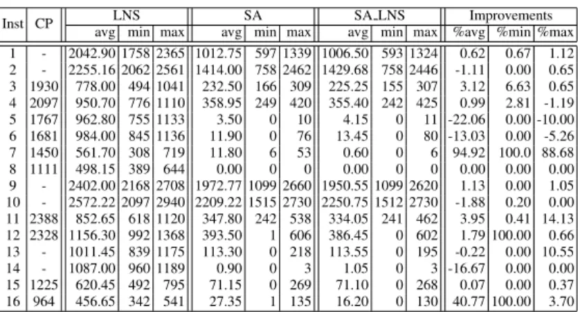
Table 5 reports the cost found by each technique on the 16 instances. LNS, SA and SA LNS were run on 20 different seeds and the average, min and max cost found over the 20 runs are reported. The CP approach is entirely deterministic and a single run is therefore shown. The last three columns show the percentage of improvements given by SA LNS over SA alone. Two computers were used, CP was run on a Mac-Book4within a time limit of 420s and the others were run on an iMac5within a time
4
Mac OS X 10.4.11, 2 GHz Intel Core 2 Duo, 2 GB 667 Mhz DDR2.
limit of 372s6. Firstly, the LNS scheme outperforms CP alone (even by only looking at instances where CP does find a feasible solution) while being a very simple modifi-cation of CP. Secondly, LNS is itself outperformed by the SA. We observed here that it remains stuck in local minima despite the large size of the neighbourhood. [19] out-lines the same problem and suggests that the LNS scheme still needs other and more powerful diversification mechanisms. Finally, SA LNS improves LNS but is not very convincing. The CP moves do not seem to bring much more flexibility to the SA to escape local minima in general. It allows, however, to find three new optimal solutions (instances 7, 12 and 16) and improves significantly the resolution of two instances (7 and 16). Note that all the minimum costs are improved showing that LNS does play a role in the final intensification stage even if this does not give a major improvement.
Table 5.Overall results on 20 runs reporting the average, min and max cost.
Inst CP LNS SA SA LNS Improvements
avg min max avg min max avg min max %avg %min %max 1 - 2042.90 1758 2365 1012.75 597 1339 1006.50 593 1324 0.62 0.67 1.12 2 - 2255.16 2062 2561 1414.00 758 2462 1429.68 758 2446 -1.11 0.00 0.65 3 1930 778.00 494 1041 232.50 166 309 225.25 155 307 3.12 6.63 0.65 4 2097 950.70 776 1110 358.95 249 420 355.40 242 425 0.99 2.81 -1.19 5 1767 962.80 755 1133 3.50 0 10 4.15 0 11 -22.06 0.00 -10.00 6 1681 984.00 845 1136 11.90 0 76 13.45 0 80 -13.03 0.00 -5.26 7 1450 561.70 308 719 11.80 6 53 0.60 0 6 94.92 100.0 88.68 8 1111 498.15 389 644 0.00 0 0 0.00 0 0 0.00 0.00 0.00 9 - 2402.00 2168 2708 1972.77 1099 2660 1950.55 1099 2620 1.13 0.00 1.05 10 - 2572.22 2097 2940 2209.22 1515 2730 2250.75 1512 2730 -1.88 0.20 0.00 11 2388 852.65 618 1120 347.80 242 538 334.05 241 462 3.95 0.41 14.13 12 2328 1156.30 992 1368 393.50 1 606 386.45 0 602 1.79 100.00 0.66 13 - 1011.45 839 1175 113.30 0 218 113.55 0 195 -0.22 0.00 10.55 14 - 1087.00 960 1189 0.90 0 3 1.05 0 3 -16.67 0.00 0.00 15 1225 620.45 492 795 71.15 0 269 71.10 0 268 0.07 0.00 0.37 16 964 456.65 342 541 27.35 1 135 16.20 0 130 40.77 100.00 3.70
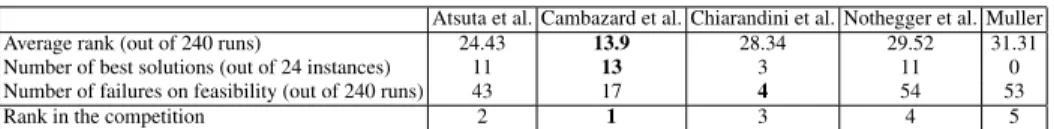
Comparisons with other Algorithms in the Competition. Five algorithms7 were
choosen for the final phase and evaluated on 24 instances (the 16 already mentioned and 8 unknown competition ones). Since all solvers were randomised, 10 runs per in-stance were performed giving 50 runs per inin-stance. Each run was ranked among the 50 for each instance and the average rank across all runs and all instances was used to give a rank to each algorithm. Table 6 shows the ranking of each algorithm, with the number of times they have found the best solution among all runs for a given instance, and the number of times they have failed to find a feasible solution.
Our local search with a score of 13.9 therefore did significantly better than the al-gorithm of Atsuta et al. that came second with 24.43. Our approach appeared generally more robust for both finding feasible and good solutions (Chirandini et al. being the most robust on feasibility only). It also obtained the best results on many instances. It is however very interesting to notice that it was outperformed on instances we considered here as very hard on feasibility for our algorithm, e.g. instance 10. Nothegger et al. or
6Both time limits were established by the benchmarking program used during the competition. 7
The other four algorithms were developped by: M. Atsuta, K. Nonobe, T. Ibaraki; M. Chiaran-dini, C. Fawcett, H. H Hoos; C. Nothegger, A. Mayer, A. Chwatal, G. Raidi; T.Muller.
Table 6.Ranking of the five finalists from the tests ran by the organizers on the 24 instances. Atsuta et al. Cambazard et al. Chiarandini et al. Nothegger et al. Muller Average rank (out of 240 runs) 24.43 13.9 28.34 29.52 31.31 Number of best solutions (out of 24 instances) 11 13 3 11 0 Number of failures on feasibility (out of 240 runs) 43 17 4 54 53
Rank in the competition 2 1 3 4 5
Atsuki et al. could not only systematically find a feasible solution on instance 10 but also the optimal one. On the other hand, these algorithms fail to find feasible solutions on instances where our approach succeeds easily. On instance 9 they only find a feasible solution 30% of the time but when they do, it is the optimal one. This lead us to con-jecture that they have been using the soft cost to guide the search of feasible solutions. On very tight instances, this strategy pays off as there are maybe few feasible solutions and it is known that an optimal solution of cost 0 always exists. On other instances it either misleads the search or just slows down the process, thus degrading the results. This shows that there is a significant room for improvement in our results.
8
Conclusion
We have presented a comprehensive study of a university timetabling problem, com-paring a variety of local search and constraint programming approaches. We designed a constraint programming approach that proceeds by decomposing the list-colouring and the matching subproblems and outperforms more classical CP models. Lower bounds were introduced to tackle soft constraints, leading to the first complete algorithm for this problem. While our local search technique benefits from the experience of the 2003 competition, we have presented several improvements to deal with hard constraints; the results show more maturity than the CP technique. However, an LNS scheme inte-grating both our CP and LS approaches obtained the best results. The structure of the list-colouring graph made of large and overlapping cliques was shown to be important for both CP and LS techniques. Improving the propagation we can achieve from a col-lection of ALLDIFF constraints is very important in this context. Arc-consistency on two overlapping ALLDIFFis already known to be NP-Complete [3] but a number of pragmatic filtering rules could be designed. This is an important topic for future work.
References
1. S. Abdullah, E. K. Burke, and B. McCollum. Using a randomised iterative improvement algorithm with composite neighbourhood structures for course timetabling. InMIC 05: The 6th Meta-Heuristic International Conference, 2005.
2. A. Aggoun and N. Beldiceanu. Extending chip in order to solve complex scheduling and placement problems.Mathematical Computing and Modelling, 17(7):57–73, 1993.
3. N. Beldiceanu, M. Carlsson, S. Demassey, and T. Petit. Global constraint catalogue: Past, present and future.Constraints, 12(1):21–62, 2007.
4. H. Cambazard, P.E. Hladik, A.M. D´eplanche, N. Jussien, and Y. Trinquet. Decomposition and learning for a real time task allocation problem. InProc. of CP, pages 153–167, 2004. 5. M. W. Carter and G. Laporte. Recent developments in practical course timetabling. InPATAT,
6. M. Chiarandini, M. Birattari, K. Socha, and O. Rossi-Doria. An effective hybrid algorithm for university course timetabling.J. Scheduling, 9(5):403–432, 2006.
7. E. Danna and L. Perron. Structured vs. unstructured large neighborhood search: A case study on job-shop scheduling problems with earliness and tardiness costs. InCP, pages 817–821, 2003.
8. J.L. de Siqueira and J.F. Puget. Explanation-based generalisation of failures. InEuropean Conference on Artificial Intelligence (ECAI’88), pages 339–344, 1988.
9. D. de Werra. An introduction to timetabling. European Journal of Operational Research, 19(2):151–162, February 1985.
10. L. Di Gaspero and A. Schaerf. Neighborhood portfolio approach for local search applied to timetabling problems.Journal of Mathematical Modeling and Algorithms, 5(1):65–89, 2006. 11. P. Galinier and A. Hertz. A survey of local search methods for graph coloring. Comput.
Oper. Res., 33(9):2547–2562, 2006.
12. J.N. Hooker and G. Ottosson. Logic-based benders decomposition.Mathematical Program-ming, 96:33–60, 2003.
13. V. Jain and I. E. Grossmann. Algorithms for hybrid milp/cp models for a class of optimization problems.INFORMS Journal on Computing, 13:258–276, 2001.
14. S. Kirkpatrick, C. D. Gelatt, and M. P. Vecchi. Optimization by simulated annealing.Science, Number 4598, 13 May 1983, 220, 4598:671–680, 1983.
15. P. Kostuch. The university course timetabling problem with a three-phase approach. In
PATAT, pages 109–125, 2004.
16. H. W. Kuhn. The hungarian method for the assignment problem. Naval Research Logistics Quarterly, 2(1):83–98, 1955.
17. R. Lewis, B. Paechter, and B. McCollum. Post enrolment based course timetabling: A de-scription of the problem model used for track two of the second international timetabling competition. Technical report, Cardiff University, 2007.
18. M. W. Moskewicz, C. F. Madigan, Y. Zhao, L. Zhang, and S. Malik. Chaff: Engineering an Efficient SAT Solver. InProceedings of the 38th Design Automation Conference (DAC’01), pages 530– 535, 2001.
19. L. Perron and P. Shaw. Combining forces to solve the car sequencing problem. InCPAIOR, pages 225–239, 2004.
20. L. Perron, P. Shaw, and V. Furnon. Propagation guided large neighborhood search. InCP, pages 468–481, 2004.
21. P. Refalo. Impact-based search strategies for constraint programming. InCP, pages 557–571, 2004.
22. J.C. R´egin. A filtering algorithm for constraints of difference in CSPs. InProceedings of the 12th National Conference on Artificial Intelligence (AAAI-94), pages 362–367, 1994. 23. J.C. R´egin. Generalized arc consistency for global cardinality constraint. InNational
Con-ference on Artificial Intelligence (AAAI’96), pages 209–215, 1996.
24. O. Rossi-Doria, M. Sampels, M. Birattari, M. Chiarandini, M. Dorigo, L. M. Gambardella, J. D. Knowles, M. Manfrin, M. Mastrolilli, B. Paechter, L. Paquete, and T. St¨utzle. A com-parison of the performance of different metaheuristics on the timetabling problem. InPATAT, pages 329–354, 2002.
25. N. Sadeh and M.S. Fox. Variable and Value Ordering Heuristics for the Job-Shop Scheduling Constraint Satisfaction Problem.Artificial Intelligence, 86(1):1–41, September 1996. 26. A. Schaerf. A survey of automated timetabling.Artificial Intelligence Review, 13(2):87–127,
1999.
27. P. Shaw. Using constraint programming and local search methods to solve vehicle routing problems. InCP, pages 417–431, 1998.