Methods
for Big Data Optimization
Doctoral thesis
Martin Tak´
aˇ
c
Supervisor:
Dr. Peter Richt´
arik
Doctor of Philosophy
The University of Edinburgh
Randomized Coordinate Descent
Methods
for Big Data Optimization
Doctoral thesis
Martin Tak´
aˇ
c
School of Mathematics
The University of Edinburgh
Supervisor:
Dr. Peter Richt´
arik
Edinburgh 2014
Randomized Coordinate Descent Methods
for Big Data Optimization
Martin Tak´aˇc
E-mail: [email protected]
Website: http: // mtakac. com
Dr. Peter Richt´arik
E-mail: [email protected]
Website: http: // www. maths. ed. ac. uk/ ~ prichtar
School of Mathematics The University of Edinburgh James Clerk Maxwell Building The King’s Buildings
Mayfield Road Edinburgh
Scotland EH9 3JZ
c
2014 Martin Tak´aˇc Doctoral thesis
Compilation date: April 27, 2014 Typeset in LATEX
son Martin
and everybody I love.
The candidate confirms that the work submitted is his own, except where work which has formed part of jointly-authored publications has been included. The contribution of the candidate and the others authors to this work has been explicitly indicated below. The candidate confirms that appropriate credit has been given within the thesis where reference has been made to the work of others.
The table below indicates which chapters are based on a work from jointly-authored publi-cations. The candidate contributed to every result of all papers this thesis is based on.
Chapter 1 2 3 4 5
Ref. [53, 54, 55] [53] [54, 56] [55] [66]
(Martin Tak´aˇc, April 27, 2014)
God gave you a gift of 86,400 seconds today. Have you used one to say ’thank you?’
— William Arthur Ward (1921–1994) I would like to express my special appreciation and thanks to my advisor Dr. Peter Richt´arik. Peter, you have been a tremendous mentor for me! You have shown the attitude and the substance of a genius: you continually and persuasively conveyed a spirit of adventure in regard to the research. You were constantly encouraging my research and also allowed me to grow as a research scientist. You taught me how to deliver the best talk, you advised me how to prepare the perfect slides, you have spent so much time listening to my practice talks, suggesting improvements and offering career advice. All you did for me, it has all been priceless. With you research was, indeed, fun and a joy and hence it has become almost a leisure activity!
I would like to thank my second supervisor Professor Jacek Gondzio, for his helpfulness and willingness to chat about research. Your advice was very helpful in my formation as a scientist.
Now, I would like to thank several people:
• I also want to say big “Thank you!” to doc. Dr. Milan Hamala, Professor Daniel ˇSevˇcoviˇc, Professor Pavel Brunovsk´y and doc. Dr. Margar´eta Halick´a, who initiated and helped to grow my desire in optimization and research in general. I am sure that without them, I wouldn’t have started on the academic career-path. Your support and constant interest in my progress and achievements during my PhD study were very encouraging!
• I am also very grateful to many researchers I had the chance to collaborate with. Espe-cially to Professor Yurii Nesterov, Professor Fran¸cois Glineur, Professor Nathan Srebro,
Dr. Selin Damla Ahipa¸sao˘glu, Dr. Ngai-Man Cheung, Dr. Olivier Devolder, Dr. Jakub Mareˇcek and Avleen Bijral.
• I feel indebted to Dr. Rachael Tappenden for many interesting chats, research collabo-rations, minisymposia co-organization and all the time she spent with proofreading my slides and papers! Thank you Rachael, your help was extremely useful and constructive. You were always willing to help with everything.
• I am filled with gratitude for many interesting discussions and chats with researchers including Professor Stephen Wright, Professor Michael J. D. Powell, Professor Roger Fletcher, Dr. Michel Baes and to all of my colleagues including Professor Jared Tanner, Dr. Coralia Cartis, Dr. Andreas Grothey, Dr. Julian Hall, Professor Ken McKinnon, Dr. Martin Lotz, Dr. Pavel G. Zhlobich and Kimonas Fountoulakis for many interesting talks and ideas.
I am grateful for all the financial support I got, especially from the Centre for Numerical Algorithms and Intelligent Software (funded by EPSRC grant EP/G036136/1) and Scottish Funding Council. I have been also supported by following grants: EPSRC grants EP/J020567/1 (Algorithms for Data Simplicity), EP/I017127/1 (Mathematics for Vast Digital Resources) and EPSRC First Grant EP/K02325X/1 (Accelerated Coordinate Descent Methods for Big Data Problems).
Furthermore, I would also like to thank my parents for their endless love and support. Finally, and most importantly to me, I would like to express appreciation to my beloved wife PharmDr. M´aria Tak´aˇcov´a who spent many sleepless nights (especially when I was travelling far from home) and was always my support in the moments when there was no one to answer my queries. My love, I am sure, I would not have made it thus far! Your help, support, and your faith in me was the fuel which makes me go. I will be grateful forever for your love. Thank you!
The universe is governed by science. But science tells us that we can’t solve the equations, directly in the abstract.
— Stephen Hawking (1942) This thesis consists of 5 chapters. We develop new serial (Chapter 2), parallel (Chapter 3), distributed (Chapter 4) and primal-dual (Chapter 5) stochastic (randomized) coordinate descent methods, analyze their complexity and conduct numerical experiments on synthetic and real data of huge sizes (GBs/TBs of data, millions/billions of variables).
In Chapter 2 we develop a randomized coordinate descent method for minimizing the sum of a smooth and a simple nonsmooth separable convex function and prove that it obtains an -accurate solution with probability at least 1−ρin at most O((n/) log(1/ρ)) iterations, where n is the number of blocks. This extends recent results of Nesterov [43], which cover the smooth case, to composite minimization, while at the same time improving the complexity by the factor of 4 and removing from the logarithmic term. More importantly, in contrast with the aforementioned work in which the author achieves the results by applying the method to a regularized version of the objective function with an unknown scaling factor, we show that this is not necessary, thus achieving first true iteration complexity bounds. For strongly convex functions the method converges linearly. In the smooth case we also allow for arbitrary probability vectors and non-Euclidean norms. Our analysis is also much simpler.
In Chapter 3 we show that the randomized coordinate descent method developed in Chapter 2 can be accelerated by parallelization. The speedup, as compared to the serial method, and referring to the number of iterations needed to approximately solve the problem with high probability, is equal to the product of the number of processors and a natural and easily
computable measure of separability of the smooth component of the objective function. In the worst case, when no degree of separability is present, there is no speedup; in the best case, when the problem is separable, the speedup is equal to the number of processors. Our analysis also works in the mode when the number of coordinates being updated at each iteration is random, which allows for modeling situations with variable (busy or unreliable) number of processors. We demonstrate numerically that the algorithm is able to solve huge-scale`1-regularized least
squares problems with a billion variables.
In Chapter 4 we extended coordinate descent into a distributed environment. We initially partition the coordinates (features or examples, based on the problem formulation) and assign each partition to a different node of a cluster. At every iteration, each node picks a random subset of the coordinates from those it owns, independently from the other computers, and in parallel computes and applies updates to the selected coordinates based on a simple closed-form closed-formula. We give bounds on the number of iterations sufficient to approximately solve the problem with high probability, and show how it depends on the data and on the partitioning. We perform numerical experiments with a LASSO instance described by a 3TB matrix.
Finally, in Chapter 5, we address the issue of using mini-batches in stochastic optimization of Support Vector Machines (SVMs). We show that the same quantity, the spectral norm of the data, controls the parallelization speedup obtained for both primal stochastic subgradient descent (SGD) and stochastic dual coordinate ascent (SCDA) methods and use it to derive novel variants of mini-batched (parallel) SDCA. Our guarantees for both methods are expressed in terms of the original nonsmooth primal problem based on the hinge-loss.
Our results in Chapters 2 and 3 are cast for blocks (groups of coordinates) instead of coordinates, and hence the methods are better described asblock coordinate descent methods. While the results in Chapters 4 and 5 are not formulated for blocks, they can be extended to this setting.
List of Tables xii
List of Figures xiii
List of Algorithms xiv
1 Introduction 1
1.1 Optimization . . . 1
1.2 Stochastic Block Coordinate Descent Methods . . . 3
1.3 A Brief Overview of the Thesis . . . 5
1.4 The Optimization Problem . . . 6
1.5 Notation and Assumptions . . . 7
1.5.1 Block Structure . . . 7
1.5.2 Global Structure . . . 8
1.5.3 Smoothness off . . . 8
1.5.4 Separability of Ψ . . . 9
1.5.5 Strong Convexity ofF . . . 9
1.5.6 Level Set Radius . . . 10
1.5.7 Projection Onto a Set of Blocks . . . 10
1.6 Key Technical Tool For High Probability Results . . . 11
2 Serial Coordinate Descent Method 14 2.1 Literature Review . . . 14
2.2 The Algorithm . . . 15
2.3 Summary of Contributions . . . 16
2.4 Iteration Complexity for Composite Functions . . . 18
2.4.1 Convex Objective . . . 20
2.4.2 Strongly Convex Objective . . . 21
2.4.3 A Regularization Technique . . . 23
2.5 Iteration Complexity for Smooth Functions . . . 25
2.5.1 Convex Objective . . . 26
2.5.2 Strongly Convex Objective . . . 28
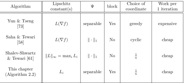
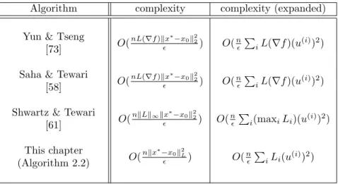
2.6 Comparison of CD Methods with Complexity Guarantees . . . 29
2.6.1 Smooth Case (Ψ = 0) . . . 29
2.6.2 Nonsmooth Case (Ψ6= 0) . . . 31
2.7 Numerical Experiments . . . 32
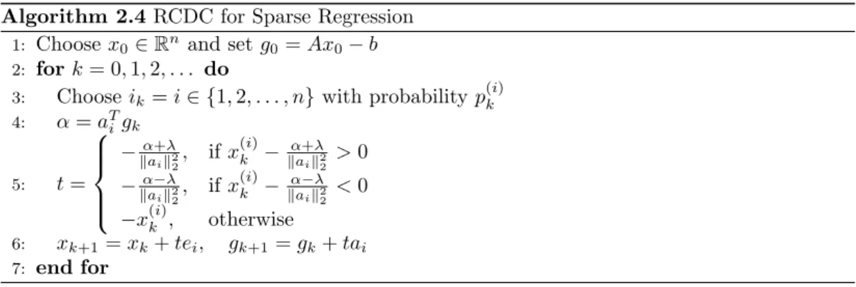
2.7.1 Sparse Regression / Lasso . . . 32
2.7.2 Linear Support Vector Machines . . . 40
3 Parallel Coordinate Descent Method 44 3.1 Literature review . . . 46 3.2 Contents . . . 47 3.3 The Algorithm . . . 47 3.4 Summary of Contributions . . . 50 3.5 Block Samplings . . . 54
3.5.1 Uniform, Doubly Uniform and Nonoverlapping Uniform Samplings . . . . 54
3.5.2 Technical Results . . . 57
3.6 Expected Separable Overapproximation . . . 60
3.6.1 Deterministic Separable Overapproximation (DSO) of Partially Separable Functions . . . 62
3.6.2 ESO for a Convex Combination of Samplings . . . 64
3.6.3 ESO for a Conic Combination of Functions . . . 66
3.7 Expected Separable Overapproximation (ESO) of Partially Separable Functions . 67 3.7.1 Uniform Samplings . . . 67
3.7.2 Nonoverlapping Uniform Samplings . . . 69
3.7.3 Nice Samplings . . . 70
3.7.4 Doubly Uniform Samplings . . . 71
3.8 Iteration Complexity . . . 72
3.8.1 Convex Case . . . 73
3.8.2 Strongly Convex Case . . . 76
3.9 Optimal Probabilities in the Smooth Case . . . 77
3.9.1 Analysis . . . 78
3.9.2 Nonuniform Samplings and ESO . . . 80
3.9.3 Optimal Probabilities . . . 81
3.10 Numerical Experiments . . . 82
3.10.1 A LASSO Problem with 1 Billion Variables . . . 83
3.10.2 Theory Versus Reality . . . 86
3.10.3 Training Linear SVMs with Bad Data for PCDM . . . 87
3.10.4 L2-regularized Logistic Regression with Good Data for PCDM . . . 90
3.10.5 Optimal Probabilities . . . 91
4 Distributed Coordinate Descent Method 93 4.1 The Algorithm . . . 95
4.2 Iteration Complexity . . . 97
4.2.1 Four Important Quantities: σ0, ω0, σ, ω . . . 97
4.2.2 Choice of the Stepsize Parameterβ . . . 100
4.2.3 Expected Separable Approximation . . . 101
4.2.4 Fast Rates for Distributed Learning with Hydra . . . 103
4.3 Discussion . . . 104
4.3.1 Insights Into the Convergence Rate . . . 104
4.3.2 Comparison with Other Methods . . . 106
4.4 Distributed Computation of the Gradient . . . 107
4.4.1 Basic Protocol . . . 108
4.4.2 Advanced Protocols . . . 108
4.5 Experiments . . . 110
4.5.1 Performance of Communication Protocols . . . 110
5 Primal-Dual Coordinate Descent Method 113 5.1 Introduction . . . 113
5.2 Related Work . . . 114
5.3 Support Vector Machines . . . 115
5.4 Mini-Batches in Primal Stochastic Gradient Descent Methods . . . 116
5.5 Mini-Batches in Dual Stochastic Coordinate Ascent Methods . . . 120
5.5.1 Naive Mini-Batching . . . 121
5.5.3 Aggressive Mini-Batching . . . 124
5.6 Experiments . . . 125
5.7 Summary and Discussion . . . 126
5.8 Proof of Theorem 24 . . . 129
Bibliography 134 A Notation Glossary 139 A.1 Notation Introduced in Chapter 1 . . . 139
A.2 Notation Introduced in Chapter 2 . . . 140
A.3 Notation Introduced in Chapter 3 . . . 140
A.4 Notation Introduced in Chapter 4 . . . 140
2.1 Summary of complexity results obtained in this chapter. . . 17
2.2 Comparison of our results to the results in [43]. . . 30
2.3 Comparison of CD approaches for minimizing composite functions. . . 31
2.4 Comparison of iteration complexities of the methods listed in Table 2.3. . . 32
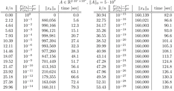
2.5 Comparison of solving time as a function ofkx∗k 0. . . 33
2.6 Performance of UCDC on a sparse regression instance with a million variables. . . . 34
2.7 Performance of UCDC on a sparse regression instance with a billion variables. . . 35
2.8 UCDC needs many more iterations whenm < n, but local convergence is still fast. . 35
2.9 A list of a few popular loss functions. . . 41
2.10 Lipschitz constants and coordinate derivatives for SVM. . . 41
2.11 Cross validation accuracy (CV-A) and testing accuracy (TA) for various choices ofγ. 42 3.1 Three examples of loss of functions. . . 46
3.2 Summary of the main complexity results for PCDM established in this chapter. . . . 50
3.3 New and known gradient methods obtained as special cases of our general framework. 51 3.4 Values of parametersβ and wfor various samplings ˆS. . . 52
3.5 Parallelization speedup factors for DU samplings. . . 75
3.6 A LASSO problem with 109 variables solved by PCDM1 withτ= 1, 2, 4, 8, 16 and 24. . . 84
3.7 PCDM accelerates linearly inτ on a good dataset. . . 91
4.1 Stepsize parameterβ =β∗ for several special cases of Hydra. . . 105
4.2 Information needed in Step 6 of Hydra. . . 107
4.3 Duration of a single Hydra iteration for 3 communication protocols. . . 111
5.1 Datasets and regularization parametersλused in experiments. . . 126
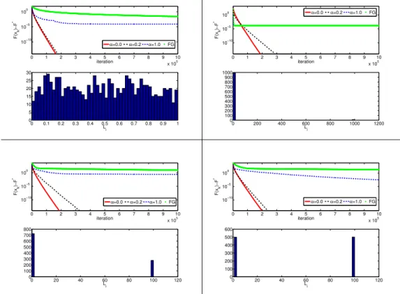
2.1 Development ofF(xk)−F∗ for sparse regression problem. . . 36
2.2 Comparison of RCDC. . . 37
2.3 Development of non-zero elements in xk through iterations. . . 39
2.4 Comparison of different shrinking strategies. . . 40
2.5 Evolution of a tested accuracy. . . 42
3.1 Parallelization speedup factor. . . 76
3.2 Histogram of the cardinalities of the rows ofA. . . 83
3.3 Four computational insights into the workings of PCDM1. . . 86
3.4 Theoretical speedup factor vs. experiment. . . 87
3.5 PCDM on the rcv1 dataset. . . 89
3.6 PCDM accelerates well with more processors on a dataset with smallω. . . 90
3.7 Comparison of optimal method vs. uniform and fully parallel. . . 91
4.1 In terms of the number of iterations, very little is lost by usingc >1 as opposed to c= 1. . . 106
4.2 Parallel-serial (PS; left) vs Fully Parallel (FP; right) approach. . . 109
4.3 ASL protocol with c= 4 nodes. . . 109
4.4 Evolution of F(xk)−F∗ in time. . . 112
5.1 Number of iterations needed to find a 0.001-accurate primal solution. . . 127
5.2 Evolutions of primal and dual sub-optimality and test error. . . 128
2.1 RCDC(p, x0) (RandomizedCoordinateDescent for Composite Functions) . . . . 16
2.2 UCDC(x0) (UniformCoordinateDescent for Composite Functions) . . . 18
2.3 RCDS(p, x0) (RandomizedCoordinateDescent forSmooth Functions) . . . 26
2.4 RCDC for Sparse Regression . . . 33
3.1 PCDM1 (ParallelCoordinateDescentMethod 1) . . . 47
3.2 PCDM2 (ParallelCoordinateDescentMethod 2) . . . 48
3.3 ‘NSync: Nonuniform SYNchronous Coordinate descent . . . 78
4.1 Hydra (HYbriD cooRdinAte descent) . . . 96
5.1 Pegasos with Mini-Batches . . . 117
5.2 SDCA with Mini-Batches (aggressive) . . . 125
1
Introduction
I have not failed. I’ve just found 10,000 ways that won’t work.
— Thomas Alva Edison (1847-1931)
1.1
Optimization
In mathematics, optimization is the process of selecting the best decision x∗ from a set of available (feasible) decisions. We can associate with every admissible (feasible) decisionx∈X
a real-valued functionF(x) which measures the quality ofx(lower values correspond to better decisions). Optimization thus seeks to find a minimizer of F on X. The problem of finding the exact minimizer can be very hard (maybe due to the size or structureof the function F, or the exact solution may not be obtainable in a closed form). In practice, an approximate solutionx (whereF(x)≤F(x∗) +) is sufficient, where is our target approximation level.
The choice of is problem specific. In many machine learning problems,= 10−2can already
be sufficient. The approximate solution can be obtained by an iterative process (optimization algorithm), where we start with some starting solution and then in each iteration find a new solution with better quality (lower function value).
Big data optimization. Recently there has been a surge in interest in the design of al-gorithms suitable for solving convex optimization problems with a huge number of variables [53, 44]. Indeed, the size of problems arising in fields such as machine learning [5], network analysis [85], PDEs [79], truss topology design [52] and compressed sensing [26] usually grows with our capacity to solve them, and is projected to grow dramatically in the next decade. In
fact, much of computational science is currently facing the “big data” challenge, and this work is aimed at developing optimization algorithms suitable for the task.
Our goals. The goal of this thesis, in the broadest sense, is to develop efficient methods for solving structured convex optimization problems with some or all of these (not necessarily distinct) properties:
1. Size of Data. The size of the problem, measured as the dimension of the variable of interest, is so large that the computation of a single function value or gradient is prohibitive. There are several situations in which this is the case, let us mention two of them.
• Memory. If the dimension of the space of variables is larger than the available memory, the task of forming a gradient or even of evaluating the function value may be impossible to execute and hence the usual gradient methods will not work.
• Patience. Even if the memory does not preclude the possibility of taking a gra-dient step, for large enough problems this step will take considerable time and, in some applications such as image processing, users might prefer to see/have some intermediary results before a single iteration is over.
2. Nature of Data. The nature and structure of data describing the problem may be an obstacle in using current methods for various reasons, including the following.
• Completeness. If the data describing the problem is not immediately available in its entirety, but instead arrives incomplete in pieces and blocks over time, with each block “corresponding to” one variable, it may not be realistic (for various reasons such as “memory” and “patience” described above) to wait for the entire data set to arrive before the optimization process is started.
• Source. If the data is distributed on a network not all nodes of which are equally responsive or functioning, it may be necessary to work with whatever data is available at a given time.
It appears that a very reasonable approach to solving some problems characterized above is to use(block) coordinate descent methods (CD). In this thesis we design new serial, parallel, distributed and primal-dual stochastic (block) coordinate descent methods.
1.2
Stochastic Block Coordinate Descent Methods
The basic algorithmic strategy of CD methods is known in the literature under various names such as alternating minimization, coordinate relaxation, linear and non-linear Gauss-Seidel methods, subspace correction and domain decomposition. As working with all the variables of an optimization problem at each iteration may be inconvenient, difficult or impossible for any or all of the reasons mentioned above, the variables are partitioned into manageable blocks, with each iteration focused on updating a single block only, the remaining blocks being fixed. Both for their conceptual and algorithmic simplicity, CD methods were among the first optimization approaches proposed and studied in the literature (see [2] and the references therein; for a survey of block CD methods in semidefinite programming we refer the reader to [75]). While they seem to have never belonged to the mainstream focus of the optimization community, a renewed interest in CD methods was sparked recently by their successful application in several areas—training support vector machines in machine learning [7, 4], [61], [82], [81], optimization [31, 35, 34, 45, 36, 37, 46, 25, 22, 28, 74, 72, 84, 58, 43, 76], compressed sensing [26], regression [78], protein loop closure [6] and truss topology design [52]—partly due to a change in thesize
andnature of datadescribed above.
Order of coordinates. Efficiency of a CD method will necessarily depend on the balance between time spent on choosing the block to be updated in the current iteration and the quality of this choice in terms of function value decrease. One extreme possibility is a greedy
strategy in which the block with the largest descent or guaranteed descent is chosen. In our setup such a strategy is prohibitive as i) it would require all data to be available and ii) the work involved would be excessive due to the size of the problem. Even if one is able to compute all partial derivatives, it seems better to then take a full gradient step instead of a coordinate one, and avoid throwing almost all of the computed information away. On the other end of the spectrum are two very cheap strategies for choosing the incumbent coordinate: cyclic and
random. Surprisingly, it appears that complexity analysis of a cyclic CD method in satisfying generality has not yet been done. The only attempt known to us is the work of Saha and Tewari [58]; the authors consider the case of minimizing a smooth convex function and proceed by establishing a sequence of comparison theorems between the iterates of their method and the iterates of a simple gradient method. Their result requires an isotonicity assumption1. Note
that a cyclic strategy assumes that the data describing the next block is available when needed which may not always be realistic. The situation with a random strategy seems better; here
1A functionF :
are some of the reasons:
(i) Recent efforts suggest that complexity results are perhaps more readily obtained for ran-domized methods and that randomization can actually improve the convergence rate [65], [23], [61].
(ii) Choosing all blocks with equal probabilities should, intuitively, lead to similar results as is the case with a cyclic strategy. In fact, a randomized strategy is able to avoid worst-case order of coordinates, and hence might be preferable.
(iii) Randomized choice seems more suitable in cases when not all data is available at all times.2
(iv) One may study the possibility of choosing blocks with different probabilities (we do this in Section 2.5). The goal of such a strategy may be either to improve the speed of the method (in Section 2.7.1 we introduce a speedup heuristic based on adaptively changing the probabilities), or a more realistic modeling of the availability frequencies of the data defining each block.
Step size. Once a coordinate (or a block of coordinates) is chosen to be updated in the current iteration, partial derivative can be used to drive the steplength in the same way as it is done in the usual gradient methods. As it is sometimes the case that the computation of a partial derivative is much cheaper and less memory demanding than the computation of the entire gradient, CD methods seem to be promising candidates for problems described above. It is important that line search, if any is implemented, is very efficient. The entire data set is either huge or not available and hence it is not reasonable to use function values at any point in the algorithm, including the line search. Instead, cheap partial derivative and other information derived from the problem structure should be used to drive such a method.
Coordinate descent methods. Coordinate descent methods (CDM) are one of the most successful classes of algorithms in the big data optimization domain. Broadly speaking, CDMs are based on the strategy of updating a single coordinate (or a single block of coordinates) of the vector of variables at each iteration. This often drastically reduces memory requirements as well as the arithmetic complexity of a single iteration, making the methods easily implementable and 2If data were not available in memory and one would like to follow, e.g., cyclic order or greedy selection
of coordinates, then one would have to wait until the required data are fetched from a source. In contrast, in many applications with streaming data, e.g., involving on-line support vector machine (SVM), one may plausibly assume that the stream of in-coming data is sufficiently random to see a sequential choice of from the stream as a random selection.
scalable. In certain applications, a single iteration can amount to as few as 4 multiplications and additions only [52]! On the other hand, many more iterations are necessary for convergence than it is usual for classical gradient methods. Indeed, the number of iterations a CDM requires to solve a smooth convex optimization problem isO(nLR˜ 2
), whereis the error tolerance,nis
the number variables (or blocks of variables), ˜Lis the average of the Lipschitz constants of the gradient of the objective function associated with the variables (blocks of variables) andR is the distance from the starting iterate to the set of optimal solutions. On balance, as observed by numerous authors, serial CDMs are much more efficient for big data optimization problems than most other competing approaches, such as gradient methods [43, 52].
Parallelization. We wish to point out that for truly huge-scale problems it is absolutely nec-essary toparallelize. This is in line with the rise and ever increasing availability of high perfor-mance computing systems built around multi-core processors, GPU-accelerators and computer clusters, the success of which is rooted in massive parallelization. This simple observation, combined with the remarkable scalability of serial CDMs, leads to our belief that the study of parallel coordinate descent methods (PCDMs) is a very timely topic.
1.3
A Brief Overview of the Thesis
Section 1.4 introduces the main problem we deal with in the whole thesis. Then the basic nota-tion which is shared in all other chapters is introduced. Afterwards, we state one very important technical result (Theorem 1) which will be used to derive all high probability convergence re-sults in this thesis. Chapter 2 introduces the generic serial coordinate descent algorithm and analyzes its convergence for both its uniform and nonuniform variant. In Chapter 3 we develop parallel variants of the methods, the analysis of which depends on the notion of ESO, which is a novel technical tool developed in [54]. This ESO concept enables us to analyze parallel coordinate descent algorithms (PCDM) and derive iteration complexity results. It turns out that ESO is so powerful that also allows us to analyze a distributed modification of PCDM, which we call Hydra, in Chapter 4. In Chapter 5 we focus on the problem of optimization of Support Vector Machines (SVMs). We apply the ESO concept and show that the paralleliza-tion speedup obtained for both primal stochastic subgradient descent (SGD) and stochastic dual coordinate ascent (SCDA) is driven by the same quantity, which depends on the spectral norm of the data. Our mini-batch SDCA method is the first parallel primal-dual coordinate descent method in the literature.
1.4
The Optimization Problem
In this thesis we study theiteration complexityof randomized block coordinate descent methods applied to the problem of minimizing acomposite objective function, i.e., a function formed as the sum of a smooth convex and a simple nonsmooth convex term:
min
x∈RN
F(x)def= f(x) + Ψ(x). (1.1)
We assume that this problem has a minimum (F∗ >−∞),f has (block) coordinate Lipschitz continuous gradient, and Ψ is a (block) separable proper closed convex extended real valued function (block separability will be defined precisely in Section 1.5). Possible choices of Ψ include:
(i) Ψ≡0. This covers the case ofsmooth minimizationand was considered in [43]. (ii) Ψ is the indicator function of a block-separable convex set (a box), i.e.,
Ψ(x) =IS1×···×Sn(x) def = 0 if x(i)∈S i ∀i, +∞ otherwise, wherex(i)is blockiofx∈
RN (to be defined precisely in Section 1.5) andS1, . . . , Sn are
closed convex sets. This choice of Ψ models problems with smooth objective and convex constraints on blocks of variables. Indeed, (1.1) takes on the form
min f(x) subject to x(i)∈Si, i= 1, . . . , n.
Iteration complexity results in this case were given in [43].
(iii) Ψ(x)≡λkxk1forλ >0. In this case we decomposeRN intoN blocks, each correspond-ing to one coordinate of x. Increasing λ encourages the solution of (1.1) to be sparser [77]. Applications abound in, for instance, machine learning [7], statistics [71] and signal processing [26]. The first iteration complexity results for the case with a single block were given in [42].
(iv) There are many more choices such as the elastic net [87], group lasso [83], [32], [48] and sparse group lasso [18]. One may combine indicator functions with other block separable functions such as Ψ(x) = λkxk1+IS1×···×Sn(x), Si = [li, ui], where the sets introduce
1.5
Notation and Assumptions
Some elements of the setup described in this section was initially used in the analysis of block coordinate descent methods by Nesterov [43] (e.g., block structure, weighted norms and block Lipschitz constants).
1.5.1
Block Structure
The block structure of (1.1) is given by a decomposition of RN into n subspaces as follows.
Let U ∈ RN×N be a column permutation3 of the N ×N identity matrix and further let U = [U1, U2, . . . , Un] be a decomposition ofU intonsubmatrices, withUi being of sizeN×Ni,
whereP
iNi=N.
Proposition 1(Block decomposition4). Any vector x∈
RN can be written uniquely as
x= n X i=1 Uix(i), (1.2) wherex(i)∈RNi. Moreover, x(i)=UT i x.
Proof. Noting thatU UT =P
iUiU T
i is theN ×N identity matrix, we havex=
P
iUiU T i x.
Let us now show uniqueness. Assume thatx=P
iUix (i) 1 = P iUix (i) 2 , where x (i) 1 , x (i) 2 ∈RNi. Since UjTUi= Nj×Nj identity matrix, ifi=j,
Nj×Ni zero matrix, otherwise,
(1.3)
for everyj we get 0 =UT
j (x−x) =UjT P iUi(x (i) 1 −x (i) 2 ) =x (j) 1 −x (j) 2 .
In view of the above proposition, from now on we writex(i) def= UiTx∈RNi, and refer tox(i)
as the i-th blockofx. The definition of partial separability in the introduction is with respect to these blocks. For simplicity, we will sometimes writex= (x(1), . . . , x(n)).
Example 1. Letn=N,Ni= 1for alli andU = [e1, e2, . . . , en]be then×nidentity matrix.
ThenUi =ei is thei-th unit vector andx(i)=eTix∈Ri =R is thei-th coordinate of x. Also,
x=P
ieix
(i).
3The reason why we work with apermutationof the identity matrix, rather than with the identity itself, as
in [43], is to enable the blocks being formed bynonconsecutivecoordinates ofx. This way we establish notation which makes it possible to work with (i.e., analyze the properties of) multiple block decompositions, for the sake of picking the best one, subject to some criteria. Moreover, in some applications the coordinates ofxhave a natural ordering to which the natural or efficient block structure does not correspond.
4This is a straightforeard result; we do not claim any novelty and include it solely for the benefit of the
1.5.2
Global Structure
Inner products. The standard Euclidean inner product in spacesRN and
RNi,i∈[n], will be denoted by h·,·i and [n] will denote a set{1,2, . . . , n}. Letting x, y∈RN, the relationship between these inner products is given by
hx, yi(1.2)= h n X j=1 Ujx(j), n X i=1 Uiy(i)i= n X j=1 n X i=1 hUT i Ujx(j), y(i)i (1.3) = n X i=1 hx(i), y(i)i.
For anyw∈Rn andx, y∈RN we further define
hx, yiw def = n X i=1 wihx(i), y(i)i. (1.4)
For vectorsz= (z1, . . . , zn)T ∈Rnandw= (w1, . . . , wn)T ∈Rnwe writewzdef= (w1z1, . . . , wnzn)T
and foru∈Rn++ we defineu−1 def= (1/u1, . . . ,1/un)T.
Norms. SpacesRNi,i∈[n], are equipped with a pair of conjugate norms: ktk
(i) def
=hBit, ti1/2,
where Bi is an Ni×Ni positive definite matrix andktk∗(i)
def
= maxksk(i)≤1hs, ti=hB
−1
i t, ti1/2,
t∈RNi. Forw∈Rn++, define a pair of conjugate norms inRN by
kxkw= " n X i=1 wikx(i)k2(i) #1/2 , kyk∗w def = max kxkw≤1 hy, xi= " n X i=1 w−i 1(ky(i)k∗ (i)) 2 #1/2 . (1.5)
Note that these norms are induced by the inner product (1.4) and the matricesB1, . . . , Bn. For
a vectorwwe will define a diagonal matrixW = diag(w1, . . . , wn) and we write tr(W) =Piwi.
Often we will use w = L def= (L1, L2, . . . , Ln)T ∈ Rn, where the constants Li are defined
below.
1.5.3
Smoothness of
f
We assume throughout the thesis that the gradient of f is block coordinate-wise Lipschitz continuous, uniformly in x, with positive constants L1, . . . , Ln, i.e., that for all x∈ RN, i = 1,2, . . . , nandt∈Ri we have k∇if(x+Uit)− ∇if(x)k∗(i)≤Liktk(i), (1.6) where ∇if(x) def = (∇f(x))(i)=UiT∇f(x)∈Ri. (1.7)
An important consequence of (1.6) is the following standard inequality [41]:
f(x+Uit)≤f(x) +h∇if(x), ti+L2iktk2(i). (1.8)
1.5.4
Separability of
Ψ
We assume that Ψ :RN → R∪ {+∞} is block separable, i.e., that it can be decomposed as follows: Ψ(x) = n X i=1 Ψi(x(i)), (1.9)
where the functions Ψi:Ri→R∪ {+∞}are convex and closed.
1.5.5
Strong Convexity of
F
In some of our results we assume, and we always explicitly mention this if we do, that F is strongly convex with respect to the normk · kw for someW, with (strong) convexity parameter
µF(W)>0. A functionφ:RN →R∪ {+∞}is strongly convex with respect to the normk · kw
with convexity parameterµφ(W)≥0 if for allx, y∈domφ,
φ(y)≥φ(x) +h∇φ(x), y−xi+µφ(2W)ky−xk2
w, (1.10)
where∇φ(x) is any subgradient ofφatx. The case withµφ(W) = 0 reduces to convexity.
Strong convexity ofF may come fromf or Ψ or both; we will writeµf(W) (resp.µΨ(W))
for the (strong) convexity parameter off (resp. Ψ). It follows from (1.10) that
µF(W)≥µf(W) +µΨ(W). (1.11)
The following characterization of strong convexity will also be useful. For all x, y∈domφ
andα∈[0,1],
φ(αx+ (1−α)y)≤αφ(x) + (1−α)φ(y)−µφ(W)α(1−α)
2 kx−yk 2
w. (1.12)
From the first order optimality conditions for (1.1) we obtain hF0(x∗), x−x∗i ≥ 0 for all
x∈domF which, combined with (1.10) used withy=xandx=x∗, yields
F(x)−F∗≥ µF(W)
2 kx−x
∗k2
Also, it can be shown using (1.8) and (1.10) that
µf(W)≤ Lwii, and hence µf(L)≤1. (1.14)
Norm scaling. Note that since
µφ(tW) =1tµφ(W), t >0, (1.15)
the size of the (strong) convexity parameter depends inversely on the size ofW. Hence, if we want to compare convexity parameters for different choices ofW, we need to normalizeW first. A natural way of normalizingW is to require tr(W) = tr(I) =n. If we now define
f W def= tr(nW)W, (1.16) we have tr( ˜W) =nand µφ(Wf) (1.15),(1.16) = tr(nW)µφ(W). (1.17)
1.5.6
Level Set Radius
The set of optimal solutions of (1.1) is denoted byX∗andx∗ is any element of that set. Define
RW(x) def = max y xmax∗∈X∗{ky−x ∗k w : F(y)≤F(x)}, (1.18)
which is a measure of the size of the level set of F given by x. In some of the results in this thesis we will need to assume thatRW(x0) is finite for the initial iteratex0 and some vector w∈Rn++.
1.5.7
Projection Onto a Set of Blocks
ForS⊂[n] andx∈RN we write
x[S] def
= X
i∈S
Uix(i). (1.19)
That is, given x∈RN, x[S] is the vector in RN whose blocks i ∈ S are identical to those of x, but whose other blocks are zeroed out. In view of Proposition 1, we can equivalently define
x[S] block-by-block as follows (x[S])(i)= x(i), i∈S, 0 (∈RNi), otherwise. (1.20)
1.6
Key Technical Tool For High Probability Results
Here we present the main technical tool which is used in our iteration complexity proofs.
Theorem 1. Fixx0∈RN and let{xk}k≥0, xk ∈RN be a Markov process. Letφ:RN →Rbe a
nonnegative function and defineξk=φ(xk). Lastly, choose accuracy level0< < ξ0, confidence levelρ∈(0,1), and assume that the sequence of random variables{ξk}k≥0is nonincreasing and has one of the following properties:
(i) E[ξk+1|xk]≤ξk−ξ
2
k
c1, for allk, where c1>0 is a constant, (ii) E[ξk+1|xk]≤(1−c1
2)ξk, for all ksuch that ξk ≥, wherec2>1 is a constant. If property (i) holds and we choose < c1 and
K≥ c1 (1 + log 1 ρ) + 2− c1 ξ0, (1.21)
or if property (ii) holds, and we choose
K≥c2logξρ0, (1.22)
then
Prob(ξK≤)≥1−ρ. (1.23)
Proof. First, notice that the sequence{ξ
k}k≥0 defined by ξk = ξk ifξk≥, 0 otherwise, (1.24)
satisfies ξk > ⇔ξk > . Therefore, by Markov inequality, Prob(ξk > ) = Prob(ξk > )≤ E[ξ
k]
, and hence it suffices to show that
whereθk
def
= E[ξ
k]. Assume now that property (i) holds. We first claim that then
E[ξk+1|xk]≤ξk− (ξ k)2 c1 , E[ξ k+1|xk]≤(1−c 1)ξ k, k≥0. (1.26)
Consider two cases. Assuming that ξk ≥, from (1.24) we see that ξk =ξk. This, combined
with the simple fact thatξ
k+1≤ξk+1 and property (i), gives
E[ξk+1|xk]≤E[ξk+1|xk]≤ξk− ξk2 c1 =ξ k− (ξk)2 c1 .
Assuming that ξk < , we get ξk = 0 and, from monotonicity assumption, ξk+1 ≤ ξk < .
Hence, ξ
k+1 = 0. Putting these together, we get E[ξk+1 | xk] = 0 = ξk −(ξk)2/c1, which
establishes the first inequality in (1.26). The second inequality in (1.26) follows from the first by again analyzing the two cases: ξk ≥ and ξk < . Now, by taking expectations in (1.26)
(and using convexity oft7→t2in the first case) we obtain, respectively,
θk+1 ≤ θk− θ2k
c1, k≥0, (1.27)
θk+1 ≤ (1−c
1)θk, k≥0. (1.28)
Notice that (1.27) is better than (1.28) precisely whenθk > . Since
1 θk+1 − 1 θk = θk−θk+1 θk+1θk ≥ θk−θk+1 θ2 k (1.27) ≥ 1 c1, we have θ1 k ≥ 1 θ0 + k c1 = 1 ξ0 + k c1. Therefore, if we letk1≥ c1 − c1 ξ0, we obtainθk1 ≤. Finally, lettingk2≥ c1log1ρ, (1.25) follows from
θK (1.21) ≤ θk1+k2 (1.28) ≤ (1− c1) k2θ k1 ≤((1− c1) 1 )c1log 1 ρ≤(e−c11)c1log 1 ρ=ρ.
Now assume that property (ii) holds. Using similar arguments as those leading to (1.26), we getE[ξ k+1|ξ k]≤(1− 1 c2)ξ
k for allk , which implies
θK ≤(1−c12)Kθ0= (1−c12)Kξ0 (1.22) ≤ ((1− 1 c2) c2)log ξ0 ρξ 0≤(e−1) logξρ0 ξ0=ρ, again establishing (1.25).
The above theorem will be used with{xk}k≥0corresponding to the iterates of CD algorithm
Restarting. Note that similar, albeitslightly weaker,high probability results can be achieved byrestartingas follows. We run the random process{ξk}repeatedlyr=dlog1ρetimes, always
starting fromξ0, each time for the same number of iterationsk1for whichProb(ξk1 > )≤
1
e. It
then follows that the probability that allrvaluesξk1 will be larger thanis at most (
1
e) r≤ρ.
Note that the restarting technique demands that we perform r evaluations of the objective function (in order to find out which random process led to a solution with the smallest value); this is not needed in the one-shot approach covered by the theorem.
It remains to estimate k1 in the two cases of Theorem 1. We argue that in case (i) we
can choose k1 = d/ec1 − cξ1
0e. Indeed, using similar arguments as in Theorem 1 this leads to
E[ξk1]≤
e, which by Markov inequality implies that in a single run of the process we have
Prob(ξk1> )≤ E[ξk1] ≤ /e = 1 e. Therefore, K=dec1 − c1 ξ0edlog 1 ρe
iterations suffice in case (i). A similar restarting technique can be applied in case (ii).
2
Serial Coordinate Descent Method
Finally, we make some remarks on why linear systems are so important. The answer is simple: because we can solve them!
— Bernard Riemann (1826-1866) This chapter focuses on the convergence results of the serial coordinate descent method (CDM). We start with a brief literature review relevant to serial CDM in Section 2.1 and then we state the contributions achieved in this chapter in Section 2.3. In Section 2.4 we start with a description of a generic randomized block-coordinate descent algorithm (RCDC) and continue with a study of the performance of a uniform variant (UCDC) of RCDC as applied to a composite objective function. In Section 2.5 we analyze a smooth variant (RCDS) of RCDC; that is, we study the performance of RCDC on a smooth objective function. In Section 2.6 we compare known complexity results for CD methods with the ones established in this chapter. Finally, in Section 2.7 we demonstrate the efficiency of the method on `1-regularized least
squares and linear support vector machine problems.
2.1
Literature Review
Strohmer and Vershynin [65] have recently proposed a randomized Karczmarz method for solv-ing overdetermined consistent systems of linear equations and proved that the method enjoys global linear convergence whose rate can be expressed in terms of the condition number of the underlying matrix. The authors claim that for certain problems their approach can be more efficient than the conjugate gradient method. Motivated by these results, Leventhal and Lewis [23] studied the problem of solving a system of linear equations and inequalities and in the process gave iteration complexity bounds for a randomized CD method applied to the problem
of minimizing a convex quadratic function. In their method the probability of choice of each coordinate is proportional to the corresponding diagonal element of the underlying positive semidefinite matrix defining the objective function. These diagonal elements can be interpreted as Lipschitz constants of the derivative of a restriction of the quadratic objective onto one-dimensional lines parallel to the coordinate axes. In the general (as opposed to quadratic) case considered in this chapter (1.1), these Lipschitz constants will play an important role as well. Lin et al. [7] derived iteration complexity results for several smooth objective functions appear-ing in machine learnappear-ing. Shalev-Schwarz and Tewari [61] proposed a randomized coordinate descent method with uniform probabilities for minimizing`1-regularized smooth convex
prob-lems. They first transform the problem into a box constrained smooth problem by doubling the dimension and then apply a coordinate gradient descent method in which each coordinate is chosen with equal probability. Nesterov [43] has recently analyzed randomized coordinate descent methods in the smooth unconstrained and box-constrained setting, in effect extending and improving upon some of the results in [23], [7], [61] in several ways.
While theasymptotic convergence ratesof some variants of CD methods are well understood [31], [74], [72], [84],iteration complexityresults are very rare. To the best of our knowledge, ran-domized CD algorithms for minimizing a composite function have been proposed and analyzed (in the iteration complexity sense) in a few special cases only: a) the unconstrained convex quadratic case [23], b) the smooth unconstrained (Ψ ≡ 0) and the smooth block-constrained case (Ψ is the indicator function of a direct sum of boxes) [43] and c) the `1-regularized case
[61]. As the approach in [61] is to rewrite the problem into a smooth box-constrained format first, the results of [43] can be viewed as a (major) generalization and improvement of those in [61] (the results were obtained independently).
2.2
The Algorithm
In this section we are going to describe a generic coordinate descent algorithm. But before we do so, let us describe how the step-size should be computed. As already suggested in Section 1.2, the computation of step-size should not require evaluation of function value. Imagine, for a while, that we would like to move in direction ofi-th block. Notice that an upper bound on
F(x+Uit), viewed as a function oft∈Ri, is readily available:
F(x+Uit)
(1.1)
= f(x+Uit) + Ψ(x+Uit)
(1.8)
where Vi(x, t) def = h∇if(x), ti+L2iktk(2i)+ Ψi(x(i)+t) (2.2) and Ci(x) def =X j6=i Ψj(x(j)) (2.3)
and solving an low-dimensional optimization problem min
t∈Ri
{f(x) +Vi(x, t) +Ci(x)} does not
require computation of objective function.
We are now ready to describe the generic randomized (block) coordinate descent method for solving (1.1). Given iteratexk, Algorithm 2.1 picks blockik=i∈ {1,2, . . . , n}with probability
pi>0 and then updates thei-th block ofxk so as to minimize (exactly) intthe upper bound
(2.1) onF(xk+Uit). Note that in certain cases it is possible to minimizeF(xk+Uit) directly;
perhaps in a closed form. This is the case, for example, when f is a convex quadratic and Ψi
is simple.
Algorithm 2.1RCDC(p, x0) (RandomizedCoordinateDescent forComposite Functions) 1: fork= 0,1,2, . . . do
2: Chooseik=i∈ {1,2, . . . , n} with probabilitypi
3: T(i)(xk)
def
= arg min{Vi(xk, t) : t∈Ri}
4: xk+1=xk+UiT(i)(xk)
5: end for
The iterates{xk}are random vectors and the values{F(xk)}are random variables. Clearly,
xk+1depends onxkonly. As our analysis will be based on the (expected) per-iteration decrease
of the objective function, our results hold if we replaceVi(xk, t) byF(xk+Uit) in Algorithm 2.1.
2.3
Summary of Contributions
In this chapter we further improve upon and extend and simplify the iteration complexity results of Nesterov [43], treating the problem of minimizing the sum of a smooth convex and a simple nonsmooth convex block separable function (1.1). We focus exclusively on simple (as opposed to accelerated) methods. The reason for this is that the per-iteration work of the accelerated algorithm in [43] on huge scale instances of problems with sparse data (such as the Google problem where sparsity corresponds to each website linking only to a few other websites or the sparse problems we consider in Section 2.7) is excessive. In fact, even the author of [43] does not recommend using the accelerated method for solving such problems; the simple methods seem to be more efficient.
That is, for any givenconfidence level 0< ρ <1 anderror tolerance >0, we give an explicit expression for the number of iterationskwhich guarantee that the method produces a random iteratexk for which
Prob(F(xk)−F∗≤)≥1−ρ.
Table 2.1 summarizes the main complexity results of this chapter. Algorithm 2.2—Uniform (block) Coordinate Descent for Composite functions (UCDC)—is a method where at each iteration the block of coordinates to be updated (out of a total of n ≤ N blocks) is chosen uniformly at random. Algorithm 2.3—Randomized (block) Coordinate Descent for Smooth functions (RCDS)—is a method where at each iteration block i ∈ {1, . . . , n} is chosen with probability pi > 0. Both of these methods are special cases of the generic Algorithm 2.1;
Randomized (block) Coordinate Descent for Composite functions (RCDC).
Algorithm Objective Complexity
Algorithm 2.2 (UCDC) (Theorem 2) convex composite 2nmax{R2 L(x0),F(x0)−F∗} (1 + log 1 ρ) Algorithm 2.2 (UCDC) (Theorem 2) convex composite 2nR2 L(x0) log F(x 0)−F∗ ρ Algorithm 2.2 (UCDC) (Theorem 4) strongly convex composite n 1+µΨ(L) µf(L)+µΨ(L)log F(x 0)−F∗ ρ Algorithm 2.3 (RCDS) (Theorem 6) convex smooth 2R2 LP−1(x0) (1 + log 1 ρ)−2 Algorithm 2.3 (RCDS) (Theorem 7) strongly convex smooth 1 µf(LP−1)log f(x 0)−f∗ ρ
Table 2.1: Summary of complexity results obtained in this chapter.
The symbols L,R2
W(x0) and µφ(W) appearing in Table 2.1 are precisely defined in
Sec-tion 1.5 andP is a diagonal matrix encoding the probabilities{pi}.
Let us now briefly outline the main similarities and differences between our results and those in [43]. A more detailed and expanded discussion can be found in Section 2.6.
1. Composite setting. We consider the composite setting1 (1.1), whereas [43] covers the
unconstrained and constrained smooth setting only.
1Note that in [42] Nesterov considered the composite setting and developed standard and accelerated gradient
methods with iteration complexity guarantees for minimizing composite objective functions. These can be viewed as block coordinate descent methods with asingleblock.
2. No need for regularization. Nesterov’s high probability results in the case of mini-mizing a function which is not strongly convex are based on regularizing the objective to make it strongly convex and then running the method on the regularized function. The regularizing term depends on the distance of the initial iterate to the optimal point, and hence is unknown, which means that the analysis in [43] does not lead to true iteration complexity results. Our contribution here is that we show that no regularization is needed by doing a more detailed analysis using a thresholding argument (Theorem 1).
3. Better complexity. Our complexity results are better by the constant factor of 4. Also, we have removedfrom the logarithmic term (see (2.9) and (2.31)).
4. General probabilities. Nesterov considers probabilities pi proportional to Lαi, where
α≥0 is a parameter. High probability results are proved in [43] forα∈ {0,1} only. Our results in the smooth case hold for an arbitrary probability vectorp.
5. General norms. Nesterov’s expectation results (Theorems 1 and 2) are proved for general norms. However, his high probability results are proved for Euclidean norms only. In our approach all results in the smooth case hold for general norms.
6. Simplification. Our analysis is shorter.
In the numerical experiments section we focus on sparse regression. For these problems we introduce a powerfulspeedup heuristicbased on adaptively changing the probability vector throughout the iterations.
2.4
Iteration Complexity for Composite Functions
In this section we study the performance of Algorithm 2.1 in the special case when all proba-bilities are chosen to be the same, i.e.,pi= 1n for alli. For easier future reference we set this
method apart and give it a name (Algorithm 2.2).
Algorithm 2.2UCDC(x0) (UniformCoordinateDescent for Composite Functions) 1: fork= 0,1,2, . . . do
2: Chooseik=i∈ {1,2, . . . , n} with probability n1
3: T(i)(xk) = arg min{Vi(xk, t) : t∈Ri}
4: xk+1=xk+UiT(i)(xk)
5: end for
The following function plays a central role in our analysis:
H(x, T)def= f(x) +h∇f(x), Ti+1 2kTk
2
Comparing (2.4) with (2.2) using (1.3), (1.7), (1.9) and (1.5) we get H(x, T) =f(x) + n X i=1 Vi(x, T(i)). (2.5)
Therefore, the vector T(x) = (T(1)(x), . . . , T(n)(x)), with the components T(i)(x) defined in
Algorithm 2.1, is the minimizer ofH(x,·):
T(x) = arg min
T∈RN
H(x, T). (2.6)
Let us start by establishing two auxiliary results which will be used repeatedly.
Lemma 1. Let {xk}, k≥0, be the random iterates generated by UCDC(x0). Then
E[F(xk+1)−F∗|xk]≤ 1n (H(xk, T(xk))−F∗) +n−n1 (F(xk)−F∗). (2.7) Proof. E[F(xk+1)|xk] = n X i=1 1 nF(xk+UiT (i)(x k)) (2.1) ≤ 1 n n X i=1 [f(xk) +Vi(xk, T(i)(xk)) +Ci(xk)] (2.5) = 1nH(xk, T(xk)) +n−n1f(xk) +n1 n X i=1 Ci(xk) (2.3) = 1 nH(xk, T(xk)) + n−1 n f(xk) + 1 n n X i=1 X j6=i Ψj(x (j) k ) = 1 nH(xk, T(xk)) + n−1 n F(xk).
Lemma 2. For allx∈domF we haveH(x, T(x))≤miny∈RN{F(y) +
1−µf(L) 2 ky−xk 2 L}. Proof. H(x, T(x))(2.6)= min T∈RN H(x, T) = min y∈RN H(x, y−x) (2.4) = min y∈RN f(x) +h∇f(x), y−xi+ Ψ(y) +12ky−xk2 L (1.10) ≤ min y∈RN f(y)−µf2(L)ky−xk2L+ Ψ(y) +12ky−xk 2 L.
2.4.1
Convex Objective
In order for Lemma 1 to be useful, we need to estimateH(xk, T(xk))−F∗from above in terms
ofF(xk)−F∗.
Lemma 3. Fixx∗∈X∗,x∈dom Ψ and letR=kx−x∗kL. Then
H(x, T(x))−F∗≤ 1−F(x2)R−2F∗ (F(x)−F∗), if F(x)−F∗≤R2, 1 2R 2<1 2(F(x)−F ∗), otherwise. (2.8)
Proof. Since we do not assume strong convexity,µf(W) = 0, and hence
H(x, T(x))Lemma 2≤ min y∈RN F(y) +12ky−xk2 L ≤ min α∈[0,1] F(αx∗+ (1−α)x) +α22kx−x∗k2 L ≤ min α∈[0,1]F(x)−α(F(x)−F ∗) +α2 2R 2.
Minimizing the last expression givesα∗= min 1, 1
R2(F(x)−F
∗) ; the result follows.
We are now ready to estimate the number of iterations needed to push the objective value withinof the optimal value2with high probability. Note that sinceρappears in the logarithm, it is easy to attain high confidence.3
Theorem 2. Choose initial pointx0 and target confidence 0< ρ <1. Further, let the target accuracy >0 and iteration counterk be chosen in any of the following two ways:
(i) < F(x0)−F∗ and k≥ 2nmax{R2L(x0),F(x0)−F∗} 1 + log1ρ+ 2−2nmax{R2L(x0),F(x0)−F∗} F(x0)−F∗ , (2.9) (ii) <min{R2 L(x0), F(x0)−F∗} and k≥2nR2L(x0) log F(x0)−F∗ ρ . (2.10)
If xk is the random point generated by UCDC(x0)as applied to the convex functionF, then
Prob(F(xk)−F∗≤)≥1−ρ.
2Note that the1
term is the lower-bound for a general convex composite objective under certain conditions,
see e.g. [42].
3Note that the Theorem 2 requiresR2
L(x0) to be bounded. However, recent papers [29, 70] improved the
Proof. SinceF(xk)≤F(x0) for allk, we havekxk−x∗kL≤ RL(x0) for allx∗∈X∗. Plugging
the inequality (2.8) (Lemma 1) into (2.7) (Lemma 3) then gives that the following holds for all
k: E[F(xk+1)−F∗|xk] ≤ n1max n 1− F(xk)−F∗ 2kxk−x∗k2L ,12o(F(xk)−F∗) +n−n1(F(xk)−F∗) = maxn1− F(xk)−F∗ 2nkxk−x∗k2L ,1− 1 2n o (F(xk)−F∗) ≤ maxn1−F2n(xkR2)−F∗ L(x0),1− 1 2n o (F(xk)−F∗). (2.11)
Letξk =F(xk)−F∗ and consider case (i). If we letc1= 2nmax{R2L(x0), F(x0)−F∗}, then
from (2.11) we obtain
E[ξk+1|xk]≤(1−ξck1)ξk=ξk− ξ2
k
c1, k≥0.
Moreover, < ξ0< c1. The result then follows by applying Theorem 1. Consider now case (ii).
Lettingc2= 2nR2
L(x0)
>1, notice that ifξk≥, inequality (2.11) implies that
E[ξk+1|xk]≤max n 1− 2nR2 L(x0),1− 1 2n o ξk= (1−c1 2)ξk.
Again, the result follows from Theorem 1.
2.4.2
Strongly Convex Objective
The following lemma will be useful in proving linear convergence of the expected value of the objective function to the minimum.
Lemma 4. If µf(L) +µΨ(L)>0, then for all x∈domF we have
H(x, T(x))−F∗≤ 1−µf(L)
1 +µΨ(L)
(F(x)−F∗). (2.12)
Proof. Lettingµf =µf(L),µΨ=µΨ(L) andα∗= (µf+µΨ)/(1 +µΨ) (1.14) ≤ 1, we have H(x, T(x)) Lem 2≤ min y∈RN F(y) +1−µf 2 ky−xk 2 L ≤ min α∈[0,1] F(αx∗+ (1−α)x) +(1−µf2)α2kx−x∗k2 L (1.12)+(1.11) ≤ min α∈[0,1]αF ∗+ (1−α)F(x)−(µf+µΨ)α(1−α)−(1−µf)α2 2 kx−x ∗k2 L ≤ F(x)−α∗(F(x)−F∗).
The last inequality follows from the identity (µf+µΨ)(1−α∗)−(1−µf)α∗= 0.
A modification of the above lemma (and of the subsequent results using it) is possible where the assumption µf(L) +µΨ(L) > 0 replaced by the slightly weaker assumption µF(L) > 0.
Indeed, in the third inequality in the proof one can replace µf +µΨ by µF; the estimate
(2.12) gets improved a bit. However, we prefer the current version for reasons of simplicity of exposition.
We now show that the expected value ofF(xk) converges toF∗ linearly.
Theorem 3. Assumeµf(L) +µΨ(L)>0and choose initial pointx0. Ifxk is the random point
generated UCDC(x0), then
E[F(xk)−F∗]≤ 1−1 n µf(L) +µΨ(L) 1 +µΨ(L) k (F(x0)−F∗). (2.13)
Proof. Follows from Lemma 1 and Lemma 4.
The following is an analogue of Theorem 2 in the case of a strongly convex objective. Note that both the accuracy and confidence parameters appear in the logarithm.
Theorem 4. Assume µf(L) +µΨ(L)>0. Choose initial point x0, target accuracy level0 < < F(x0)−F∗, target confidence level 0< ρ <1, and
k≥n 1 +µΨ(L) µf(L) +µΨ(L) log F(x 0)−F∗ ρ . (2.14)
If xk is the random point generated by UCDC(x0), then
Prob(F(xk)−F∗≤)≥1−ρ.
Proof. Using Markov inequality and Theorem 3, we obtain
Prob[F(xk)−F∗≥]≤ 1E[F(xk)−F∗] (2.13) ≤ 1 1−1 n µf(L)+µΨ(L) 1+µΨ(L) k (F(x0)−F∗) (2.14) ≤ ρ.
Let us rewrite the condition number appearing in the complexity bound (2.14) in a more natural form: 1 +µΨ(L) µf(L) +µΨ(L) (1.17) = tr(L)/n+µΨ e L µf e L+µΨ e L ≤1 + tr(L)/n µf e L+µΨ e L . (2.15)
Hence, it is (up to the constant 1) equal to the ratio of theaverage of the Lipschitz constants
Li and the sum of (strong) convexity parameters of the functions f and Ψ with respect to the
(normalized) normk · k
e L.
2.4.3
A Regularization Technique
In this section we investigate an alternative approach to establishing an iteration complexity result in the case of an objective function that is not strongly convex. The strategy is very simple. We first regularize the objective function by adding a small quadratic term to it, thus making it strongly convex, and then argue that when Algorithm 2.2 is applied to the regularized objective, we can recover an approximate solution of the original non-regularized problem. This approach was used in [43] to obtain iteration complexity results for a randomized block coordinate descent method applied to a smooth function. Here we use the same idea outlined above with the following differences: i) our proof is different, ii) we get a better complexity result, and iii) our approach works also in the composite setting.
Fixx0and >0 and consider a regularized version of the objective function defined by
Fµ(x)
def
= F(x) +µ2kx−x0kL2, µ= kx0−x∗k2L
. (2.16)
Clearly, Fµ is strongly convex with respect to the norm k · kL with convexity parameter
µFµ(L) = µ. In the rest of this subsection we show that if we apply UCDC(x0) to Fµ with
target accuracy 2, then with high probability we recover an -approximate solution of (1.1). Note that µ is not known in advance since x∗ is not known. This means that any iteration complexity result obtained by applying our algorithm to the objective Fµ will not lead to a
true/validiteration complexity bound unless a bound on kx0−x∗kL is available.
We first need to establish that an approximate minimizer of Fµ must be an approximate
minimizer ofF.
Lemma 5. If x0 satisfiesFµ(x0)≤minx∈RNFµ(x) +
2, then F(x 0)≤F∗+. Proof. Clearly, F(x)≤Fµ(x), x∈RN. (2.17) If we letx∗µ def
= arg minx∈RNFµ(x) then, by assumption,
Fµ(x∗µ) = min x∈RN F(x) +µ2kx−x0k2L≤F(x ∗) +µ 2kx ∗−x 0k2L (2.16) ≤ F(x∗) +2. (2.19)
Putting all these observations together, we get
0≤F(x0)−F(x∗) (2.17) ≤ Fµ(x0)−F(x∗) (2.18) ≤ Fµ(x∗µ) +2−F(x ∗)(2.19)≤ .
The following theorem is an analogue of Theorem 2. The result we obtain in this way is slightly different to the one given in Theorem 2 in that 2nR2
L(x0)/is replaced byn(1 +kx0− x∗k2
L/). In some situations, kx0−x∗k2L can be significantly smaller than R
2
L(x0).
Theorem 5. Choose initial pointx0, target accuracy level
0< ≤2(F(x0)−F∗), (2.20)
target confidence level 0< ρ <1, and
k≥n1 + kx0−x∗k2L log2(F(x0)−F∗) ρ . (2.21)
If xk is the random point generated by UCDC(x0)as applied toFµ, then
Prob(F(xk)−F∗≤)≥1−ρ.
Proof. Let us apply Theorem 4 to the problem of minimizing Fµ, composed as f+ Ψµ, with
Ψµ(x) = Ψ(x) +2µkx−x0k2L, with accuracy level 2. Note that µΨµ(L) =µ, Fµ(x0)−Fµ(x∗µ) (2.16) = F(x0)−Fµ(x∗µ) (2.17) ≤ F(x0)−F(x∗µ)≤F(x0)−F∗, (2.22) n(1 +µ1) (2.16)= n1 +kx0−x∗k2L . (2.23)
Comparing (2.14) and (2.21) in view of (2.22) and (2.23), Theorem 4 implies that
Prob(Fµ(xk)−Fµ(x∗µ)≤ 2)≥1−ρ.
2.5
Iteration Complexity for Smooth Functions
In this section we give a much simplified and improved treatment of the smooth case (Ψ≡0) as compared to the analysis in Sections 2 and 3 of [43].
As alluded to in the above, we will develop the analysis in the smooth case for arbitrary, possibly non-Euclidean, norms k · k(i), i = 1,2, . . . , n. Let k · k be an arbitrary norm in Rl.
Then its dual is defined in the usual way:
ksk∗ = max
ktk=1hs, ti. (2.24)
The following (Lemma 6) is a simple result which is used in [43] without being fully artic-ulated nor proved as it constitutes a straightforward extension of a fact that is trivial in the Euclidean setting to the case of general norms. Since we will also need to use it, and because we think it is perhaps not standard, we believe it deserves to be spelled out explicitly. Note that the main problem which needs to be solved at each iteration of Algorithm 2.1 in the smooth case is of the form (2.25), withs=−1
Li∇if(xk) andk · k=k · k(i). Lemma 6. If bys# we denote an optimal solution of the problem
min t n u(t)def= −hs, ti+12ktk2o, (2.25) then u(s#) =−1 2(ksk ∗)2 , ks#k=ksk∗, (αs)#=α(s#), α∈ R. (2.26)
Proof. Forα= 0 the last statement is trivial. If we fix α6= 0, then clearly
u((αs)#) = min
ktk=1minβ {−hαs, βti+
1 2kβtk
2}. (2.27)
For fixedt(withktk= 1) the solution of the inner problem isβ =hαs, ti, whence
u((αs)#) = min ktk=1− 1 2hαs, ti 2=−1 2α 2 max ktk=1hs, ti 2 =−1 2(kαsk ∗)2, (2.28)
proving the first claim. Next, note that optimalt=t∗ in (2.28) maximizeshs, tioverktk= 1. Therefore,hs, t∗i(2.24)= ksk∗. Sincet∗ depends onsonly, we have
(αs)# (2.27)=,(2.28)β∗ arg min ktk=1 −1 2hαs, ti 2 =β∗t∗=hαs, t∗it∗ (2.29)
and, in particular,s#=hs, t∗it∗. Therefore, (αs)#=α(s#). Finally,
k(αs)#k(2.29)= kβt∗k=|β∗|kt∗k=|β∗|=|hαs, t∗i|=|α||hs, t∗i|=|α|ksk∗=kαsk∗
giving the second claim.
We can use Lemma 6 to rewrite the main step of Algorithm 2.1 in the smooth case into the more explicit form,
T(i)(x) = arg min t∈Ri Vi(x, t) (2.2) = arg min t∈Ri h∇if(x), ti+L2iktk2(i) (2.25) = −∇ifL(x) i # (2.26) = −1 Li(∇if(x)) #, leading to Algorithm 2.3.
Algorithm 2.3RCDS(p, x0) (RandomizedCoordinateDescent forSmooth Functions) 1: fork= 0,1,2, . . . do
2: Chooseik=i∈ {1,2, . . . , n} with probabilitypi
3: xk+1=xk−Li1Ui(∇if(xk))#
4: end for
The main utility of Lemma 6 for the purpose of the subsequent complexity analysis comes from the fact that it enables us to give an explicit bound on the decrease in the objective function during one iteration of the method in the same form as in the Euclidean case:
f(x)−f(x+UiT(i)(x)) (1.8) ≥ −[h∇if(x), T(i)(x)i+L2ikT(i)(x)k2(i)] = −Liu((−∇ifL(x) i ) #) (2.30) (2.26) = Li 2(k − ∇if(x) Li k ∗ (i)) 2= 1 2Li(k∇if(x)k ∗ (i)) 2.
2.5.1
Convex Objective
We are now ready to state the main result of this section.
Theorem 6. Choose initial point x0, target accuracy 0 < <min{f(x0)−f∗,2R2LP−1(x0)}, target confidence0< ρ <1 and
k≥ 2R 2 LP−1(x0) 1 + log1ρ+ 2−2R 2 LP−1(x0) f(x0)−f∗ , (2.31)
or k≥ 2R 2 LP−1(x0) 1 + log1ρ−2. (2.32)
If xk is the random point generated by RCDS(p, x0)as applied to convex f, then
Prob(f(xk)−f∗≤)≥1−ρ.
Proof. Let us first estimate the expected decrease of the objective function during one iteration of the method: f(xk)−E[f(xk+1)|xk] = n X i=1 pi[f(xk)−f(xk+UiT(i)(xk))] (2.30) ≥ 1 2 n X i=1 piLi1(k∇if(xk)k∗(i)) 2= 1 2(k∇f(xk)k ∗ w) 2, whereW =LP−1. Sincef(x
k)≤f(x0) for allkand becausef is convex, we getf(xk)−f∗≤
maxx∗∈X∗h∇f(xk), xk−x∗i ≤ k∇f(xk)k∗wRW(x0), whence f(xk)−E[f(xk+1)|xk]≥ 12 f(xk)−f∗ RW(x0) 2 .
By rearranging the terms we obtain
E[f(xk+1)−f∗|xk]≤f(xk)−f∗−
(f(xk)−f∗)2
2R2
W(x0) .
If we now use Theorem 1 withξk=f(xk)−f∗ andc1= 2R2W(x0), we obtain the result fork
given by (2.31). We now claim that 2−c1
ξ0 ≤ −2, from which it follows that the result holds for kgiven by (2.32). Indeed, first notice that this inequality is equivalent to
f(x0)−f∗≤ 21R2W(x0). (2.33)
Now, a straightforward extension of Lemma 2 in [43] to general weights states that ∇f is Lipschitz continuous with respect to the normk · kV with the constant tr(LV−1). This, in turn,
implies the inequality
f(x)−f∗≤ 1 2tr(LV
−1)
kx−x∗k2V,
2.5.2
Strongly Convex Objective
Assume now thatf is strongly convex with respect to the normk · kLP−1 (see definition (1.10)) with convexity parameterµf(LP−1)>0. Using (1.10) withx=x∗ andy=xk, we obtain
f∗−f(xk)≥ h∇f(xk), hi+ µf(LP−1) 2 khk 2 LP−1 =µf(LP−1) h 1 µf(LP−1)∇f(xk), hi+ 1 2khk 2 LP−1 ,
whereh=x∗−xk. Applying Lemma 6 to estimate the right hand side of the above inequality
from below, we obtain
f∗−f(xk)≥ −2µ 1
f(LP−1)(k∇f(xk)k ∗
LP−1)2. (2.34)
Let us now write down an efficiency estimate for the case of a strongly convex objective.
Theorem 7. Let F be strongly convex with respect to k · kLP−1 with convexity parameter µf(LP−1)>0. Choose initial pointx0, target accuracy0< < f(x0)−f∗, target confidence
0< ρ <1 and
k≥ 1
µf(LP−1)log
f(x0)−f∗
ρ . (2.35)
If xk is the random point generated by RCDS(p, x0)as applied to f, then
Prob(f(xk)−f∗≤)≥1−ρ.
Proof. The expected decrease of the objective function during one iteration of the method can be estimated as follows: f(xk)−E[f(xk+1)|xk] = n X i=1 pi[f(xk)−f(xk+UiT(i)(xk))] (2.30) ≥ 1 2 n X i=1 piL1 i(k∇if(xk)k ∗ (i)) 2 = 12(k∇f(xk)k∗LP−1)2 (2.34) ≥ µf(LP−1)(f(xk)−f∗).
After rearranging the terms we obtainE[f(xk+1)−f∗|xk]≤(1−µf(LP−1))E[f(xk)−

![Table 2.2: Comparison of our results to the results in [43] in the non-strongly convex case](https://thumb-us.123doks.com/thumbv2/123dok_us/908995.2617191/44.892.171.876.85.354/table-comparison-results-results-non-strongly-convex-case.webp)