Pranav Ajeet Nerurkar
Madhav Chandane
Sunil Bhirud
EXPLORING CONVOLUTIONAL
AUTO-ENCODERS
FOR REPRESENTATION
LEARNING ON NETWORKS
Abstract A multitude of important real-world or synthetic systems possess network struc-tures. Extending learning techniques such as neural networks to process such non-Euclidean data is therefore an important direction for machine learning re-search. However, this domain has received comparatively low levels of attention until very recently. There is no straight-forward application of machine learning to network data, as machine learning tools are designed fori.i.ddata, simple Euclidean data, or grids. To address this challenge, the technical focus of this dissertation is on the use of graph neural networks for network representation learning (NRL); i.e., learning the vector representations of nodes in networks. Learning the vector embeddings of graph-structured data is similar to em-bedding complex data into low-dimensional geometries. After the emem-bedding process is completed, the drawbacks associated with graph-structured data are overcome. The current inquiry proposes two deep-learning auto-encoder-based approaches for generating node embeddings. The drawbacks in such existing auto-encoder approaches as shallow architectures and excessive parameters are tackled in the proposed architectures by using fully convolutional layers. Ex-tensive experiments are performed on publicly available benchmark network datasets to highlight the validity of this approach.
Keywords network representation learning, deep learning, graph convolutional neural networks
Citation Computer Science 20(3) 2019: 273–288
1. Introduction
“We will never understand complex systems unless we develop a deep understand-ing of the networks behind them” – Albert Laszlo Barabasi [2]. In the scientific literature, different models have been developed to generate efficient representations and visualizations of data for its analysis [7]. However, the advantage of networks in the representation of data is that they provide a general language for describing and modeling complex systems [8]. Hence, networks have become ubiquitous across various scientific disciplines and are being used to represent many real or artificial sys-tems [12]; for instance, internet, transportation syssys-tems, social networking websites, biological networks, etc. [18, 19]. In modern times, the task of network-representation models has become increasingly difficult, as they must incorporate additional informa-tion of systems such as attribute data (side informainforma-tion), heterogeneous entities, high dimensionality, etc. To resolve these issues, network representation learning (NRL) frameworks are used [10, 11]. The function of NRL frameworks is to learn a com-plex non-linear mapping function that embeds networks from their original (high) dimension to a latent (low) dimension.
Four families of the NRL techniques presented in the literature are adjacency-preserving methods [1, 21, 23, 24, 26, 30], multi-hop distance-adjacency-preserving methods, neighborhood overlap-preserving methods, and random walk occurrence-preserving methods [17, 22, 25, 28]. Given a set of nodes x1, ..., xn and its pairwise relationships
r(xi, xj), these NRL techniques seek to map objects xi to vectors xi ∈ Rd such
that ||xi−xj|| ∼ r(xi, xj). These pairwise relationships correspond to the notion
of “similarity” between the nodes in the network, such as adjacency, neighborhood overlap, random walk co-occurrence, second- or higher-order proximity, etc. [3, 9]. An important step of these NRL techniques is to feature engineering as a suitable “similarity” measure. This is the key drawback of such techniques.
Deep learning has impacted a wide range of domains such as image process-ing, machine translation, signal processprocess-ing, etc. The availability of data, computation power, and fast optimization techniques have made it possible to stack multiple hid-den layers that learn features in data-driven way – directly from raw data, thus elim-inating the need for feature engineering [32]. However, there is no straight-forward application of deep learning to network data, as these tools are designed for i.i.d
data, simple Euclidean data, or grids. Until very recently, this domain has received comparatively low levels of attention [27]. As a multitude of important real-world or synthetic systems possess a network structure: citation networks, internet, protein-protein interactions, brain connector data, and social networking websites. Extending machine-learning techniques to process non-Euclidean data is an important research direction [10].
In the literature, deep-learning architectures are based on graph convolutional neural (GCN) networks or graph auto-encoder (GAE) networks. GCN and its vari-ants focus on information aggregation, whereas GAE models focus on inferring a la-tent geometry in the data. Most existing architectures have two to three stacked
layers. Stacking additional layers results in a model’s performance dropping dramati-cally [29, 33]. The success of deep learning lies in deep neural architectures; therefore, the current inquiry proposes two auto-encoder architectures that modify existing tech-niques like graph auto-encoders (GAE) and graph variational auto-encoders (GVAE) by replacing the fully connected layers with 1D convolutional ones.
The focus is to increase the depth of these architectures while maintaining com-putational and storage efficiency, a fixed number of parameters (independent of input network size), localization, and applicability to inductive problems. The rest of the paper is organized as follows: Section 2 provides the background of the research and literature review; Section 3 describes the mathematical model of the proposed ap-proaches; and Section 4 describes the methodology of the experiments. The paper is concluded in Section 5.
2. Related work
2.1. Background of Graph Convolutional Neural (GCN) networks
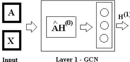
[13] WithV as the node set and E as the dyad set, graph G(V, E) has binary adjacency matrixA∈IR|V|∗|V| and node feature matrixX∈IR|V|∗m. The node feature matrix is formed by horizontally stacking them-dimension feature vector of each node. GCN has the following steps:1. Convolutional filter ˆAis constructed from new adjacency matrix ˜A=A+I and new degree matrix ˜D=D+I by operation ˆA= ˜D−21A˜D˜
−1 2 .
2. A propagation rule for the graph convolution layer is defined as H(1) =
σ( ˆAH(0)θ(0)). H(1) is the matrix of activations of the first layer, H(0) = X,
θ(0) is a trainable weight matrix of layer 0, and σ is a non-linear activation function.
3. The convoluted representations of vertices ˆAH(0) are fed into a standard fully connected layer as shown in Figure 1.
Figure 1. Graph Convolution Neural Network
2.2. Deep learning network representative learning frameworks
Several attempts have been made to overcome the drawbacks of GCN-based archi-tectures for representation learning. Kipfet al.[13] proposed a variant of an existing
GCN-based architecture that uses two layers of feature aggregation so that higher-order dependencies can be captured in the vector embedding of the node. The inputs are adjacency matrix Aand node feature matrixX. In the absence of the node fea-ture matrix, the input can be a matrix with one-hot encoded representations of the nodes. The output of the model is theRd vector embeddings of the nodes of the
in-put graph [13]. One of the negative effects of graph convolutions is that they pushthe encoded representations of neighboring nodes closer to each other [16]. Theoretically, this would mean that the nodes of a graph would converge to a single point in latent space with multiple convolutions.
The framework proposed by M. Defferrard et al. samples a node neighborhood to form sub-graphs using a pooling operation [4]. Feature aggregation is performed on the sub-graphs for generating the final hidden representations of the nodes. The representations are calculated on the sub-graphs instead of on the original graph. This makes the framework more suitable for graph classification than representation learning. The graph auto-encoder with GCN proposed by T. Kipf et al. takes adja-cency matrixAof the entire graph and node feature matrixXas its input. It outputs reconstructed adjacency matrix ˆAand node-embedding matrixZ. The loss function during learning is reconstruction loss, which is calculated asL=Eq(Z|X,A)[logp(A|Z)].
An inner product function is used as decoder ˆA=σ(ZZT). As the encoder function
minimizes the loss due to reconstruction error, the representations of the nodes pre-serve first-order proximity. Global graph features are not considered in such node representations.
The graph spatial-temporal networks with GCN proposed by B. Yuet al.[31] use GCN to learn the representations of the nodes to capture the spatial dependency of the nodes and 1-D CNN to capture the temporal dependency. The framework takes the adjacency matrix at time t and node feature matrix at time t as its input. As temporal information is not available in the case of static graphs, this framework is unsuitable for NRL on static graphs.
The encoder of the graph variational auto-encoder proposed by T. Kipfet al.[14] infers latent variables Z by sampling from a normal distribution. The µ, σ2 of this normal distribution is generated through a two-layer GCN asµ=GCNµ(X, A), σ2=
GCNσ(X, A), GCN(X, A) = AReLUˆ ( ˆAXθ(0))θ(1). Then, for each input xi,
q(Zi|X, A) = N(Zi|µi, diag(σi2)). The decoder uses the same method as the inner
product function of GAEs to obtain reconstructed adjacency matrix A0 =σ(Z.ZT).
The loss function has two parts: first, the construction loss to ensure a reconstructed adjacency matrix is similar to the input one. The second part is KL-divergence to en-sure that the distribution of the latent variable is close to a normal distribution. The graph-VAE model depends on the GCN; hence, the model’s performance is stagnant with multiple stacked layers due to the fully connected layers.
L=Eq(Z|X,A)[logp(X|Z)]−KL(q(Z|X, A)||p(Z)) (1)
where p(Z) =Q
Drawbacks of existing architectures:
•To integrate global graph structural information, a much deeper GCN architec-ture would be required.
•GCN-based architectures cause a dramatic drop in model performance when stacked together [16].
•Excessive parameter due to fully connected layers in encoder.
3. Deep convolutional graph auto-encoder
Figure 2 provides the architecture of the encoder of the GAE with the use of the 1D convolutional (FC) layer in place of the fully connected (dense) layer. These FC encoder blocks are stacked to obtain the encoder of the GAE. The inner product decoder is kept the same.
Figure 2. Architecture of convolutional graph auto-encoder
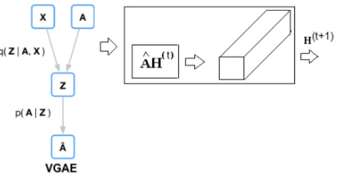
Similar to the 1D convolutional graph auto-encoder, an FC encoder block is used to substitute the fully connected layer in the GVAE as shown in Figure 3.
Figure 3. Architecture of graph variational auto-encoder with fully convolutional layer
3.1. Deep convolutional variational auto-encoders
The two models proposed in Sections 3 and 3.1 are trained to learn the embeddings using the procedure given in Algorithm 1.
The FC auto-encoder architectures are given in Table 1 for the BlogCatalog, CiteSeer, Cora, Flickr, Protein, and Wiki datasets.
Algorithm 1:Model Training and Fitting Data: X, A
Result: Z
1 Initialization of encoder weightsθand biasb; 2 Configure model to minimize Loss in Eq. 2.2;
3 Add activation function: rectified linear unit to encoder; 4 Create inner product decoder layer function;
5 Split data as 75:25 into train and test sets; 6 Set epochs, batch size;
7 Optimize the loss functionLusing gradient descent; Table 1
Description of FC encoder blocks of auto-encoder architectures
Layer name BlogC Cora CiteSeer Flickr Protein Wiki
X 5198*8189 2709*1434 914*3703 7577*12047 3891*50 4778*40
A 5198*5198 2709*2709 914*914 7577*7577 3891*3891 4778*4778
conv encode 1x64 1x64 1x64 1x64 1x4 1x4
stride 1 1 1 1 1 1
padding valid valid valid valid valid valid
conv encode 1x32 1*64 1x64 1x64 1*3 1x3
stride 1 3 2 1 1 1
padding valid valid valid valid valid valid
conv encode 1x32 1*64 1*32 1x32 – –
stride 1 2 2 1 – –
padding valid valid valid valid – –
conv encode 1x32 1x32 1*32 1x32 – –
stride 1 1 1 1 – –
padding valid valid valid valid – –
conv encode 1x32 1*64 – 1x32 – –
stride 1 1 1 1 – –
padding valid valid valid valid – –
conv encode 1*32 1*64 – 1x32 – –
stride 1 2 – 2 – –
padding valid valid – valid – –
conv encode – 1*32 – – – – stride – 2 – – – – padding – valid – – – – conv encode – 1*32 – – – – stride – 1 – – – – padding – valid – – –
-The auto-encoder of the BlogCatalog dataset has six FC encoder blocks, the encoder for the CiteSeer dataset has four FC encoder blocks, the encoder for Cora has eight FC encoder blocks, the encoder of the Flickr dataset has five FC encoder blocks, the encoder for the Protein dataset has two FC encoder blocks, and the encoder for Wiki has two FC encoder blocks.
3.2. Relationship of auto-encoders with laplacian smoothing
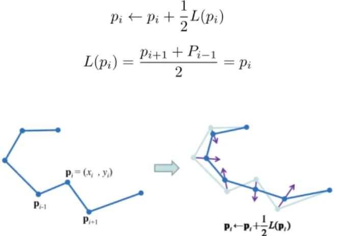
Consider a curve with points pi, pi−1, pi+1. . . as shown in Figure 4. When laplacian smoothing is applied to the graph, it results in each point getting closer to the weighted average of its neighbors as given in Equations (2) and (3).
pi ←pi+ 1 2L(pi) (2) L(pi) = pi+1+Pi−1 2 =pi (3)
Figure 4. Example of laplacian smoothing where curve is shown before and after smoothing operation is applied. Image extracted from [16]
For a graph G= (V, E) with adjacency matrixAsuch that aij = 1,|i−j|= 1,
and degree matrix D=diag(d1, d2, .., dn), the smoothing operation can be rewritten
as Equations (4) and (5): P ←(I−1 2Lrw)P (4) where: P = x1 y1 x2 y2 .. . ... xn yn Lrw= 1 −1 −1 2 1 − 1 2 . .. . .. . .. −1 2 1 − 1 2 −1 1 (5)
Matrix L = D−A is the normalized graph laplacian and has two versions –
Lsym=D−1/2LD−1/2 andLrw=D−1L. The laplacian-smoothing operation isP ←
(I−γLrw)P, and 0≤γ≤1 controls the strength of the smoothing. Settingγ= 0, the
laplacian smoothing becomes equivalent to the non-linear mapping function (identity function) being learned by the auto-encoders. The laplacian smoothing computes the local average of each vertex as its new representation. Since vertices in the same cluster tend to be densely connected, the smoothing makes their features similar, which makes the subsequent representation learning task-amenable.
4. Experiments
All of the datasets are publicly available at [15], and the details of the construction of the features for each data set are mentioned at the source.
4.1. Datasets
CiteSeer – there are 3312 scientific publications as nodes connected by the directed edge to a node if they cite it. There are 4732 links in the network. The feature vector of each node has 3704 features [20].
Cora – this is a citation network of 2708 nodes and 5429 links. The feature vector of each node has 1434 features [11].
BlogCatalog – this is a friendship network of 10,312 and 333,983 links. The feature vector of each node has 8189 features [10].
Flickr-Net – a “follower-following” network of 7575 users with 239,738 links. The feature vector of each node has 12,047 features [10].
Protein-Net – an interaction network of 3890 proteins with 37,845 edge links. The feature vector of each node has 50 features [10].
Wiki-Net – a citation network of Wikipedia articles with 4777 nodes and 54,810 links. The feature vector of each node has 40 features [10].
4.2. Performance metrics
We have used the following performance metrics in the research presented in this paper:
•Separation index: computed based on the distances for each point to the closest point not in the same cluster. The separation index is then the mean. A lower value indicates that the clusters are well separated.
•Widest within-cluster gap: the largest link in a within-cluster minimum span-ning tree is computed. A larger value indicates good clustering.
•Average silhouette width: A measure of how similar an object is to its own cluster as compared to other clusters. The silhouette ranges from −1 to +1, where a high value indicates that the object is well-matched to its own cluster and poorly matched to neighboring clusters.
•Average distance between clusters: for two clustersr, s, the average distance between clusters should be large enough to indicate well-separated clusters as given by Equation (6). L(r, s) = 1 nr∗ns nr X i=1 ns X i=1 D(xri, xsj) (6) •Dunn index: a lower Dunn index indicates better clustering. δ(Ci, Cj) is the
inter-cluster distance metric between clusters Ci and Cj, ∆k is the maximum
within cluster variance as given by Equation (7).
DIm=
min1≤i<j≤mδ(Ci, Cj)
max1≤k≤m∆k
4.3. Results and discussions
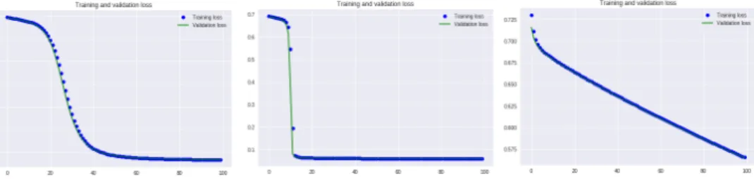
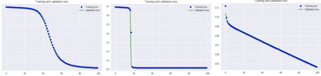
As can be seen in Figure 5, the loss decreases exponentially with the number of epochs in first two models, with a steeper decline in the VAE-FC model. Comparatively, the sparse auto-encoder has a high bias and cannot effectively learn the representations for the data-points in the training set.
Figure 5. Training and cross-validation loss (binary cross-entropy loss) on CiteSeer dataset for graph encoder with fully convolutional layer (GAE-FC), deep variational auto-encoder with fully convolutional layer (VAE-FC), and sparsity constraint auto-auto-encoder [5, 6]
The loss seen in Figure 6 decreases exponentially with the number of epochs in first two models, with a steeper decline in the VAE-FC model. Comparatively, the sparse auto-encoder has a high bias and cannot effectively learn the representations for the data-points in the training set.
Figure 6. Training and cross-validation loss (binary cross-entropy loss) on Cora dataset for graph auto-encoder with fully convolutional layer (GAE-FC), deep variational auto-encoder
with fully convolutional layer (VAE-FC), and sparsity constraint auto-encoder [5, 6]
The application of deep auto-encoders on the graph is equivalent to the appli-cation of multiple laplacian-smoothing operations on the graph. Each hidden layer computes a new latent representation of the data-point that is at a greater proximity to its neighbors. The resultant effect of the operations is that the encoder learns the representations that preserve a Euclidean proximity between the data-points in the latent space.
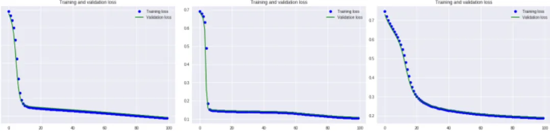
The loss seen in Figure 7 decreases exponentially with the number of epochs in the first two models, with a steeper decline in the VAE-FC model. Comparatively, the
sparse auto-encoder has a high bias and cannot effectively learn the representations for the data-points in the training set. The VAE-FC model computes the represen-tations of the data-points with added constraints of minimizing the Kullback-Leibler divergence between the encoder’s distribution over the representation’s qθ(z|x) and
the distribution of the the latent representations of the data-point’s p(z)∼ N(0,1). This leads to the representation vectors being normally distributed and organized into spherical clusters.
Figure 7. Training and cross-validation loss (binary cross-entropy loss) on BlogCatalog dataset for graph auto-encoder with fully convolutional layer (GAE-FC), deep variational
auto-encoder with fully convolutional layer (VAE-FC), and sparsity constraint auto-encoder [5, 6]
The plot of the training and cross-validation loss vs. the epochs in Figure 8 for a sparsity constraint encoder reveals a high-bias and low-variance model. The sparsity constraints are responsible for the regularization of the model; this further exacerbates the high bias problem. The model fails to effectively capture the representations for the data-points of the network. To reduce the bias, the GAE-FC and VAE-FC models in-troduce additional parameters and more hidden layers. Both of these models are able to generalize to unseen data-points. The loss decreases exponentially with the epochs.
Figure 8. Training and cross-validation loss (binary cross-entropy loss) on Flickr dataset for graph auto-encoders with fully convolutional layer (GAE-FC), deep variational auto-encoder
with fully convolutional layer (VAE-FC), and sparsity constraint auto-encoder [5, 6]
The feature vector of the Protein social network has IR50. The small feature set allows for effective representation learning with sparsity constraint auto-encoders.
The loss with the epochs reduces exponentially for all three models (as can be seen in Fig. 9). The advantage of VAE-FC over the other models is the constraint of minimizing the Kullback-Leibler divergence between the encoder’s distribution over representationsqθ(z|x) and the distribution of the latent representations of the
data-point’s p(z)∼ N(0,1). This leads to the representation vectors being normally dis-tributed and organized into spherical clusters.
Figure 9. Training and cross-validation loss (binary cross-entropy loss) on Protein dataset for graph auto-encoders with fully convolutional layer (GAE-FC), deep variational auto-encoder
with fully convolutional layer (VAE-FC), and sparsity constraint auto-encoder [5, 6]
The feature vector of the Protein social network has IR40. The three models learn representations of the data-points, and the training and cross-validation loss are minimal (as can be seen in Fig. 10). The encoders are able to generalize training parameters over unseen samples in the cross-validation data.
Figure 10. Training and cross-validation loss (binary cross-entropy loss) on Wikipedia dataset for graph auto-encoders with fully convolutional layer (GAE-FC), deep variational
auto-encoder with fully convolutional layer (VAE-FC), and sparsity constraint auto-encoder [5, 6]
Table 2 describes the trainable parameters of the three neural encoder architec-tures. Sparsity constraint encoders have a lower count of parameters and are more suitable for smaller datasets. For larger datasets, the GAE-FC and VAE-FC deep-encoder models would be preferred.
Table 2
Comparison of different neural auto-encoders Description Sparse Enc GAE-FC VAE-FC Parameters 532,317 2,125,469 6,205,263 Training Time per
epoch (in sec) 8 13 25
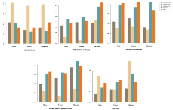
The three encoders were utilized for exploratory data analysis, and the perfor-mance of these models was evaluated on three datasets (see Figs. 11, 12). Hierarchical clustering (AGNES) was used to cluster the representation vectors. Internal cluster validation measures reveal that GAE-FC and VAE-FC obtain better results as com-pared to the simple encoder or sparsity constraint auto-encoders.
Figure 11. Comparison of performance of graph auto-encoders with fully convolutional layer (GAE-FC), deep variational auto-encoder with fully convolutional layer (VAE-FC),
and sparsity constraint auto-encoder [5, 6] on datasets
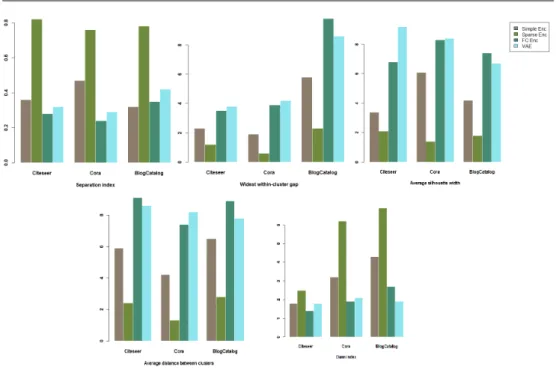
The representations learned by the auto-encoders were clustered using unsu-pervised clustering – AGNES. It was observed that the graph auto-encoders with fully convolutional layers (GAE-FC) and the deep variational auto-encoder with fully convolutional layer (VAE-FC) learned the latent variable model for its input data performed better.
Figure 12. Comparison of performance of graph auto-encoders with fully convolutional layer (GAE-FC), deep variational auto-encoder with fully convolutional layer (VAE-FC),
and sparsity constraint auto-encoder [5, 6] on datasets
5. Conclusion
With the advent of the digital transformation of our society, the generation of data is occurring at an exponential rate. Network models for the representation of data have become popular in scientific domains due to their ease in interpretation as well as analysis. In spite of such considerable advantages in research, networks or graphs are also associated with disadvantages such as the lack of independent observations and the existence of coupling between data-points. Representation learning is pro-posed as a suitable solution for such drawbacks. However, the existing techniques for representation learning are based on heuristics and, hence, cannot capture complex non-linear patterns in the data-points and encode them into representations.
The neural network-based models in the literature focus on semi-supervised learn-ing on graphs. However, as labeled datasets are costly and unavailable in real-world systems, the current investigation was motivated to utilize unsupervised neural archi-tectures such as encoders. It was observed that graph auto-encoders with a fully con-volutional layer (GAE-FC) and a deep variational auto-encoder with a fully convolu-tional layer (VAE-FC) performed significantly better at representation learning when compared to the sparsity constraint architecture. Such architectures were also able to learn representations for data-points not observed in the training phase. This feature
makes them more suitable for deployment on real-world systems than heuristic-based shallow techniques. The operation of aggregation and transformation performed in the hidden layer of a neural network is equivalent to a laplacian-smoothing opera-tion. Hence, deep variational auto-encoders with fully convolutional layer (VAE-FC) architectures learn representations such as data-points associated with similar char-acteristics in the high-dimension space are located in the proximity of the latent space.The experiments performed on the network datasets experimentally validated this theoretical insight.
References
[1] Bandyopadhyay S., Kara H., Kannan A., Murty M.: FSCNMF: Fusing Struc-ture and Content via Non-negative Matrix Factorization for Embedding Infor-mation Networks, arXiv preprint arXiv:1804.05313, 2018. http://arxiv.org/ abs/1804.05313.
[2] Barab´asi A.L.: Network science. Cambridge University Press, 2016.
[3] Cui P., Wang X., Pei J., Zhu W.: A Survey on Network Embedding, IEEE Transactions on Knowledge and Data Engineering, vol. 31(5), pp. 833–852, 2019.
https://doi.org/10.1109/TKDE.2018.2849727.
[4] Defferrard M., Bresson X., Vandergheynst P.: Convolutional Neural Networks on Graphs With Fast Localized Spectral Filtering. In: NIPS’16: Proceedings of the 30th International Conference on Neural Information Processing Systems, pp. 3844–3852, 2016.
[5] Deng J., Zhang Z., Marchi E., Schuller B.: Sparse Autoencoder-Based Feature Transfer Learning for Speech Emotion Recognition. In: 2013 Humaine Associa-tion Conference on Affective Computing and Intelligent InteracAssocia-tion, pp. 511–516, IEEE, 2013.
[6] Deng L., Seltzer M.L., Yu D., Acero A., Mohamed A., Hinton G.: Binary Cod-ing of Speech Spectrograms UsCod-ing a Deep Auto-Encoder. In: Eleventh Annual Conference of the International Speech Communication Association, 2010. [7] Denny M.: Social network analysis, Institute for Social Science Research,
Uni-versity of Massachusetts, Amherst, 2014.
[8] Denny M.: Intermediate Social Network Theory, Institute for Social Science Re-search, University of Massachusetts, Amherst, 2015.
[9] Goyal P., Ferrara E.: Graph Embedding Techniques, Applications, and Perfor-mance: A Survey,Knowledge Based Systems, vol. 151, pp. 78–94, 2018.
[10] Hamilton W.L., Ying R., Leskovec J.: Inductive Representation Learning on Large Graphs. In: Proceedings of the 31st Conference on Neural Information Processing Systems (NIPS 2017), pp. 1024–1034, 2017.
[11] Hamilton W.L., Ying R., Leskovec J.: Representation Learning on Graphs: Meth-ods and Applications,arXiv preprint arXiv:1709.05584, 2017.
[12] Jackson M.O.: Social and Economic Networks, Princeton University Press, 2010. [13] Kipf T.N., Welling M.: Semi-Supervised Classification with Graph Convolutional
Networks,arXiv preprint arXiv:1609.02907, 2016.
[14] Kipf T.N., Welling M.: Variational Graph Auto-Encoders, arXiv preprint arXiv:1611.07308, 2016.
[15] Leskovec J., Krevl A.: SNAP Datasets: Stanford Large Network Dataset Collec-tion, 2014.http://snap.stanford.edu/data.
[16] Li Q., Han Z., Wu X.M.: Deeper Insights Into Graph Convolutional Networks for Semi-Supervised Learning. In: Thirty-Second AAAI Conference on Artificial Intelligence, 2018.
[17] Mikolov T., Chen K., Corrado G., Dean J.: Efficient Estimation of Word Repre-sentations in Vector Space,arXiv preprint arXiv:1301.3781, 2013.
[18] Nerurkar P., Chandane M., Bhirud S.: A Comparative Analysis of Community Detection Algorithms on Social Networks. In: Computational Intelligence: The-ories, Applications and Future Directions, vol. I, pp. 287–298, Springer, 2019. [19] Nerurkar P., Shirke A., Chandane M., Bhirud S.: A Novel Heuristic for
Evolu-tionary Clustering,Procedia Computer Science, vol. 125, pp. 780–789, 2018. [20] Nikolentzos G., Meladianos P., Tixier A.J.P., Skianis K., Vazirgiannis M.: Kernel
Graph Convolutional Neural Networks. In: International Conference on Artificial Neural Networks, pp. 22–32, Springer, 2018.
[21] Ou M., Cui P., Pei J., Zhang Z., Zhu W.: Asymmetric Transitivity Preserving Graph Embedding. In:Proceedings of the 22nd ACM SIGKDD International Con-ference on Knowledge Discovery and Data Mining, pp. 1105–1114, ACM, 2016. [22] Pandhre S., Mittal H., Gupta M., Balasubramanian V.N.: STwalk: learning tra-jectory representations in temporal graphs. In: CoDS-COMAD ’18: Proceedings of the ACM India Joint International Conference on Data Science and Manage-ment of Data, pp. 210–219, ACM, 2018.
[23] Rozemberczki B., Davies R., Sarkar R., Sutton C.: GEMSEC: Graph Embedding with Self Clustering,arXiv preprint arXiv:1802.03997, 2018.
[24] Rozemberczki B., Sarkar R.: Fast Sequence Based Embedding with Diffusion Graphs. In: International Conference on Complex Networks, 2018.
[25] Tran P.V.: Learning to Make Predictions on Graphs with Autoencoders, arXiv preprint arXiv:1802.08352, 2018.
[26] Tsitsulin A., Mottin D., Karras P., M¨uller E.: VERSE: Versatile Graph Embed-dings from Similarity Measures. In: Proceedings of the 2018 World Wide Web Conference on World Wide Web, pp. 539–548, International World Wide Web Conferences Steering Committee, 2018.
[27] Veliˇckovi´c P., Cucurull G., Casanova A., Romero A., Li`o P., Bengio Y.: Graph Attention Networks,arXiv preprint arXiv:1710.10903, 2017.
[28] Wang Z., Ye X., Wang C., Wu Y., Wang C., Liang K.: RSDNE: Exploring Re-laxed Similarity and Dissimilarity from Completely-imbalanced Labels for Net-work Embedding. In: The Thirty-Second AAAI Conference on Artificial Intelli-gence (AAAI-18), pp. 475–482, 2018.
[29] Wu Z., Pan S., Chen F., Long G., Zhang C., Yu P.S.: A Comprehensive Survey on Graph Neural Networks,arXiv preprint arXiv:1901.00596, 2019.
[30] Yang Z., Cohen W.W., Salakhutdinov R.: Revisiting Semi-Supervised Learning With Graph Embeddings,arXiv preprint arXiv:1603.08861, 2016.
[31] Yu B., Yin H., Zhu Z.: Spatio-Temporal Graph Convolutional Networks: A Deep Learning Framework for Traffic Forecasting. In: Proceedings of the International Joint Conference on Artificial Intelligence, pp. 3634–3640, 2018.
[32] Zhang M., Cui Z., Neumann M., Chen Y.: An End-to-End Deep Learning Archi-tecture for Graph Classification. In: Proceedings of AAAI Conference on Artificial Inteligence, pp. 4438–4445, 2018.
[33] Zhou J., Cui G., Zhang Z., Yang C., Liu Z., Wang L., Li C., Sun M.: Graph Neural Networks: A Review of Methods and Applications, arXiv preprint arXiv:1812.08434, 2018.
Affiliations
Pranav Ajeet Nerurkar
VJTI, Computer Engineering and IT Department, Mumbai, India, ORCID ID: https://orcid.org/0000-0002-9100-6437
Madhav Chandane
ORCID ID: https://orcid.org/0000-0002-2872-4647
Sunil Bhirud
ORCID ID: https://orcid.org/0000-0002-9100-6437
Received: 24.01.2019 Revised: 30.05.2019 Accepted: 30.05.2019