Ensembles of Random Sphere Cover Classifiers
Reda Younsi and Anthony Bagnall
aUniversity of East Anglia, Norwich Research Park, UK bUniversity of East Anglia, Norwich Research Park, UK
Abstract
We propose and evaluate a new set of ensemble methods for the Randomised Sphere Cover (RSC) classifier. RSC is a classifier using the sphere cover method that bases classification on distance to spheres rather than distance to instances. The randomised nature of RSC makes it ideal for use in ensembles. We propose two ensemble methods tailored to the RSC classifier;αβRSE, an ensemble based on instance resampling andαRSSE, a subspace ensemble. We compareαβRSE andαRSSE to tree based ensembles on a set of UCI datasets and demonstrates that RSC ensembles perform significantly better than some of these ensembles, and not significantly worse than the others. We demonstrate via a case study on six gene expression data sets that αRSSE can outperform other subspace ensemble methods on high dimensional data when used in conjunction with an attribute filter. Finally, we perform a set of Bias/Variance decomposition experiments to analyse the source of improvement in comparison to a base classifier.
Keywords: Sphere Cover, Ensemble, B/V decomposition
1. Introduction
Combining the predictions of a set of randomised classifiers has been very successful in classification [16]. Bagging and Boosting are two popular com-bination methods using randomised sampling methods [54]. That is, they are
∗Corresponding author
used to combine predictions of various classifiers by randomly selecting training subsets. However, a large family of instance based classifiers (IB) are unable to use randomisation. We introduce novel algorithms that combines several IB classifiers based on sphere covers, where each member of the ensemble builds random data-dependent sphere covers.
The proposed ensemble methods use the Randomised Sphere Cover (RSC) classifier, first introduced in [53]. RSC creates spheres around a subset of in-stances from the training data, then bases classification on distance to spheres, rather than distance to instances. RSC is similar to Nearest neighbour (NN) based classifiers which are very popular in machine learning for their simplicity and highly efficient data compression [53]. One of their strength as stand-alone classifiers lies in the fact that they are robust to changes in the training data. However, this feature of NN classifiers means that there is less observable benefit (in terms of error reduction) of using them in conjunction with known ensemble schemes such as bagging [3] and boosting [14]. RSC aims to overcome this prob-lem by using a randomised heuristic to select a subset of instances to represent the spheres used in classification. RSC is powerful data reduction algorithm as shown in [53]. Data reduction algorithms [51, 27, 24] search the training data for a subset of cases and/or attributes with which to classify new instances to achieve the maximum compression with the minimum reduction in accuracy.
The sphere cover classifier can be described by the Compression scheme first described in Floyd [13]. The Compression scheme has been proposed to explain the generalisation performance of sparse algorithms. In general, algorithms are called sparse because they retain a small subset from the training set as part of their learning process. For example, a Support Vector Machine (SVM) with a small number of support vectors or a condensed NN classifier could be consid-ered sparse. Recently, compression scheme was rejuvenated to explore a similar algorithm to the sphere cover, called set covering machine (SCM), proposed by Marchand and Shawe-Taylor [43]. The process that creates the spheres for sphere cover is controlled by two parameters: α, the minimum number of cases a sphere must contain in order to be retained as part of the classifier; and β,
the number of misclassified instances a sphere can contain. Younsi [54], ex-amined the relationships between α, the accuracy and the cardinality of the sphere cover classifier using existing probabilistic bound based on the compres-sion scheme. Although it is clear the sphere cover accuracy is synonymous with covering, compression scheme experiments have shown that degradation is ac-curacy is only possible by heavily pruning spheres [54]. This suggests that the randomised sphere cover classifier is indeed a strong candidate for exploring the accuracy/diversity dilemma found in ensemble design [25, 41, 46, 28].
We propose two ensemble methods tailored to the RSC classifier;αβRSE, an ensemble based on resampling andαRSSE, a subspace ensemble. We investigate howαand β parameters can be optimally used to diversify the ensemble. We demonstrate that the resulting ensemble classifiers are comparable to, and often better than, state of the art ensemble techniques. We perform a case study on six high dimensional gene expression data sets to demonstrate thatαRSSE works well with attribute filters and that it outperforms other subspace ensemble methods on these data sets. Finally, we perform a set of Bias/Variance (BV) decomposition experiments to analyse the source of improvement in comparison to a base classifier.
The structure of the rest of this paper is as follows: In Section 2 we provide the background motivation for the RSC classifier, an overview of the relevant ensemble literature and a brief summary of Domingos BV decomposition tech-nique [10]. In Section 3 we formally describe the RSC classifier and in Section 4 we define our two ensemble schemes. In Section 5 we present the results and in Section 7 we summarise our conclusions.
2. Background
A classifier constructs a decision rule based on a set of l training examples
D={(xi, yi)}li=1, wherexirepresents a vector of observations ofmexplanatory variables associated with the ith case, and y
i indicates the class to which the
ithexample belongs. We call the range of all possible values of the explanatory variablesXand the range of the discrete response variableY={C1, C2, . . . , Cr}.
We assume a dissimilarity measuredis defined onXand is a functiond:X×X→ R+ such that ∀x1,x2 ∈ X, d(x1,x1) = 0 and d(x1,x2) = d(x2,x1) ≥ 0. A
classifier f : X → Y, f(x) = ˆy is a function from the attribute space to the response variable space.
2.1. Sphere Cover Classifiers
The sphere covering mechanism we use stems from the class covering ap-proach to classification which was first introduced in [6]. A sphereBi is asso-ciated with a particular classCBi, and is defined by a centre ci and radiusri. In practice we also include in the sphere definition all the instances within it’s boundary. Hence, a sphere is defined by a 4-tuple
Bi=< CBi,ci, ri, XBi >
where XBi = {x ∈ D : d(x,ci)< ri}. The centre of the sphere is the vector of the means of the attributes of the cases contained within. The radius of the sphereBi is defined as the distance from the centre to the closest example from a class other thanCBi that is not in XBi, i.e.
ri= min
xj∈{X\XBi}∧yj̸=CBi
d(xj,ci)
where X = {x ∈ D}. A union of spheres is called a cover. A cover that contains all of the examples inDis calledproperand one consisting of spheres that only contain examples of one class is said to be pure. The class cover problem (CCP) involves finding a pure and proper cover that has the minimum number of spheres of all possible pure and proper covers.
The solution to the CCP proposed in [38] involves constructing a Class Cover Catch Digraph (CCCD), a directed graph based on the proximity of training cases. However, finding the optimal covering via the CCCD is NP-hard [7]. Hence [33, 32] proposed a number of greedy algorithms to find an approximately optimal set covering. However, these algorithms are still slow and only find pure covers.
The constraint of pure and proper covers will tend to lead to a classifier that overfits the training data. An algorithm that relaxes the requirement of class
purity was proposed by [38]. This algorithm introduces two parameters to alle-viate the constraint of requiring a pure proper cover. The parameterαrelaxes the proper requirement by only allowing spheres that contain at leastα cases to be retained in the classifier. The parameterβ reduces the purity constraint by allowing a sphere to contain β cases of the wrong class. The authors ad-mit the resulting algorithms are infeasible for large data and hence (to the best of our knowledge) there has been very limited experimental evaluation of this and other CCP based classifiers. Furthermore, the resulting classifiers are very sensitive to the parameters. In particular, β, if constant for all spheres, is too crude a mechanism for relaxing the purity constraint. In Section 3 we describe an ensemble base classifier derived from CCP algorithm proposed in [34] that is randomised (rather than constructive) and retains just the single parameter,α.
2.2. Ensemble Methods
An ensemble of classifiers is a set of base classifiers whose individual decisions are combined through some process of fusion to classify new examples [35, 9]. One key concept in ensemble design is the requirement to inject diversity into the ensemble [9, 42, 37, 16, 17, 19]. Broadly speaking, diversity can be achieved in an ensemble by either:
• employing different classification algorithms to train each base classifier to form a heterogeneous ensemble;
• changing the training data for each base classifier through a sampling scheme or by directed weighting of instances;
• selecting different attributes to train each classifier;
• modifying each classifier internally, either through re-weighting the train-ing data or through inherent randomization.
Clearly, these approaches can be combined (see below). In this paper we com-pare our homogeneous ensemble methods (described in Section 4) with the fol-lowing related ensembles.
• Bagging[3] diversifies through sampling the training data by bootstrap-ping (sampling with replacement) for each member of the ensemble.
• Random Subspace[21] ensembles select a random subset of attributes for each base classifier.
• AdaBoost (Adaptive Boosting) [14] involves iteratively re-weighting the sampling distribution over the training data based on the training accuracy of the base classifiers at each iteration. The weights can then be either embedded into the classifier algorithm or used as a weighting in a cost function for classifier selection for inclusion.
• Random Committeeis a technique that creates diversity through ran-domising the base classifiers, which in Weka are a form of random tree.
• Multiboost [49] is a combination of a boosting strategy (similar to Ad-aBoost) and wagging, a Poisson weighted form of bagging.
• Random Forests[4] combine bootstrap sampling with random attribute selection to construct a collection of unpruned trees. At each test node the optimal split is derived by searching a random subset of size K of candidate attributes selected without replacement from the candidate attributes. Random forest random combines attribute sampling with bootstrap case sampling.
• Rotation Forests[41] involve partitioning the attribute space then trans-forming in to the principal components space. Each classifier is given the entire data set but trains on a different component space.
In order to maintain consistency across these techniques we use C4.5 decision trees [39] as the base classifier for all the ensembles.
Forming a final classification from an ensemble requires some sort of fu-sion. We employ a majority vote fusion [29] with ties resolved randomly. For alternative fusion schemes see [26].
Beyond simple accuracy comparison, there are three common approaches to analyse ensemble performance: diversity measures [30, 46]; margin theory [40, 35]; and BV decomposition [23, 47, 15, 5, 48, 2]. These have all been linked [46, 10].
2.3. Bias/Variance Decomposition
In this section, we briefly describe BV decomposition using Domingos frame-work [10]. This frameframe-work is applicable to any loss function, but for simplicity sake we restrict ourselves to a two class classification problem with a 0/1 loss function. We label the two class values{C1=−1, C2= 1}. The generalisation
error of a classifier is defined as the expected error for a given loss function over the entire attribute space. A loss functionL(y,yˆ) measures how close the predicted value is from the actual value for any observation (x, y). The response variableY will generally be stochastic, so for a two class problem the expected loss is defined as
Ey[L(y,yˆ)] =p(Y =−1|x)·L(0,yˆ) +p(Y = 1|x)·L(1,yˆ),
and the optimal predictiony∗is the prediction that mimimizes the expected loss. The optimal or Bayes classifier is one that minimizes the expected loss for all possible values of the attribute space, i.e. f(x) =y∗,∀x∈X. The expected loss over the attribute space of the Bayes classifier,
Ex[Ey[L(y, y∗)]]
, more commonly writtenEx,y[L(y, y∗)] is called the Bayes rate and is the lower
bound for the error of any classifier.
In practice, classifiers are constructed with a finite data set, and the expected loss for any given instance will vary depending on which data set the classifier is given.
LetDbe a set ofstraining sets,D={{Di}si=1}. The set of predictions for
any elementxis then ˆY ={yˆi, i= 1· · ·s}, where ˆyi is the prediction of theith classifier defined on training dataDi when given explanatory variables x. We
then denote the mode of ˆY as the main prediction, ˆy. If we assume each data set is equally likely to have been observed, the expected loss oversdata sets for a given instancexis simply the average over the data sets,
ED,y[L(y,yˆ)] =
∑s
i=1Ey[L(y,yˆi)] s
The Domingos framework decomposes this expected loss into three terms: Bias, Variance and Noise. The Bias is defined as the loss of the main prediction in relation to the optimal prediction.
B(x) =L(y∗,yˆ)
Bias is caused by systemic errors in classification resulting from the algorithm not capturing the underlying complexity of the true decision boundary (i.e. un-derfitting). Variance describes the mean variation within the set of predictions about the main prediction for a given instance, i.e.,
V(x) =
∑s
i=1L( ˆyj,yˆ)
s ,
and is the result of variability of the classification function caused by the finite training sample size and the hence inevitable variation across training samples (overfitting). Noise is the unavoidable (and unmeasurable) component of the loss that is incurred independently of the learning algorithm. The Noise term is
N(x) =E[L(y, y∗)].
So for a single example, we can describe the expected loss as
ED,y[L(y,yˆ)] =N(x) +B(x) +c2·V(x)
wherec2 is +1 ifB(x) = 0 and−1 ifB(x) = 1.
Bias and variance may be averaged over all examples, in which case Domin-gos calls them average Bias, B = Ex[B(x)], average (or net variance) V = Ex[V(x)] and average noiseN =Ex(N(x)). The expected loss over all
exam-ples is the expected value of the expected loss over all examexam-ples, and can be decomposed as
ED,y,x[L(y,yˆ)] =N+B+c2·V
.
Domingos shows that the net variance can be expressed as
V =Ex[(2B(x)−1)·V(x)]
and thatV can be further deconstructed into thebiased varianceVb and the unbiased varianceVu. Vu is the average variance within the set of classifier estimates where the main prediction is correct (B(x) = 0), Vb is the variance when the main prediction is incorrect. The net variance Vn is the difference between the unbiased and the biased variance,Vn =Vu−Vb. Hence, unbiased variance increases the net variance (and thus the generalisation error) whereas biased variance decreases the net variance.
The principle benefit of performing a Bias-Variance (BV) decomposition for an ensemble algorithm is to address the question of whether an observed reduction in the expected loss is due to a reduction in bias, a reduction in unbiased variance, an increase in biased variance or, more usually, a combination of these factors. Without unlimited data, these statistics are generally estimated through resampling. In Section 6 we describe our experimental design and perform a BV decomposition to assess the ensemble algorithms we propose in Section 4 in conjunction with the base classifier described in Section 3.
3. The Randomised Sphere Cover Classifier (RSC)
The reason for designing the αRSC algorithm was to develop an instance based classifier to use in ensembles. Hence our design criteria were that it should be randomised (to allow for diversity), fast (to mitigate against the inevitable overhead of ensembles) and comprehensible (to help produce meaningful inter-pretations from the models produced). TheαRSCalgorithm has a single integer parameter,α, that specifies the minimum size for any sphere. Informally,αRSC
• Repeat until all data are covered or discarded
1. Randomly select a data point and add it to the set of covered cases. 2. Create a new sphere centered at this point.
3. Find the closest case in the training set of a different class to the one selected as a centre.
4. Set the radius of the sphere to be the distance to this case. 5. Find all cases in the training set within the radius of this sphere. 6. If the number of cases in the sphere is greater thanα, add all cases
in the sphere to the set of covered cases and save the sphere details (centre, class and radius).
A more formal algorithmic description is given in Algorithm 1. For all our experiments we use the Euclidean distance metric, although the algorithm can work with any distance function. All attributes are normalised onto the range [0,1]. The parameter α allows us to smooth the decision boundary, which Algorithm 1 buildRSC(D,d,α). A Randomised Sphere Cover Classifier (αRSC)
1: Input: Cases D = {(x1, y1), . . . ,(xn, yn)}, distance function d(xi,xj)
pa-rameterα.
2: Output: Set of spheresB 3: Let covered cases be setC=⊘
4: Let uncovered cases be setU =⊘
5: whileD̸=C∪U do
6: Select a random element (xi, yi)∈D\C 7: Copy (xi, yi) toC
8: Find min(xj,yj)∈Dd(xi,xj) such thatyi̸=yj
9: Letri=d(xi,xj)
10: Create aBi with a centerci=xi, radiusri and target classyi
11: Find all the cases inBi and store in temporary setT
12: if |T| ≥αthen 13: C=C∪T
14: Store the sphereBi inB
15: else
16: U =U∪T 17: end if
has been shown to provide better generalisation by mitigating against noise and outliers, (see, for example [31]). Figure 1 provides an example of the smoothing effect of removing small spheres on the decision boundary.
(a) A sphere cover withα= 1 (b) The same cover withα= 2
Figure 1: An example of the smoothing effect of removing small spheres
TheαRSC algorithm classifies a new case by the following rules:
1. Rule 1. A test example that is covered by a sphere, takes the target class of the sphere. If there is more than one sphere of different target class covering the test example, the classifier takes the target class of the sphere with the closest centre.
2. Rule 2. In the case where a test example is not covered by a sphere, the classifier selects the closest spherical edge.
This approach is similar to the classification rule from the CCCD, which scales the distances to the sphere centres by the radii and picks the smallest.
A case covered by Rule 2 will generally be an outlier or at the boundary of the class distribution. Therefore, it may be preferable not to have spheres over-covering areas where such cases may occur. These areas are either close to the decision boundary specifically when the high overlap between classes exist (an illustration is given in Figure 1 (a)), and areas where noisy cases are
within dense areas of examples of different target class. The αRSC method of compressing through sphere covering and smoothing via boundary setting as first proposed in [53] and has been shown to provides a robust simple classifier that is competitive with other commonly used classifiers [53]. In this paper we focus on the best way to use it as a base classifier for an ensemble.
4. Ensemble Methods forαRSC
4.1. A Simple Ensemble: αRSE
One of the basic design criteria forαRSC was to randomise the cover mecha-nism so that we could create diversity in an ensemble. Hence our first ensemble algorithm, αRSE, is simply a majority voting ensemble of αRSC classifiers. With all ensembles we denote the number of classifiers in the ensemble as L. We fixα for all members of the ensemble. Each classifier is built using Algo-rithm 1 using the entire training data. The basic question we experimentally assess is whether the inherent randomness of αRSC provides enough implicit diversity to make the ensemble robust.
4.2. A Resampling/Re-weighting Ensemble: αβ RSE
The original motivation for RSC is the classifiers derived from the Class Cover Catch Digraph (CCCD) described in Section 2. These classifiers have two parameters, αand β. The αparameter (minimum sphere size) is used to improve generalisation. Theβ parameter (number of misclassified examples al-lowed within a sphere) is meant to filter outliers. In the CCCD, bothαandβ
parameters are chosen in advance. αcan be set through cross validation. How-ever, settingβ is problematic; a global value ofβ is too arbitrary, a local value for each sphere impractical. We propose an automatic method for implicitly settingβ iteratively.
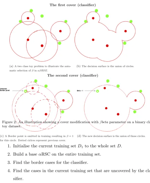
We define theborder case of a sphere to be the closest data with a class label different to that of the sphere. Border cases are the particular instance that halts the growth of a sphere and are hence crucial in the construction of theαRSC classifier. Our design principle for diversification of the ensemble is
then to iteratively remove some or all of the border cases during the process of ensemble construction. Informally, the algorithm proceeds as follows:
Figure 2: An illustration showing a cover modification with/betaparameter on a binary class toy dataset.
1. Initialise the current training setD1 to the whole setD.
2. Build a baseαRSC on the entire training set. 3. Find the border cases for the classifier.
4. Find the cases in the current training set that are uncovered by the clas-sifier.
5. Find the cases in the entire training set that are misclassified by the clas-sifier.
6. Set the next training set,D2, equal toD1.
7. Remove border cases fromD2.
8. Replace the border cases with a random sample (with replacement) taken from the list of border, uncovered and misclassified cases and add them toD2.
9. Repeat the process for each of theL classifiers.
Algorithm 2A Randomised Sphere Cover Ensemble (αβ RSE)
Input: Cases D={(x1, y1), . . . ,(xn, yn)}, distance functiond(xi,xj),
parame-tersα, L.
Output: L random sphere cover classifiersB1, . . . , BL
1: D1=D 2: forj= 1 toLdo 3: Bj =buildRSC(Dj,d, α). 4: E=borderCases(Bj, Dj) 5: F =uncoveredCases(Bj, Dj) 6: G=misclassifiedCases(Bj, D) 7: H =E+F+G 8: Dj+1=Dj−E 9: form= 1 to|E|do 10: c=randomSample(H) 11: Dj+1=Dj+1 ∪ c 12: end for 13: end for
A formal description is given in Algorithm 2. New cases are classified by a majority vote of the L classifiers. The principle idea is that we re-weight the training data by removing border cases, thus facilitating spheres that are not pure on the original data, but continue to focus on the harder cases by inserting possible duplicates of border, uncovered or misclassified cases, thus implicitly re-weighting the training data. Data previously removed from the training data can be replaced if misclassified on the current iteration. This data driven iterative approach has strong analogies to constructive algorithms such as boosting.
4.3. A Random Subspace Ensemble: αRSSE
As outlined in Section 2.2, rather than resampling and/or re-weighting for ensemble members, an alternative approach to diversification is to present each base classifier with a different set of attributes with which to train. The Random Subspace Sphere Cover Ensemble (αRSSE) builds base classifiers using random subsets of attributes by sampling without replacement from the original full attribute set. Each base classifier has the same number of attributes, κ. The attributes used by a classifier are also stored, and the same set of attributes are used to classify a test example. The majority vote is again employed for the final hypothesis.
Algorithm 3A Random Subspace Sphere Cover Ensemble (αRSSE) Input: Cases D={(x1, y1), . . . ,(xn, yn)},d(xi,xj), parameters α,L,κ. Output: Lrandom sphere cover classifiersB1, . . . , BLand associated attribute setsK1, . . . , KL. 1: forj= 1 toLdo 2: Kj=randomAttributes(D, κ) 3: Dj =filterAttributes(D, Kj) 4: Bj =buildRSC(Dj,d, α) 5: end for 5. Accuracy Comparisons
Our base classifierαRSC is a competitive classifier in its own right, achieving accuracy results comparable to C4.5, Naive Bayes, Naive Bayes Tree, K-Nearest Neighbour and the Non-Nested Generalised Hyper Rectangle classifiers [50]. We wish to compare the performance ofαRSC based ensembles with equivalent tree based ensemble techniques. Our experimental aims are:
1. To confirm that ensembling αRSC improves the performance of the base classifier (Section 5.2).
2. To show that the RSC ensembleαβRSE performs better than tree based ensembles that utilise the whole feature space (Section 5.3).
3. To demonstrate that the RSC ensembleαRSSE performs significantly bet-ter than all the subspace ensembles except rotation forest, which itself is not significantly better thanαRSSE (Section 5.4).
4. To consider, through a cases study, whetherαRSC ensembles outperform other subspace ensemble methods on classification problems with a high dimensional feature space (Section 5.5).
To assess the relative performance of the classifiers, we adopt the procedure described in [8], which is based on a two stage rank sum test. The first test, the Freidman F test is a non-parameteric equivalent to ANOVA and tests the null hypothesis that the average rank ofk classifiers onndata sets is the same against the alternative that at least one classifier’s mean rank is different. If the Friedman test results in a rejection of the null hypothesis (i.e. we reject the hypothesis that all the mean ranks are the same), Demˇsar recommends a post-hocpairwise Nemenyi test to discover where the differences lie. The performance of two classifiers is significantly different if the corresponding average ranks differ by at least the critical difference
CD=qa
√
k(k+ 1) 6n ,
wherekis the number of classifiers,nthe number of problems andqais based on the studentised range statistic. The results of apost-hocNemenyi test are shown in the critical difference diagrams (as introduced in [8]). These graphs show the mean rank order of each algorithm on a linear scale, with bars indicatingcliques, within which there is no significant difference in rank (see Figure 4 below for an example). Alternatively, if one of the classifiers can be considered a control, it is more powerful to test for difference of mean rank between classifier iand j
based on a Bonferonni adjustment. Under the null hypothesis of no difference in mean rank between classifieriandj, the statistic
z=√(¯ri−¯rj) k(k+1)
6n
follows a standard normal distribution. If we are performing (k−1) pairwise comparisons with our control classifier, a Bonferonni adjustment simply divides
the critical valueαby the number of comparisons performed.
5.1. Data Sets
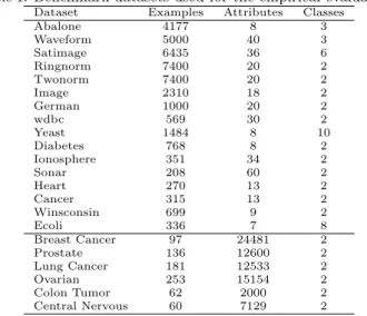
Table 1:Benchmark datasets used for the empirical evaluations
Dataset Examples Attributes Classes
Abalone 4177 8 3 Waveform 5000 40 3 Satimage 6435 36 6 Ringnorm 7400 20 2 Twonorm 7400 20 2 Image 2310 18 2 German 1000 20 2 wdbc 569 30 2 Yeast 1484 8 10 Diabetes 768 8 2 Ionosphere 351 34 2 Sonar 208 60 2 Heart 270 13 2 Cancer 315 13 2 Winsconsin 699 9 2 Ecoli 336 7 8 Breast Cancer 97 24481 2 Prostate 136 12600 2 Lung Cancer 181 12533 2 Ovarian 253 15154 2 Colon Tumor 62 2000 2 Central Nervous 60 7129 2
To evaluate the performance of the ensembles we used sixteen datasets from both the UCI data repository [11] and six benchmark gene expression datasets from [44]. These datasets are summarised in Table 1. They were selected be-cause they vary in the numbers of training examples, classes and attributes and thus provide a diverse testbed. In addition, they all have only continuous at-tributes, and this allows us to fix the distance measure for all experiments to Euclidean distance. All the features are normalised onto a [0,1] scale. The first sixteen data are used for all classification experiments in Sections 5.3 and 5.4. The six gene expression data sets are used for experiments presented in Sec-tion 5.5 to evaluate how the subspace based ensembles perform in conjuncSec-tion with a feature selection filter on a problem with high dimensional feature space.
5.2. Base Classifier vs Ensemble
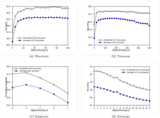
As a basic sanity check, we start by showing that the ensemble outperforms the base classifier by comparing αβRSE with 25 base classifiers against the average of 25αRSC classifiers. Figure 3 shows the graphs of the classification
accuracy (measured through 10 fold cross validation) for four different datasets. The ensemble accuracies are better than those of the 25 averaged classifiers, and this pattern was consistent across all data sets. In addition, we notice both curves follow a similar evolution in relation toα. That is, α values that returned the best classification accuracy forαβ RSE are similar to those of a single classifier. This is the motivation for the model selection method we adopt in Section 5.3. Alpha (Prunng #) 0 20 40 60 80 100 Accuracy 85.0 86.0 87.0 88.0 89.0 90.0 91.0 Ensemble 10 CV accuracy Average 10 CV accuracy (a)Waveform Alpha (Pruning #) 0 100 200 300 400 500 Accuracy 93.0 94.0 95.0 96.0 97.0 98.0 Ensemble 10 CV accuracy Average 10 CV accuracy (b)Twonorm Alpha (Pruning #) 0 1 2 3 4 % training examples 93.0 94.0 95.0 96.0 97.0 98.0 Ensemble 10CV accuracy Average qocv accuracy
(c)Ringnorm Alpha (Pruning #) 0 1 2 3 4 5 6 7 8 9 10 11 12 13 14 15 16 17 Accuracy 84 86 88 90 92 94 Ensemble 10 CV accuracy Average 10 CV accuaracy (d)Satimage
Figure 3: Accuracy as a function ofα on four data sets. Each point is the ten fold
cross validation accuracy ofαβRSE with 25 classifiers and the average of 25 separate
αRSC classifiers
5.3. Full Feature Space Ensembles
Tables 2 and 3 show the classification accuracy ofαRSE andαβRSE against that of Adaboost, Bagging and Multiboost trained with 25 and 100 base
classi-fiers respectively. Adaboost, Bagging and Multiboost were used with the default settings for the decision tree and ensemble parameters and were trained on the full training split.
For αRSE and αβRSE,αwas set through a quick form of model selection by using the optimal training set cross validation values of a single classifier. This form of quick, off-line model selection is possible because of the fact that RSC is controlled by just a single parameter and has little impact on the overall time taken to build the ensemble classifier. As described in Section 4.2, theβ
parameter ofαβRSE is set implicitly through the sampling scheme.
The average ranks and rank order are given in the final two rows of Table Tables 2 and 3. The critical difference for a test of difference in average rank for 5 classifiers and 16 data sets at the 10% level is 1.375.
Table 2:mean classification accuracy (in %) and standard deviation ofαβRSE,αRSE, Adaboost, Bagging, and Multiboost over 30 different runs on independent train/test splits with 25 base classifiers.
Data Set αRSE αβRSE Adaboost Bagging MultiBoost Abalone 54.25±0.94 54.89±1.02 52.30±1.20 53.98±0.91 53.04±1.47 Waveform 90.40±0.67 90.68±0.65 89.60±0.69 88.71±0.58 89.63±0.56 Satimage 90.90±0.41 90.90±0.41 91.21±0.45 89.82±0.69 90.94±0.57 Ringnorm 96.71±0.38 97.17±0.30 97.26±0.33 95.01±0.50 97.12±0.31 Twonorm 97.32±0.26 97.41±0.26 96.43±0.32 95.58±0.46 96.41±0.37 Image 96.87±0.50 96.87±0.51 97.77±0.64 95.78±0.90 97.32±0.75 German 73.21±1.76 74.00±1.69 74.52±1.76 75.24±1.36 75.09±2.51 wdbc 93.21±1.47 93.86±1.52 96.79±1.26 95.19±1.38 96.61±1.22 Yeast 56.34±2.09 58.22±1.24 58.23±1.59 60.65±1.57 58.65±1.77 Diabetes 74.52±1.78 75.01±1.79 73.54±1.88 75.94±2.00 74.74±2.34 Iono 93.48±2.05 93.39±2.25 92.85±2.20 92.31±2.60 93.25±2.05 Sonar 84.67±4.17 84.43±3.66 81.38±4.21 76.33±5.66 80.76±4.57 Heart 78.85±3.60 80.74±3.26 80.41±3.11 81.26±3.66 81.22±2.87 Cancer 69.46±2.97 70.07±3.62 69.07±4.36 73.44±2.87 69.35±4.71 Winsc 95.53±1.34 95.67±1.33 96.21±0.84 96.01±0.97 96.49±0.71 Ecoli 85.36±2.78 85.51±2.64 83.07±2.75 83.45±3.58 83.45±2.73 Average Ranks 3.31 2.50 3.13 3.28 2.78 Ranking 5 1 3 4 2
We make the following observations from these results:
• Firstly, although αβRSE has the highest rank, we cannot reject the null hypothesis of no significant difference between the mean ranks of the clas-sifiers. The performance of the simple majority vote ensemble αRSE is comparable to bagging with decision trees. This suggests that the base classifier αRSC inherently diversifies as much as bootstrapping decision
Table 3:mean classification accuracy (in %) and standard deviation ofαβRSE,αRSE, Adaboost, Bagging, and Multiboost over 30 different runs on independent train/test splits with 100 base classifiers.
Data Set αRSE αβRSE Adaboost Bagging MultiBoost Abalone 54.36±1.16 54.48±1.23 52.82±0.99 54.1±0.91 54.22±1.47 Waveform 90.56±0.70 90.32±0.66 90.27±0.58 89.08±0.84 90.20±0.93 Satimage 90.91±0.38 91.12±0.44 92.00±0.39 90.47±0.55 91.11±0.60 Ringnorm 96.88±0.37 97.54±0.31 97.75±0.29 95.23±0.52 97.05±0.52 Twonorm 97.36±0.28 97.49±0.22 97.13±0.26 96.35±0.38 96.95±0.27 Image 96.77±0.50 96.80±0.56 97.98±0.56 96.23±0.80 96.71±0.34 German 73.23±1.82 74.16±1.58 74.46±1.54 74.91±1.85 74.70±0.64 wdbc 93.39±1.56 93.91±1.57 96.91±1.55 96.33±1.35 96.47±1.07 Yeast 57.26±1.44 58.41±1.36 58.13±1.62 60.08±1.56 59.57±1.22 Diabetes 74.53±1.84 75.04±2.57 73.53±2.20 75.68±2.57 74.54±1.28 Iono 93.56±2.06 93.53±1.96 92.99±2.29 91.20±3.01 92.39±2.25 Sonar 84.86±4.23 85.00±3.72 82.71±5.14 78.57±5.86 82.71±2.21 Heart 79.26±3.40 80.67±3.10 81.19±2.88 81.56±3.59 82.33±4.20 Cancer 69.53±3.29 69.58±3.32 68.82±5.07 73.19±3.34 71.33±3.51 Winsc 95.54±1.33 95.71±1.33 96.48±0.88 96.09±0.94 97.00±4.31 Ecoli 85.54±2.96 85.86±2.65 83.07±2.75 83.45±3.58 84.82±0.75 Average Ranks 3.38 2.38 3.03 3.44 2.78 Ranking 4 1 3 5 2
trees and lends support to usingαRSC as a base classifier.
• Secondly, αβRSE outperforms αRSE on 12 out of 16 data sets (with 2 ties) with 25 bases classifiers and 14 out of 16 with 100 base classifiers. If we were performing a single comparison between these two classifiers, the difference would be significant. Whilst the multiple classifier comparisons mean we cannot make this claim, the results do indicate that allowing some misclassification and guiding the sphere creation process through directed resampling does improve performance and that a simple ensemble does not best utilise the base classifier.
• Thirdly,αβRSE has the highest average rank of the five algorithms, from which we infer that it performs at least comparably to Adaboost, Multi-boost and performs better than Bagging. These experiments demonstrate that the re-weighting based ensembleαβRSE is at least comparable to the widely used tree based sampling and/or re-weighting ensembles.
5.4. Subspace Ensemble Methods
Tables 4 and 5 show the classification accuracy of αRSSE against those of Rotation Forest, Random Subspace, Random Committee and Random Forest ensembles of decision trees, based on 25 and 100 classifiers.
Table 4:Classification accuracy (in %) and standard deviation ofαRSSE, Rotation For-est (RotF), Random SubSpace (RandS), Random ForFor-est (RandF) and Random Com-mittee (RandC) using average results of 30 different runs on independent train/test splits with 25 base classifiers.
Data Set αRSSE RotF RandS RandF RandC
Abalone 54.77±1.28 55.56±1.04 54.62±1.09 54.05±1.16 53.56±1.19 Waveform 90.21±0.51 90.72±0.77 89.35±0.73 89.51±0.61 89.32±0.61 Satimage 91.71±0.47 91.03±0.50 90.79±0.54 90.80±0.52 90.24±0.44 Ringnorm 98.29±0.26 97.57±0.23 96.82±0.35 95.49±0.38 96.6±0.30 Twonorm 97.03±0.30 97.42±0.27 95.88±0.33 96.02±0.37 96.18±0.35 Image 97.39±0.65 98.04±0.51 96.42±0.73 97.27±0.63 96.08±0.58 German 74.59±1.47 76.26±1.63 72.28±1.53 74.85±1.46 73.65±1.77 wdbc 94.67±1.33 96.40±1.03 95.35±1.31 95.30±1.42 96.04±1.26 Yeast 58.80±1.90 61.06±1.82 57.38±2.45 58.96±1.69 60.26±1.75 Diabetes 76.17±2.25 76.25±2.30 74.48±1.98 75.43±1.92 74.78±1.51 Iono 94.53±1.79 93.50±1.79 92.68±2.40 93.05±1.86 93.13±2.33 Sonar 84.52±4.49 82.86±4.50 79.57±5.24 81±4.68 82.19±3.99 Heart 82.74±4.02 82.74±3.32 83.30±3.55 81.67±3.17 81.00±3.62 Cancer 76.27±2.96 73.87±3.29 74.73±2.81 71.18±3.74 70.93±4.29 Winsc 97.21±0.95 97.18±0.83 96.35±1.01 96.48±0.72 97.00±0.84 Ecoli 85.00±2.07 87.41±2.44 84.02±3.13 85.33±2.76 84.82±2.62 Mean Ranks 2.09 1.53 4.00 3.50 3.88 Ranks 2 1 5 3 4
Table 5: Classification accuracy (in %) and standard deviation of αRSSE, Rotation Forest (RotF), Random SubSpace (RandS), Random Forest (RandF) and Random Committee RandC) using average results of 30 different runs on independent train/test splits with 100 base classifiers.
Data Set αRSSE RotF RandS RandF RandC
Abalone 54.91±0.98 56.04±1.04 54.79±1.02 54.47±0.86 52.83±0.95 Waveform 90.73±0.53 91.07±0.77 89.68±0.62 89.97±0.62 90.36±0.63 Satimage 91.92±0.54 91.70±0.50 91.28±0.55 91.59±0.46 91.82±0.46 Ringnorm 98.43±0.27 97.77±0.23 97.22±0.35 95.66±0.43 97.70±0.26 Twonorm 97.39±0.28 97.53±0.27 96.24±0.51 96.38±0.50 97.22±0.27 Image 97.83±0.53 98.16±0.51 96.78±0.62 97.45±0.62 97.93±0.56 German 74.28±1.56 75.69±1.63 72.37±1.06 75.63±0.64 74.79±1.86 wdbc 95.00±1.44 96.75±1.03 96.35±1.49 96.95±1.17 97.11±1.32 Yeast 59.43±1.93 61.65±1.82 58.94±1.84 60.03±1.31 58.22±1.57 Diabetes 76.25±2.21 76.12±2.30 74.84±2.07 75.14±2.04 74.00±2.02 Iono 94.76±1.68 94.19±1.79 92.74±1.80 92.39±1.77 93.33±1.94 Sonar 85.24±5.39 84.43±4.50 79.62±5.62 82.05±4.44 82.24±4.63 Heart 84.00±3.43 83.30±3.15 83.41±3.92 82.70±3.35 81.22±4.50 Cancer 76.16±2.75 74.12±3.29 75.30±2.85 71.36±4.41 68.82±5.07 Winsc 97.42±0.91 97.38±0.83 96.60±0.98 96.71±0.90 96.47±0.78 Ecoli 85.71±2.36 87.41±2.44 84.02±3.13 85.33±2.76 83.45±2.73 Mean Ranks 1.94 1.69 4.06 3.50 3.81 Ranks 2 1 5 3 4
As with αβRSE, the αRSSE parameters α and κ were set through cross validation on one third of the training set. The optimal value ofκwas estimated first, then the best value ofαfound for thatκ. The other ensembles were trained on the entire training set with default parameters.
Figure 4 shows the Critical Difference diagram for the subspace methods with 25 base classifiers. There is a significant difference in average rank
be-tween the classifiers (the F statistic is 14.97, which gives a P value of less than 0.00001). This difference can be described by two clear cliques: Random Sub-space, Random Committee and Random Forest are significantly outperformed by the cliqueαRSSE and Rotation Forest. The fact thatαRSSE out performs Random Forest is particularly impressive in light of recent evidence that it is highly competitive over a wide range of data [12]. Rotation Forest beatsαRSSE on nine data sets, loses on 6 and ties on one. A pairwise comparison ofαRSSE and Rotation Forest using the Wilcoxon signed rank test, a paired t-test and a binomial test indicates no significant difference between Rotation Forest and
αRSSE. The p-values are 0.366, 0.24 and 0.301 respectively.
CD 5 4 3 2 1 1.5313 RotFor 2.0938 aRSSE 3.5 RandFor 3.875 RandComm 4 RandSub
Figure 4: Critical difference diagram for 5 subspace ensembles on 16 data sets. Critical difference is 1.375.
So whilst rotation forest has a lower average rank thanαRSSE on these data sets, the difference is not significant.
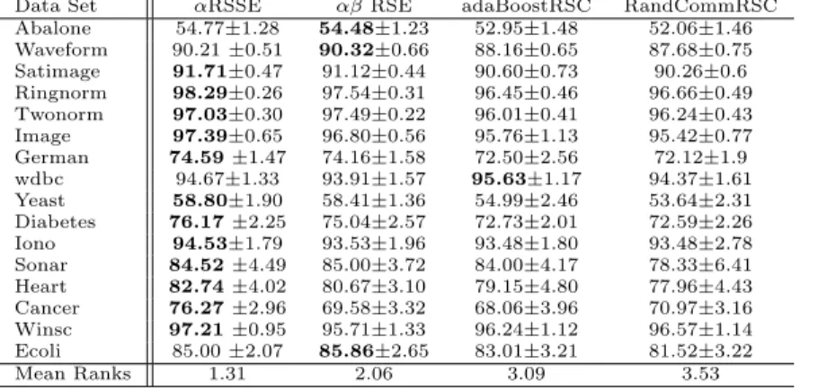
Ensemble schemes such as adaBoost are designed to improve the performance of weak learner classifiers. However, there is nothing in principle to stop one using RSC as a base classifier for one of these schemes. Table 6 compares our results for αRSSE and αβ RSE with adaBoost and random committee using RSC as a base classifier. αRSSE is significantly better than the RSC versions of adaBoost and random committee.
Table 6: Classification accuracy (in %) and standard deviation of αRSSE, αβ RSE adaBoost with RSC as a base classifier and Random Committee usingRSC as a base classifier. Results are averaged over 30 different runs on independent train/test splits with 25 base classifiers. The critical difference is 1.17.
Data Set αRSSE αβRSE adaBoostRSC RandCommRSC Abalone 54.77±1.28 54.48±1.23 52.95±1.48 52.06±1.46 Waveform 90.21±0.51 90.32±0.66 88.16±0.65 87.68±0.75 Satimage 91.71±0.47 91.12±0.44 90.60±0.73 90.26±0.6 Ringnorm 98.29±0.26 97.54±0.31 96.45±0.46 96.66±0.49 Twonorm 97.03±0.30 97.49±0.22 96.01±0.41 96.24±0.43 Image 97.39±0.65 96.80±0.56 95.76±1.13 95.42±0.77 German 74.59±1.47 74.16±1.58 72.50±2.56 72.12±1.9 wdbc 94.67±1.33 93.91±1.57 95.63±1.17 94.37±1.61 Yeast 58.80±1.90 58.41±1.36 54.99±2.46 53.64±2.31 Diabetes 76.17±2.25 75.04±2.57 72.73±2.01 72.59±2.26 Iono 94.53±1.79 93.53±1.96 93.48±1.80 93.48±2.78 Sonar 84.52±4.49 85.00±3.72 84.00±4.17 78.33±6.41 Heart 82.74±4.02 80.67±3.10 79.15±4.80 77.96±4.43 Cancer 76.27±2.96 69.58±3.32 68.06±3.96 70.97±3.16 Winsc 97.21±0.95 95.71±1.33 96.24±1.12 96.57±1.14 Ecoli 85.00±2.07 85.86±2.65 83.01±3.21 81.52±3.22 Mean Ranks 1.31 2.06 3.09 3.53
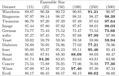
We further note that the difference in performance between rotation forest and αRSSE reduces with an increase in the number of base classifiers. Table 7 shows the classification accuracy (calculated through 10CV) of αRSSE for various sizes of ensemble, varying from 15 to 500 base classifiers. In general, ensembles perform better when the size of the ensemble is large. However, with many ensemble methods increasing the ensemble size dramatically results in over training and hence lower testing accuracy. Table 7 demonstrates that the performance of αRSSE actually improves with over 100 base classifiers, indicating αRSSE does not have a tendency to over fit data sets with large ensemble sizes.
Figure 5 shows the combined critical difference diagram for all 10 ensembles. The increase in the number of ensembles means a much larger critical difference is required to detect a significant difference. However, a similar pattern of ranking is apparent.
Theno free lunch theorem[52] convinces us there will not be a single dom-inant algorithm for all classification problems. Instance based approaches are still popular in a range of problem domains, particularly in research areas re-lating to image processing and databases. αβRSE and αRSSE offer instance
Table 7: αRSSE 10CV accuracy for ensemble sizes of 15 to 500. Ensemble Size Dataset (15) (25) (50) (100) (250) (500) Waveform 89.87 90.38 90.72 90.85 91.21 90.97 Ringnorm 97.97 98.14 98.27 98.31 98.37 98.39 Twonorm 96.79 97.20 97.39 97.49 97.63 97.64 Image 97.44 97.80 97.92 97.87 98.01 98.03 German 74.77 75.43 75.52 75.47 75.52 75.66 wdbc 97.27 97.45 97.75 97.68 97.99 97.98 Yeast 59.02 59.79 59.56 59.58 59.86 59.94 Diabetes 76.89 76.95 76.96 77.03 77.21 76.96 Iono 95.09 95.37 95.23 95.11 95.46 95.43 Sonar 86.85 87.81 88.30 88.69 88.03 88.47 Heart 81.74 84.26 83.85 83.63 83.81 83.96 Cancer 75.54 75.88 76.05 77.06 76.93 77.30 Winsc 97.08 97.34 97.24 97.40 97.38 97.33 Ecoli 86.17 86.45 86.57 86.15 86.62 86.60 CD 10 9 8 7 6 5 4 3 2 1 2.0625 RotFor 2.6875 aRSSE 7.0625 alphaRSE 7.4063 Bagging
Figure 5: Critical difference diagram for 10 ensembles on 16 data sets. Critical difference is 3.1257.
based approaches to classification problems that are highly competitive with the best tree based subspace and non-subspace ensemble techniques. In the following Section we propose a type of problem domain where we thinkαRSSE outperforms the tree based ensembles.
5.5. Gene Expression Classification Case Study: Subspace Ensemble Compari-son
Gene expression profiling helps to identify a set of genes that are responsible for cancerous tissue. In the last decade, microarray gene expression cancer diagnosis showed promising results using various classification algorithm. In this section we test the performance ofαRSSE algorithm on six gene expression datasets. We choose to use three feature reduction methods that are popular in bioinformatics [45]. In addition, biologists seek the smallest set possible of genes to reduce laboratory experimentation cost. Thus, removing redundancy early on in the process helps reduce the classification running cost in relation to the size of genes (features).
5.5.1. Gene Expression Datasets
This section gives a brief description of gene expression datasets used in our empirical evaluation.
1. Breast Cancer
This dataset is made of patients outcome prediction for breast cancer. The original file is made of a training and testing datasets. The training data con-tains 78 patient samples, 34 of which are from patients who had developed distance metastases within 5 years (labelled as relapse), the rest 44 samples are from patients who remained healthy from the disease after their initial diagnosis for interval of at least 5 years (labelled as non-relapse). Correspondingly, there are 12 relapse and 7 non-relapse samples in the testing data set. The number of genes is 24481.
2. Central Nervous System
Patients outcome prediction for central nervous system embryonal tumor. Survivors are patients who are alive after treatment whiles the failures are those who succumbed to their disease. The data set contains 60 patient samples, 21 are survivors (labelled as ‘Class1’) and 39 are failures (labelled as ‘Class0’). There are 7129 genes in the dataset.
3. Colon Tumor
The Colon dataset Contains 62 samples collected from colon cancer patients. Among them, 40 tumor biopsies are from tumors (labelled as ‘positive’) and 22 normal (labelled as ‘Negative’) biopsies are from healthy parts of the colons of the same patients. Two thousand out of around 6500 genes were selected based on the confidence in the measured expression levels.
4. Lung Cancer (Dana-Farber Cancer Institute, Harvard Medical School)
A total of 203 snap-frozen lung tumors and normal lung were analysized. The 203 speciments include 139 samples of lung adenocarcinomas (labelled as ADEN), 21 samples of squamous cell lung carcinomas (labelled as SQUA), 20 samples of pulmonary carcinoids (labelled as COID), 6 samples of small-cell lung carcinomas (labelled as SCLC) and 17 normal lung samples (labelled as NORMAL). Each sample is described by 12600 genes.
5. Ovarian Cancer (NCI PBSII Data)
The proteomic spectra were generated by mass spectroscopy and the data set provided here is 6-19-02, which includes 91 controls (Normal) and 162 ovarian cancers. The raw spectral data of each sample contains the relative amplitude of the intensity at each molecular mass / charge (M/Z) identity. There are
total 15154 M/Z identities. The intensity values were normalized according to the formula: NV = (V-Min)/(Max-Min), where NV is the normalized value, V the raw value, Min the minimum intensity and Max the maximum intensity. The normalization is done over all the 253 samples for all 15154 M/Z identities. After the normalization, each intensity value is to fall within the range of 0 to 1.
6. Prostate Cancer
Tumor versus Normal classification: training set contains 52 prostate tumor samples (labelled as ‘Positive’) and 50 non-tumor (labelled as ‘Normal’) prostate samples with around 12600 genes. The dataset was given as a training set and test set. We simply concatenated the training and testing files then use random train/test splits in the experiments.
Table 8: The best test set accuracy (in %) ofαRSSE (αR), Rotation Forest (RotF), Random Subspace (RandS), Random Forest (RandF), Adaboost (AB), Bagging (Bag)
and MultiBoostAB (Multi) using average results of 30 different runs onχ2. BC=Breast
Cancer, CT=Colon Tumor, LC=Lung Cancer, OV=Ovarian and PR=Prostrate
Dataset αR RotF RandS RandF AB Bag Multi BC 82.93 79.60 76.26 80.91 79.19 78.99 78.79 CN 77.83 76.83 74.33 80.33 76.33 76.17 76.50 CT 85.87 86.19 83.49 84.13 82.38 83.65 82.86 LC 99.34 99.34 95.03 99.34 97.81 97.21 97.87 OV 99.18 99.80 97.88 98.98 97.73 97.84 97.73 PR 94.13 93.70 91.30 94.57 91.23 91.38 91.09 F-avg 1.75 2.10 5.83 1.92 5.58 5 5.58 F-ranks 1 3 7 2 5.5 4 5.5
Table 9: The best test set accuracy (in %) using average results of 30 different runs on Information Gain.
Dataset αR RotF RandS RandF AB Bag Multi BC 85.15 79.39 77.47 83.94 79.49 80.10 79.80 CN 79.17 76.50 73.50 80.00 75.67 76.17 76.00 CT 86.98 84.76 82.54 84.44 82.70 82.54 82.38 LC 99.34 99.34 94.75 99.34 97.76 97.16 97.81 OV 99.25 99.76 98.00 98.86 97.73 97.88 97.73 PR 93.77 93.48 91.74 93.62 91.09 92.32 90.80 F-avg 1.42 2.75 5.92 2.08 5.42 4.58 5.58 F-ranks 1 3 7 2 5 4 6
Table 10: The best test set accuracy (in %) using average results of 30 different runs on Relief.
Dataset αR RotF RandS RandF AB Bag Multi BC 80.20 79.19 72.42 78.18 73.74 74.85 73.23 CN 76.00 75.50 72.17 76.00 74.00 72.00 73.33 CT 83.65 84.76 80.63 83.33 79.37 83.17 79.68 LC 99.34 99.23 94.75 98.91 97.43 96.61 97.49 OV 98.43 99.37 98.04 98.90 97.61 97.69 97.61 PR 89.13 93.33 91.67 93.62 93.41 89.71 93.26 F-avg 2.58 2.00 5.67 2.25 4.92 5.33 5.25 F-ranks 3 1 7 2 4 6 5
Table 11:The best test set accuracy (in %) using the three attribute ranking methods.
Dataset αR RotF RandS RandF Adaboost Bagging Multi BC 84.04 79.60 77.47 83.94 79.49 80.10 79.80 CN 79.17 76.83 74.33 80.33 76.33 76.17 76.5 CT 86.98 86.19 83.49 84.44 82.70 83.65 82.86 LC 99.34 99.34 95.03 99.34 97.81 97.21 97.87 OV 99.18 99.76 98.00 98.98 97.73 97.88 97.73 PR 94.13 93.70 91.74 94.57 93.41 92.32 93.26 F-avg 1.58 2.58 6.17 1.92 5.58 5.00 4.92 F-ranks 1 3 7 2 6 5 4
large number of attributes [18]: employ a filter that uses a scoring method to rank the attributes independently of the classifier; use a wrapper to score subsets of attributes using the classifier to produce the model; or embed the attribute selection as part of the algorithm to build the classifier [36]. We focus on three simple, commonly used, filter measures, χ2, Information Gain (IG)
and Relief, which are used to select a fixed number of attributes by ranking each on how well they split the training data, in terms of the response variable. We compare αRSSE to Adaboost, Bagging, Random Committee, Multiboost, Random Subspaces, Random Forest and Rotation Forest. Our methodology is to filter on k = 5, 10, 20 30, 40 and 50 best ranked attributes for the three ranking measures. Model selection for αRSSE is conducted as described in Section 5.3. All the ensembles use 100 classifiers. For Adaboost, Bagging and the base decision tree classifiers in the ensembles we use the default parameters. Tables 8, 9 and 10 show the relative performance of the eight ensemble classifiers on the best attribute filter setting for each of the filter techniques. We note that
αRSSE is ranked highest overall when using χ2 and Information Gain and is
filteringαRSSE can overcome the inherent problem instance based learners have with high dimensional attribute spaces to produce results better than the state of the art tree based ensembles classifiers.
6. Bias Variance Analysis of RSC Ensemble Techniques
The purpose of our bias/variance analysis of the ensembles αβRSE and
αRSSE is to identify whether the reduction in generalisation error in compar-ison to the base classifier is due to a reduction in bias, unbiased variance or an increase in biased variance. We followed a similar experimental framework found in [48]. The standard experimental design for BV decomposition is to es-timate Bias and Variance using small training sets and large test sets. We used bootstrapping to sample eight of our datasets. Initially, one third of the data is removed to constitute the test set. 200 separate training bootstrap samples of size 200 were taken by uniformly sampling with replacement from the remaining data. The boostrap training sample is on average less than half the size of the test data. We then compute the main prediction, bias and both the unbiased and biased variance, and net-variance (as defined in Section 2.3) over the 200 test sets.
Figure 6 showing both bias and variance in relation to κ (number of at-tributes used in each classifier forαRSSE) for four of the datasets. We observe there is a strong relationship between averaged error and bias for smallκ, but that as κincreases variance contributes a larger component to the error. In-creasing κ seems to have a higher influence on unbiased variance reduction than biased variance. To compare αRSC, αβRSE and αRSSE, we perform the bias/variance experiment on the three classifiers with the optimal set of parameters (determined experimentally).
We conclude from the above results that αβRSE, in most cases, reduces the net variance in comparison with a single classifier because of a decrease in unbiased variance. However, it is not straight forward in relation to bias. It might be that bias reduction depends on the geometrical complexity of the
sample [22] (complex structures require complex decision boundaries), the cho-sen values for the pruning parameterα, and the interaction betweenαand β. In that case, finding a method that systematically reduces bias while keeping unbiased variance low will further reduce the ensemble average error.
Table 12 shows the bias/variance decomposition of αRSSE, αβRSE and
αRSC. We make the following observations from these results:
1. The average error ofαRSSE and αβRSE is lower thanαRSC for all the problems;
2. ForαβRSE, this is more commonly a result of a reduction in net variance rather than a reduction in bias;
3. ForαRSSE, whilst bias is reduced, we also see a more consistent reduction in variance.
These experiments reinforce our preconception as to the effectiveness of the ensembles: αβRSE introduces further diversity into the ensemble through al-lowing misclassified instances within the spheres. The major effect of this is to reduce the variance of the resulting classifier. On the other hand, the subspace ensemble reduces the inherent bias commonly observed in instance based classi-fiers used in conjunction with a Euclidean distance metric: redundant attributes result in overfitting.
7. Conclusion
We have described an instance based classifier,αRSC, that has several inter-esting properties that can be used successfully in ensemble design. We described three different ensemble methods with which it could be used and demonstrated that the resulting ensembles are competitive with the best tree based ensemble techniques on a wide range of standard datasets. We further investigated the reasons for the improvement in performance of the ensembles in relation to the base classifier using bia/variance decomposition. For the ensemble based on resampling (αβRSE) accuracy was increased primarily by a reduction in vari-ance. Hence we conclude the diversity introduced via the proposed technique is
mostly beneficial and the resulting ensemble classifier is more robust. We also demonstrated through bia/variance decomposition that the subspace ensemble
αRSSE improves performance primarily by a decrease in bias. An obvious next step would be to embed the resampling technique within the random subspace ensemble. However, we found employing theβ mechanism in the subspace did not make a significant difference to the αRSSE ensemble. This implies that attribute selection is the most important stage in ensemblingαRSC, other than model selection by settingα. This has lead us into investigating embedding at-tribute selection (rather than randomisation) into the ensemble, with promising preliminary results. We believe thatαRSC is a useful edition to the family of instance based learners since it is easy to understand, quick to train and test and can effectively be employed in ensembles to achieve classification accuracy comparable to the most popular ensemble methods.
[1] D. Aha, D. Kibler and M.K. Albert: Instance-based learning algorithms, Machine Learning, vol. 6, no. 1, pp.37-66, 1991.
[2] E. Bauer and R. Kohavi: An empirical comparison of voting classification algorithms: bagging, boosting, and variants, Machine Learning, vol. 36, no. 1-2, pp. 105-139, 1999.
[3] L. Breiman: Bagging predictors, Machine Learning, vol. 24, no. 2, pp. 123-140, 1996.
[4] L. Breiman: Random forests, Machine Learning, vol. 45, no. 1, pp. 5-32, 2001.
[5] L. Breiman: Bias, variance, and arcing classifiers, Statistics Department, Berkeley, technical report, no. 460, 1996.
[6] A. Cannon and L.J. Cowen: Approximation algorithms for the class cover problem, Annals of Mathematics and Artificial Intelligence, vol. 40,no. 3-4, pp. 215-223, 2004.
[7] A. Cannon, J. Mark Ettinger, D. Hush, C. Scovel: Machine learning with data dependent hypothesis classes, The Journal of Machine Learning Re-search, vol. 2, pp. 335-358, 2002.
[8] J. Demˇsar: Statistical comparisons of classifiers over multiple data sets. Journal of Machine Learning Research, vol. 7, pp. 1-30, 2006.
[9] T.G. Dietterich: An experimental comparison of three methods for con-structing ensembles of decision trees: bagging, boosting, and randomiza-tion, Machine Learning, vol. 40, no. 2, pp. 139-157, 2000.
[10] P. Domingos: A unified bias-variance decomposition for zero-one and squared loss, Proceedings of the Seventeenth National Conference on Ar-tificial Intelligence and Twelfth Conference on Innovative Applications of Artificial Intelligence, pp. 564-569, 2000.
[11] M. Lichman: UCI Machine Learning Repository, University of California, Irvine, School of Information and Computer Sciences, http://archive.ics.uci.edu/ml, 2013.
[12] M. Fern´andez-Delgado, E. Cernadas, S. Barro and D. Amorim: Do we Need Hundreds of Classifiers to Solve Real World Classification Problems? Journal of Machine Learning Research , vol 15. pp. 3133-3181, 2014 [13] S. Floyd and M. Warmuth: Sample compression, learnability, and the
vapnik-chervonenkis dimension. Machine Learning, vol 21, no. 5. pp. 269-304, 1995
[14] Y. Freund and R.E. Schapire: Experiments with a new boosting algorithm, ICML, pp. 148-156, 1996.
[15] J.H. Friedman and U. Fayyad: On bias, variance, 0/1-loss, and the curse-of-dimensionality, Data Mining and Knowledge Discovery, vol. 1, pp. 55-77, 1997.
[16] P. Geurts and D. Ernst and L. Wehenkel: Extremely randomised trees, Machine Learning, vol. 63, no. 1, pp. 3-42, 2006.
[17] Y. Grandvalet, S. Canu and S. Boucheron: Noise injection: theoretical prospects, Neural Computation, vol. 9, no. 5, pp. 1093-1108, 1997.
[18] I. Guyon and A. Elisseeff: An introduction to variable and feature selection, Journal of Machine Learning Research, vol. 3, pp. 1157-1182, 2003. [19] L.K. Hansen and P. Salamo: Neural network ensembles, IEEE Transactions
on Pattern Analysis and Machine Intelligence, vol. 12, no. 10, pp. 993-1001, 1990.
[20] R. Herbrich: Learning Kernel Classifiers, Theory and Algorithms. MIT Press Cambridge, MA, USA, 2002.
[21] T.K. Ho: The random subspace method for constructing decision forests, IEEE Transactions on Pattern Analysis and Machine Intelligence, vol. 20, no. 8, pp. 832-844, 1998.
[22] T.K. Ho: Geometrical complexity of classification problems, Proceedings of the 7th Course on Ensemble Methods for Learning Machines at the International School on Neural Nets, 2004.
[23] G. James: Variance and bias for general loss functions, Machine Learning, vol. 51, pp. 115-135, 2003.
[24] S.W. Kim and B.J. Oommen: A brief taxonomy and ranking of creative prototype reduction schemes, Pattern Anal. Appl., vol. 6, no. 3, pp. 232-244, 2003.
[25] L.I. Kuncheva: That Elusive Diversity in Classifier Ensembles, Lecture Notes in Computer Science, pp. 1126-1138, 2003.
[26] L.I. Kuncheva: A theoretical study on six classifier fusion strategies, Jour-nal: IEEE Transactions on Pattern Analysis and Machine Intelligence, vol. 24, no. 2, pp. 281-286, 2002.
[27] L.I. Kuncheva and J.C. Bezdek: Presupervised and postsupervised proto-type classifier design, IEEE Transactions on Neural Networks, vol. 10, no. 5, pp. 1142-1152, 1999.
[28] L.I. Kuncheva and C.J. Whitaker, Measures of Diversity in Classifier En-sembles and Their Relationship with the Ensemble Accuracy, Machine Learning, vol .51, pp. 181-207, 2003.
[29] L.I. Kuncheva, C. Whitaker, C. Shipp and R.P.W Duin: Limits on the ma-jority vote accuracy in classifier fusion, Pattern Analysis and Applications, vol. 6, no. 1, pp. 22-31, 2003.
[30] L.I. Kuncheva: Diversity in multiple classifier systems, Information Fusion, vol. 6, no. 1, pp. 3-4, 2005.
[31] H. Liu and H. Motoda: On issues of instance selection, Data Mining and Knowledge Discovery, vol. 6, no. 2, pp. 115-130, 2002.
[32] D.J. Marchette: Random graphs for statistical pattern recognition, Wiley-Interscience, 2004.
[33] D.J. Marchette and C.E. Priebe: Characterizing the scale dimension of a high-dimensional classification problem. Pattern Recognition, vol. 36, no. 1, pp. 45-60, 2003.
[34] D.J. Marchette D., E.J. Wegman and C.E. Priebe: A fast algorithm for approximating the dominating set of a class cover catch digraph, technical report, JHU DMS TR 635, 2003.
[35] R. Meir and G. R¨atsch: An introduction to boosting and leveraging, Ma-chine Learning Summer School, Springer, pp. 118-183, 2002.
[36] L.C. Molina, L. Belanche and A. Nebot: Feature selection algorithms: a survey and experimental evaluation, IEEE International Conference on Data Mining, pp. 306-313, 2002.
[37] D. Opitz and R. Maclin, Popular ensemble methods: an empirical study, Journal of Artificial Intelligence Research, vol. 11, pp. 169-198, 1999. [38] C.E. Priebe, J.G. DeVinney, D.J. Marchette and D.A. Socolinsky:
Classi-fication using class cover catch digraphs. Journal of ClassiClassi-fication, vol. 20, no. 1, pp. 003-023, 2003.
[39] J. R. Quinlan: C4.5: Programs for Machine Learning. Morgan Kaufmann, 1993.
[40] G. Raetsch and T. Onoda and K.R. Mueller: Soft margins for adaboost, Machine Learning, vol. 42, no. 3, 287-320, 2001.
[41] J.J. Rodriguez and L.I. Kuncheva and C.J. Alonso: Rotation forest: a new classifier ensemble method, IEEE transactions on pattern analysis and machine intelligence, vol. 28, no. 10, pp. 1619-1630, 2006.
[42] R.E Schapire: Theoretical views of boosting and applications, International Workshop on Algorithmic Learning Theory, pp. 13-25, 1999.
[43] M. Marchand and J. Shawe-Taylor: The Set Covering Machine, Journal of Machine Learning Research, vol.3, pp. 723-746, 2002.
[44] G. Stiglic and P. Kokol. GEMLeR: Gene Expression Machine Learning Repository. Available at: http://gemler.fzv.uni-mb.si/.
[45] Y. Saeys, I. Inza and P. Larraaga: A review of feature selection techniques in bioinformatics. Bioinformatics, 2007, vol. 23, no. 19.
[46] E.K. Tang, P.N. Suganthan and X. Yao: An analysis of diversity measures, Machine Learning, vol. 65, no. 1, pp. 247-271, 2006.
[47] R. Tibshirani: Bias, variance and prediction error for classification rules, University of Toronto, Dept. of Statistics, Toronto, 1996.
[48] G. Valentini and T.G. Dietterich: Bias-variance analysis of support vector machines for the development of SVM-based ensemble methods, Journal of Machine Learning Research, vol. 5, pp. 725-775, 2004.