"Time Series Nonparametric Regression Using Asymmetric Kernels with an Application to Estimation of Scalar Diffusion Processes"

CIRJE Discussion Papers can be downloaded without charge from: http://www.e.u-tokyo.ac.jp/cirje/research/03research02dp.html

Discussion Papers are a series of manuscripts in their draft form. They are not intended for circulation or distribution except as indicated by the author. For that reason Discussion Papers may not be reproduced or distributed without the written consent of the author.

CIRJE-F-573

Time Series Nonparametric Regression Using

Asymmetric Kernels with an Application to

Estimation of Scalar Diffusion Processes

Nikolay Gospodinov

Concordia University and CIREQ

Masayuki Hirukawa

Northern Illinois University

June 2008

Time Series Nonparametric Regression Using

Asymmetric Kernels with an Application to

Estimation of Scalar Diffusion Processes

Nikolay Gospodinov

_{Masayuki Hirukawa}

Concordia University and CIREQ

Northern Illinois University

December 2007

Abstract

This paper considers a nonstandard kernel regression for strongly mixing processes when the regressor is nonnegative. The nonparametric regression is implemented using asymmetric kernels [Gamma (Chen, 2000b), Inverse Gaussian and Reciprocal Inverse Gaussian (Scaillet, 2004) kernels] that possess some appealing properties such as lack of boundary bias and adaptability in the amount of smoothing. The paper investigates the asymptotic and …nite-sample properties of the asymmetric kernel Nadaraya-Watson, local linear, and re-weighted Nadaraya-Watson estimators. Pointwise weak consistency, rates of convergence and asymptotic normality are established for each of these estimators. As an important economic application of asymmetric kernel regression estimators, we reexamine the problem of estimating scalar di¤usion processes.

Keywords: Nonparametric regression; strong mixing processes; Gamma kernel; Inverse Gaussian kernel; Reciprocal Inverse Gaussian kernel; di¤usion estimation.

JEL classi…cation numbers: C13; C14; C22; E43; G13.

We would like to thank Evan Anderson, Arthur Lewbel, Peter Phillips, Ximing Wu, and participants at the 2007 MEG Conference for helpful comments. The …rst author gratefully acknowledges …nancial support from FQRSC, IFM2 and SSHRC.

y_{Department of Economics, Concordia University, 1455 de Maisonneuve Blvd. West, Montreal, Quebec H3G} 1M8, Canada; phone: (514) 848-2424 (ext. 3935); fax: (514) 848-4536; e-mail: [email protected]; web: http://alcor.concordia.ca/~gospodin/.

z_{Department of Economics, Northern Illinois University, Zulauf Hall 515, DeKalb, IL 60115, USA; phone: (815)} 753-6434; fax: (815) 752-1019; e-mail: [email protected]; web: http://www.math.niu.edu/~hirukawa/.

1

Introduction

The goal of this paper is to propose a nonstandard kernel-type estimator for nonparametric re-gression using time series data when the support of the regressor has a boundary. Suppose that for a stationary, strongly mixing process_f(Xt; Yt)g1t= 12R2, we are interested in estimating the

regression function

m(x) =E_f (Yt)jXt=xg; (1) where ( )is a known measurable function. Examples of (1) include conditional distribution function and rth-order conditional moment estimation of Yt given Xt = x when (Y) = 1fY yg and

(Y) =Yr_{; r >0, respectively, andX}

t may denote a lagged value ofYt:

An interesting situation, that often arises in economics and …nance, is when the regressorXtin (1) is nonnegative. In this case, the local constant or Nadaraya-Watson (NW) estimator (Nadaraya, 1964; Watson, 1964) based on a standard, symmetric kernel su¤ers from bias near the origin that does not vanish even asymptotically. This is due to the fact that the symmetric kernels assign strictly positive weights outside the support of Xt. Accordingly, several boundary correction techniques have been proposed in the context of nonparametric regression such as boundary kernels (Gasser and Müller, 1979) and Richardson extrapolation (Rice, 1984). The local linear (LL) estimator by Fan and Gijbels (1992) is also known to automatically adapt the boundary bias. On the other hand, there is a growing literature on employing asymmetric kernels as an alternative device for boundary bias correction. In density estimation for positive observations, Chen (2000b) introduces the Gamma kernel, and Scaillet (2004) proposes the Inverse Gaussian and Reciprocal Inverse Gaussian kernels.1

These asymmetric kernels have several attractive properties. First, they are free of boundary bias because the support of the kernels match that of the density. Second, the shape of the asymmetric kernel varies according to the positions of design points, and, as a result, the amount of smoothing changes in an adaptive manner. Third, the asymmetric kernels achieve the optimal (in integrated mean squared error sense) rate of convergence within the class of nonnegative kernel estimators.

1_{Throughout this paper, we refer to asymmetric kernels as kernel functions with support on the nonnegative}

real line. Bouezmarni and Rolin (2003), Brown and Chen (1999), Chen (1999, 2000a), and Jones and Henderson (2007) consider estimation of density and regression functions de…ned over the unit interval using di¤erent versions of asymmetric kernels.

Finally, their variances decrease as the position at which smoothing is made moves away from the boundary. This property is particularly advantageous when the support of the density has sparse regions.

Subsequently, Bouezmarni and Scaillet (2005) demonstrate weak convergence of the integrated absolute error for asymmetric kernel density estimators, whereas Hagmann and Scaillet (2007) in-vestigate the local multiplicative bias correction for asymmetric kernel density estimators that is analogous to the one by Hjort and Jones (1996) in the symmetric kernel case. Besides density es-timation, Chen (2002) applies asymmetric kernels to the LL estimator, and Fernandes and Monteiro (2005) establish the central limit theorem for a class of asymmetric kernel functionals. Furthermore, while all studies cited above are based oniid sampling, Bouezmarni and Rombouts (2006a,b) extend asymmetric kernel density and hazard estimation to positive time series data.

In line with these recent developments, this paper proposes a nonparametric regression estimator for dependent data using asymmetric kernels. We consider the NW, LL and re-weighted Nadaraya-Watson (RNW; Hall and Presnell, 1999) estimators and study their asymptotic and …nite-sample behavior. While the NW estimator includes a “design bias” term that depends on the density func-tion of the regressor, the LL estimator is free of this bias term. On the other hand, unlike the LL estimator, the NW estimator always yields estimated values within the range of observations

f (Yt)gTt=1 and can preserve monotonicity and nonnegativity in conditional distribution estimation

or nonnegativity in conditional variance estimation, for example. The RNW estimator is known to incorporate the strengths of the NW and LL estimators and has been used for nonparamet-ric regression estimation (Cai, 2001), quantile estimation (Hall, Wol¤ and Yao, 1999; Cai, 2002), and conditional density estimation (De Gooijer and Zerom, 2003). We adapt the three estimat-ors to asymmetric kernels and strongly mixing data, and establish pointwise weak consistency and asymptotic normality. We believe that our asymptotic results constitute an important theoretical complement to the results for time series nonparametric regression with symmetric kernels such as Lu and Linton (2007) and Masry and Fan (1997). Although we focus on the single regressor case throughout, the basic idea of our methodology is expected to hold in the multiple regressor context.

As an important economic application of the asymmetric kernel regression estimators, we con-sider the problem of estimating time-homogeneous drift and di¤usion functions in scalar di¤usion processes. Using the in…nitesimal generator and Taylor series expansions, Stanton (1997) derives higher-order approximation formulae of the drift and di¤usion functions that are estimated nonpara-metrically by the NW estimator. An interesting empirical …nding that emerges from this work is that the drift function for the US short-term interest rate appears to exhibit substantial nonlinearity. In contrast, Chapman and Pearson (2000) argue that the documented nonlinearity in the short rate drift could be spurious due to the poor …nite-sample properties of the Stanton’s (1997) estimator at high values of interest rates where the data are sparse. Fan and Zhang (2003) estimate the …rst-order approximations of the drift and di¤usion functions by the LL estimator, and conclude that there is little evidence against linearity in the short rate drift. Bandi (2002), Durham (2003) and Jones (2003) also do not …nd empirical support for nonlinear mean reversion in short-term rates. We expect that the use of the asymmetric kernel estimators can shed additional light on the nonparametric estimation of spot rate di¤usion models.

The remainder of the paper is organized as follows. Section 2 develops asymptotic properties of the asymmetric kernel regression estimators and discusses their practical implementation. Section 3 conducts a Monte Carlo simulation experiment that examines the …nite sample performance of these estimators in the context of scalar di¤usion processes for spot interest rates. Section 4 summarizes the main results of the paper. All proofs are given in the appendix.

This paper adopts the following notational conventions: ( ) =R₀1y 1_{exp ( y)dy; >0 is}

the Gamma function;G( ; ), IG( ; )and RIG( ; )symbolize the Gamma, Inverse Gaussian, and Reciprocal Inverse Gaussian distributions with parameters ( ; ), respectively; 1_{f g} is the indicator function; N denotes the set of positive integers _f1;2; :::_g, _bx_c signi…es integer part of x; andc(>0) denotes a generic constant, the quantity of which varies from statement to statement. The expression ‘X =d Y’reads “A random variableX obeys the distributionY.” For integersnand

ksuch that 0 k n, n_k = n!

k!(n k)! denotes the number of combinations of size k taken fromn

2

Nonparametric Regression Using Asymmetric Kernels for

Time Series Data

2.1

Nonparametric Regression Estimators

Consider the problem of estimating nonparametric regression (1) using a sample_f(Xt; Yt)gTt=1, where

Xt 0 is assumed throughout. For a given design pointx >0, the NW, LL and RNW asymmetric kernel estimators are de…ned as

^ mnw(x) = PT t=1 (Yt)Kx;b(Xt) PT t=1Kx;b(Xt) ; ^ mll(x) = T X t=1 wt(x) (Yt); ^ mrnw(x) = PT t=1 (Yt)pt(x)Kx;b(Xt) PT t=1pt(x)Kx;b(Xt) ;

whereKx;b(u)is an asymmetric kernel function with a smoothing parameter b.

The LL estimator satis…esm^ll(x) = ^₀(x), where ^(x) =h^₀(x);^₁(x)i|solves the optimiza-tion problem ^_{(x) = arg min} (x) T X t=1 f (Yt) 0(x) 1(x) (Xt x)g2Kx;b(Xt):

The weight functions for the LL estimator_fwt(x)gTt=1 are given by

wt(x) = 1 T fS2(x) S1(x) (Xt x)gKx;b(Xt) S0(x)S2(x) S12(x) ; Sj(x) = 1 T T X t=1 (Xt x)jKx;b(Xt); j = 0;1;2:

On the other hand, the weight functions for the RNW estimator_fpt(x)gTt=1 satisfy

pt(x) 0; T X t=1 pt(x) = 1; T X t=1 (Xt x)pt(x)Kx;b(Xt) = 0: (2)

Since_fpt(x)gT_t=1that satisfy (2) are not uniquely determined, they are speci…ed as parameters that maximize the empirical log-likelihoodPT_t=1log_fpt(x)gsubject to these constraints. Then, as shown in Cai (2001, 2002),_fpt(x)gTt=1 are de…ned as

pt(x) =

1

T_f1 + (Xt x)Kx;b(Xt)g

where is the Lagrange multiplier associated with PT_t=1(Xt x)pt(x)Kx;b(Xt) = 0that can be determined by maximizing the pro…le empirical log-likelihood

L ;_fXtgTt=1; x =

T

X

t=1

log_f1 + (Xt x)Kx;b(Xt)g:

We consider several candidates for asymmetric kernels: Gamma density KG with parameters

(x=b+ 1; b)proposed by Chen (2000b),2_{Inverse Gaussian (IG) densityK}

IGwith parameters(x;1=b) and Reciprocal Inverse Gaussian (RIG) density KRIG with parameters(1=(x b);1=b) proposed by Scaillet (2004). These densities are given by

KG(x=b+1;b)(u) = ux=bexp ( u=b) bx=b+1 _{(x=b+ 1)}1fu >0g; KIG(x;1=b)(u) = 1 p 2 bu3exp 1 2bx u x 2 + x u 1fu >0g; KRIG(1=(x b);1=b)(u) = 1 p 2 buexp x b 2b u x b 2 + x b u 1fu >0g:

As is the case with symmetric kernels, the asymmetric kernel RNW estimator shares some at-tractive properties of both NW and LL estimators. By construction, mintf (Yt)g m^rnw(x)

maxtf (Yt)g for anyx, and the RNW estimator always generates nonnegative estimates in …nite samples whenever ( ) is nonnegative, as the NW estimator does. Moreover, the weight functions for the LL estimator_fwt(x)gTt=1 satisfy the moment conditions similar to (2)

T X t=1 wt(x) = 1; T X t=1 (Xt x)wt(x) = 0:

Hence, the bias properties of the RNW estimator are expected to be as good as that of the corres-ponding LL estimator, and better than that of the NW estimator for interior design points.

2.2

Asymptotic Properties of Estimators

In this section we establish pointwise weak consistency with rates and asymptotic normality of the NW, LL and RNW estimators for strongly mixing processes. Before stating regularity conditions

2_{Chen (2000b) also proposes another version of the Gamma kernel function}

KG(u; b(x); b) = u b(x) 1exp u b b b(x) ( _b(x)) 1fu >0g; where b(x) = x=b ifx 2b (x=b)2=4 + 1 ifx2[0;2b) :

However, this version is not considered here, because asymptotic properties of the LL and RNW estimators using

KG(u; b(x); b) for interior x (satisfying x=b ! 1) are …rst-order equivalent to those when KG(u;x=b+ 1; b) is

for our main results, we provide the de…nition of an -mixing process for reference. Let_Fab denote the -algebra generated by the stationary sequence_f(Xt; Yt)gbt=a and

(k) = sup

A2F0

1;B2Fk1

jPr (A_\B) Pr (A) Pr (B)_j; k 1:

Then, the stationary process_f(Xt; Yt)gt1= 1is said to be strongly mixing or -mixing if (k)!0

ask_{! 1}(Rosenblatt, 1956). Also, letf(x)be the marginal density of the regressorXt, and de…ne

2_{(x) =V arf (Y}

t)jXt=xg. To obtain our main results, the following regularity conditions are required:

(A1) For a given design pointx >0, m00(x),f00(x)and 2(x)are bounded and continuous.

(A2) sup_{x 0}f(x) M1<1,0< m1 infx 0f(x), andsupu 0;v 0ft;s(u; v) M2<1.

(A3) En_j (Y1)j X1=u

o

0+ 1ulandE[ maxfj (Yt)j;j (Ys)j;j (Yt) (Ys)jgjXt=u; Xs=v]

0+ 1um+ 2vn;8u; v 0, for some >2, for some 0; 1; 0; 1; 2 0, and for somel; m; n2N.

(A4) The strong mixing coe¢ cient (k)satis…esP1_k=1ka_f (k)_g1 2= <₁for somea >1 2= .

(A5) The smoothing parameterb=bT satis…es

b_!0andbT _{! 1} for the Gamma and RIG kernels

b_!0andb2_{T ! 1 for the IG kernel}

asT _{! 1}.

(A6) There exists a sequencesT 2Nsuch thatsT ! 1,sT =o

n

b1=2_T 1=2o_{, and T =b}1=2 1=2 _(s

T)!

0asT _{! 1}.

(A7) The smoothing parameterb=bT additionally satis…esb5=2T ! 2[0;1) asT ! 1.

Similar conditions to (A1)-(A7) are commonly used in the literature of LL (Lu and Linton, 2007; Masry and Fan, 1997) and RNW estimation (Cai, 2001, 2002; De Gooijer and Zerom, 2003) with dependent data. The condition (A3) is inspired by Hansen (2006), who derives uniform convergence

rates of nonparametric density and regression estimators using dependent data even when unbounded support kernels are employed. Both Hansen (2006) and this paper allow the two conditional moments to diverge. An important di¤erence is that while his condition controls the divergence rates of the conditional moments in comparison with the rate of decay in tails of the marginal density of regressors, (A3) assumes the existence of polynomial dominating functions, taking into account that all three asymmetric kernels have moments of any nonnegative integer order, as indicated in the proof of Lemma B2 in the appendix.

The conditions (A5) and (A7) for the smoothing parameterbare required to establish the asymp-totic normality of the estimators and ensure that the bias and the variance converge to zero, and the remainder term in the bias expression is asymptotically negligible.

(A4) implies that the strong mixing coe¢ cient has the size ( 1)=( 2). To establish Theorem 2 (joint asymptotic normality of regression and …rst-order derivative estimators), we need to replace (A4) and (A5) by the stronger conditions (A4’) and (A5’) stated below. Note that (A4’) and (A5) are required to approximate the variance of the …rst-order derivative estimator, and to ensure that the variance converges to zero, respectively. In contrast, the original conditions (A4) and (A5) su¢ ce to demonstrate the asymptotic results for the LL estimator only.

(A4’) The strong mixing coe¢ cient satis…esP1_k=1ka_{f (k)g}1 2=

<₁for some a >3 (1 2= ).

(A5’) The smoothing parameterb=bT satis…es

b_!0andb3_{T ! 1 for the Gamma and RIG kernels}

b_!0andb6_{T ! 1 for the IG kernel}

asT _{! 1}.

Now we present kernel-speci…c results on weak consistency and asymptotic normality of the three estimators. Since the results depend on the kernel employed, we denote the NW estimator using the Gamma kernel asm^nw

G (x), for example. A similar notational convention is applied to the LL and RNW estimators. We also mean by “interiorx” and “boundaryx” that the design pointxsatis…es

Theorems 1, 2 and 3 establish the pointwise weak consistency and asymptotic normality of the asymmetric kernel NW, LL and RNW estimators for interiorx.

Theorem 1. If conditions (A1)-(A7) hold, then for interior x,

p b1=2_{T m^}nw G (x) m(x) m0(x) 1 + xf0_(x) f(x) + x 2m 00_{(x) b} d !N(0; VG); p b1=2_{T m^}nw IG(x) m(x) x3 m0(x) f0_(x) f(x) + 1 2m 00_{(x) b} d !N(0; VIG); p b1=2_{T m^}nw RIG(x) m(x) x m0(x) f0(x) f(x) + 1 2m 00_{(x) b} d !N(0; VRIG); where VG=₂p1_x1=2 2 (x) f(x),VIG= 1 2p x3=2 2 (x) f(x) and VRIG =VG:

Proof. See Appendix A.

Theorem 2. If conditions (A1)-(A3), (A4’), (A5’), (A6)-(A7) hold, then for interior x,

Tb;1 ^G(x) (x) 1 2xm00(x)b 0 d !N 0 0 ; 1 0 0 ₂1_x VG ; Tb;1 ^IG(x) (x) 1 2x3m00(x)b 0 d !N 0 0 ; 1 0 0 ₂1_x3 VIG ; Tb;1 ^RIG(x) (x) 1 2xm00(x)b 0 d !N 0 0 ; 1 0 0 ₂1_x VRIG ; where (x) = [m(x); m0(x)]| and Tb;1= p b1=2_T 1 0 0 b1=2 .

Proof. See Appendix A.

Corollary 1. If conditions (A1)-(A7) hold, then for interior x,

p b1=2_{T m^}ll G(x) m(x) 1 2xm 00_(x)b d !N(0; VG); p b1=2_{T m^}ll IG(x) m(x) 1 2x 3_m00_{(x)b !}d _{N(0; V} IG); p b1=2_{T m^}ll RIG(x) m(x) 1 2xm 00_{(x)b !}d _{N(0; V} RIG):

Theorem 2 and Corollary 1 can be further extended to the pth_{-order local polynomial} estima-tion, provided thatm( )has a bounded continuouspth_{-order derivative and the mixing condition is} properly strengthened.

Theorem 3. If conditions (A1)-(A7) hold, then for interior x, p b1=2_{T m^}rnw G (x) m(x) 1 2xm 00_{(x)b !}d _{N(0; V} G); p b1=2_{T m^}rnw IG (x) m(x) 1 2x 3_m00_(x)b d !N(0; VIG); p b1=2_{T m^}rnw RIG(x) m(x) 1 2xm 00_(x)b d !N(0; VRIG):

Proof. See Appendix A.

The next two theorems derive the pointwise weak consistency and asymptotic normality of NW and LL estimators for boundary x. Before proceeding, we modify the conditions (A6) and (A7). Note that two alternative replacements of (A7), namely, (A7’) and (A7”), are required for asymptotic normality of NW and LL estimators, respectively.

(A6’) There exists a sequencesT 2Nsuch that

8 < :

sT ! 1,sT =o

n

(bT)1=2o, and (T =b)1=2 (sT)!0 for the Gamma and RIG kernels

sT ! 1,sT =o

n

b2_T 1=2o_{, and T =b}2 1=2 _(s

T)!0 for the IG kernel asT _{! 1}.

(A7’) The smoothing parameterb=bT additionally satis…es

8 < :

b3_{T ! 2[0;1) for the Gamma kernel}

b10_{T ! 2[0;1) for the IG kernel}

b5_{T ! 2[0;1) for the RIG kernel}

asT _{! 1}.

(A7”) The smoothing parameterb=bT additionally satis…es

b5_{T ! 2[0;1) for the Gamma and RIG kernels}

b10_{T ! 2[0;1) for the IG kernel}

asT _{! 1}.

Theorem 4. If conditions (A1)-(A5), (A6’), (A7’) hold, then for boundary x,

p bT_fm^nw_G (x) m(x) m0(x)b_g!d N 0; V_GB ; p b2_{T m^}nw IG(x) m(x) 3 m0(x) f0_(x) f(x) + 1 2m 00_{(x) b}4 d !N 0; V_IGB ; p bT m^nw_RIG(x) m(x) ( + 1) m0(x)f0(x) f(x) + 1 2m 00_{(x) b}2 d !N 0; V_RIGB ;

where VB G = (2 +1) 22 +1 2_{( +1)} 2_(x) f(x),VIGB = 2p13=2 2_(x) f(x) and VRIGB = 1=2_+(7=16) 3=2_+(3=32) 5=2 2p 2_(x) f(x).

Proof. See Appendix A.

Theorem 5. If conditions (A1)-(A3), (A4’), (A5’), (A6’), (A7”) hold, then for boundary x,

Tb;2 ^G(x) (x) m00_(x) 2 ( 2)b2 4b d !N 0 0 ; 2 + 5 2 2 1 VB G 2 ( + 1) Tb;3 ^IG(x) (x) 1 2 3m00(x)b4 0 d !N 0 0 ; 1 0 0 ₂13 V_IGB ; Tb;2 ( ^ RIG(x) (x) m00_(x) 2 " ( + 1)b2 3 +5 +1 b #) d !N 0 0 ; RIGV B RIG ; where RIG= 2 4 1 3 4( +1) n 1 1(13=2₊₍₇=48)₌₁₆₎3=2+(53=2₊₍₃=32)₌₃₂₎5=25=2 o 3 4( +1) n 1 1(13=2₊₍₇=48)₌₁₆₎3=2+(53=2₊₍₃=32)₌₃₂₎5=25=2 o 2( +1)2 n 1 +(5=8)1=23₊₍₇=2+(5₌₁₆₎=8) 3=52=₊₍₃2+(33₌₃₂₎=64)5=27=2 o 3 5; Tb;2= p bT 1 0 0 b and Tb;3= p b2_T 1 0 0 b2 .

Proof. See Appendix A.

Corollary 2. If conditions (A1)-(A5), (A6’), (A7”) hold, then for boundary x,

p bT m^ll_G(x) m(x) 1 2( 2)m 00_(x)b2 d !N 0; 2 + 5 2 ( + 1)V B G ; p b2_{T m^}ll IG(x) m(x) 3 2 m 00_(x)b4 d !N 0; V_IGB ; p bT m^llRIG(x) m(x) 1 2( + 1)m 00_(x)b2 d !N 0; VRIGB : 2.2.1 Discussion of results

Choice of estimator and kernel function. In case of an interior design point, the results in Theorem 1, Corollary 1 and Theorem 3 reveal that the LL and RNW estimators eliminate the “design bias” term of the NW estimator without any e¤ect on the variance. An immediate consequence of Theorem 3 and Corollary 1 is that each RNW estimator is …rst-order equivalent to the corresponding LL estimator, as is the case with symmetric kernels. Furthermore, we can see from Theorems 1-3 that for each of NW, LL and RNW estimators, variances decrease withx, i.e. as the position in which smoothing is made moves away from the boundary. This property is particularly advantageous when the support of the regressor has sparse regions.

Now turning our attention to the properties of the di¤erent kernel functions, we note that the estimators based on the Gamma and RIG kernels are …rst-order equivalent for interior x. The asymptotic bias of the IG-based estimators is larger than that of the Gamma and RIG estimators when x > 1; however, the larger bias is compensated by a much smaller variance. For example, in the special case of a linear functionm(x), the estimatorsm^ll

IG(x)andm^rnwIG (x) dominate their Gamma and RIG counterparts forx >1but not forx <1which is the situation in our interest rate application.

Some interesting …ndings emerge from the boundary design point case. First, comparing Theor-ems 1 and 4 or Corollaries 1 and 2, we see that for each of the NW and LL estimators, improvement in order of magnitude in the bias term is achieved at the expense of in‡ating the variance. Indeed, if the smoothing parameterb is chosen to satisfy (A5) and (A7), then the bias of the NW and LL estimators becomes asymptotically negligible over the boundary region, and thus only the variance matters. Second, for the IG and RIG kernels, the LL estimator eliminates the “design bias”term of the NW estimator even over the boundary region, whereas the Gamma NW and LL estimators do not have common bias terms.

More importantly, Theorem 4 and Corollary 2 show thatm^nw_G (x)and m^ll_G(x)do not share the same asymptotic variance for boundaryx, which is typically the case for interior x, IG, RIG and symmetric kernels.3 _{For example, for = 0:5, the variance ofm^}ll

G(x)is twice as big as the variance ofm^nw

G (x)and it may well be the case that the Gamma-based NW estimator is preferred over the Gamma LL estimator even though the latter may have a smaller bias. Figure 1 plots the di¤erences in the asymptotic variances of m^nw

G (x), m^nwRIG(x) and m^llG(x) as a function of 2 [0:2;1],4 and shows the substantial e¢ ciency advantages of the Gamma NW estimator at the extreme design points.

3_{The mean ofG(x=b+ 1; b)is not the design pointxbutx+b, whereas bothIG(x;1=b)andRIG(1=(x b);1=b)}

have meanx. Hence, asx=b! ,S1(x) =Op(b)for the Gamma kernel, whereas S1(x) =Op b2 for the IG and

RIG kernels. Then, the term involvingm0(x)dominates the bias ofm^nw_G (x)for boundaryx, and as a result,m^nw_G (x)

andm^ll_G(x)do not have common bias terms. Likewise, the reason whym^nw_G (x)andm^ll_G(x)do not share the same asymptotic variance for boundaryxis that when the Gamma kernel is employed, the scale-adjusted outer product matrixSy_T= S0(x) b

1_S 1(x) b 1_S

1(x) b 2S2(x) has non-negligible o¤-diagonal elements in the limit asx=b! ; for details,

see Lemma A7 in Appendix A.

4_{The estimatorm^}nw

IG(x)is not plotted in the diagram, because it has a slower rate of convergence thanm^nwG (x),

^ mnw

Also, unlike the case for interior x, asymptotic independence between LL regression and …rst-order derivative estimators does not necessarily hold for boundaryx; in fact, asymptotic variance-covariance matrices of Gamma and RIG-based LL estimators in Theorem 5 have non-zero o¤-diagonal elements whenx=b_! is assumed. Moreover, we do not provide a theorem for the RNW estimator in the boundary case. The di¢ culty for establishing the asymptotic properties of the RNW arises from the fact that whenxis located in a particularly small boundary region (of orderO(b)), there are not enough observations less thanxfor the constraint (2) to hold, and, as a result, the RNW estimator is not well de…ned. Even though the asymptotic behavior of the RNW estimator for boundary x does not a¤ect its global properties, these observations indicate that the numerical performance of the RNW estimator near the boundaries could be rather poor which is con…rmed by our simulation results presented below.

Mean squared error. It follows directly from Theorem 3 and Corollary 1 that the mean squared errors (MSE) of the three LL (and thus RNW) estimators for interiorxare approximated by

M SE m^ll_G(x) 1 4x 2 fm00(x)_g2b2+ 1 b1=2_T 2_(x) 2p x1=2_f(x); M SE m^ll_IG(x) 1 4x 6 fm00(x)_g2b2+ 1 b1=2_T 2_(x) 2p x3=2_f(x); M SE m^ll_RIG(x) 1 4x 2 fm00(x)_g2b2+ 1 b1=2_T 2_(x) 2p x1=2_f(x):

In contrast, Theorem 1 suggests that the MSEs of their corresponding NW estimator for interiorx

are approximated by M SE_fm^nw_G (x)_g m0(x) 1 +xf0(x) f(x) + x 2m 00_(x) 2 b2+ 1 b1=2_T 2_(x) 2p x1=2_f(x); M SE_fm^nw_IG(x)_g m0(x)x 3_f0_(x) f(x) + x3 2 m 00_(x) 2 b2+ 1 b1=2_T 2_(x) 2p x3=2_f(x); M SE_fm^nw_RIG(x)_g m0(x)xf 0_(x) f(x) + x 2m 00_(x) 2 b2+ 1 b1=2_T 2_(x) 2p x1=2_f(x);

and the NW estimators contain an additional “design bias”term that depends on the density of the regressorf(x) while the variance terms remain unchanged. These results agree with the case of standard symmetric kernels.

Optimal smoothing parameter. From the MSE expressions, it can be easily inferred that the optimal smoothing parameters of the LL (and thus RNW) estimators for interiorxare

b_G = " 2_(x) 2p _fm00_(x)g2_f(x) #2=5 x 1T 2=5; b_IG = " 2_(x) 2p _fm00_(x)g2_f(x) #2=5 x 3T 2=5; b_RIG = " 2_(x) 2p _fm00_(x)g2_f(x) #2=5 x 1T 2=5:

Note that the optimal smoothing parameters areb =O T 2=5 _{=O a} 2 _{, wherea is the}

MSE-optimal bandwidth for the LL estimator using second-order symmetric kernels. Also, at the optimum,

M SE m^ll_G(x) 5 4 ( p jm00_(x)j 2_(x) 2p f(x) )4=5 T 4=5; M SE m^ll_IG(x) 5 4 ( p jm00_(x)j 2_(x) 2p f(x) )4=5 T 4=5; M SE m^ll_RIG(x) 5 4 ( p jm00_(x)j 2_(x) 2p f(x) )4=5 T 4=5;

and each optimal MSE is identical and does not depend onx(the dependence of each optimal MSE onx comes only through f(x) and 2_{(x)). In addition, the optimal MSE is the same as that of}

the LL estimator using the Gaussian kernel. Therefore, as argued by Chen (2000b) and Scaillet (2004), we can see that, for interior x;the three asymmetric kernels de…ned over [0;₁)have the same pointwise e¢ ciency as the Gaussian kernel over( ₁;₁).

2.3

Implementation and Selection of Smoothing Parameter

The practical implementation of the proposed nonparametric estimators requires a choice of smooth-ing parameter. While the previous section provides some guidance in this direction, the expressions for the optimal smoothing parameters depend on unknown functions of the data and a uniform “plug-in rule”is di¢ cult to obtain. Note also that the optimal smoothing parameters for the asym-metric kernels depend explicitly on the design point and, in principle, they should take di¤erent values at eachx. Hagmann and Scaillet (2007), however, argue for a uniform smoothing parameter since the dependence on the design pointxmay deteriorate the adaptability of asymmetric kernels.

In this paper, we adopt a cross-validation (CV) approach to choosing a uniform smoothing parameter for nonparametric curve estimation based on asymmetric kernels. Since the data are dependent, the leave-one-out CV is not appropriate. Instead, we work with theh-block CV version of Györ…et al. (1989) and Burmanet al. (1994) wherehdata points on both sides of observationt

are removed from the sample and the functionm(x)is estimated from the remainingT (2h+ 1)

observations. The idea behind this method is that, due to the strong mixing property of the data, the blocks of lengthhare asymptotically independent although the block size may need to shrink (at certain rate) relative to the total sample size in order to ensure the consistency of the procedure. Let m^ (t h):(t+h)(Xt) denote the estimate from observations1;2; :::; t h 1; t+h+ 1; :::; T. Then, the smoothing parameter can be selected by minimizing the least squares cross-validation function CV (b) = arg min b2BT T_Xh t=h+1 (Yt) m^ (t h):(t+h)(Xt) 2 (Xt); (4) where ( ) is a weighting function that has compact support and is bounded by 1. Minimizing

CV (b)is asymptotically equivalent to minimizing the true expected prediction error provided that

h=T goes to zero at some rate ash_{! 1}andT_{! 1}(Chu, 1989; Györ…et al., 1989). Alternatively, if one assumes thath is a nontrivial fraction of the sample sizeT so that h=T is a …xed constant as h _{! 1} and T _{! 1}, CV (b) has to be corrected as in Burman et al. (1994).5 _{While the}

correctedCV (b)of Burman et al. (1994) may provide a better …nite-sample approximation to the true expected prediction error, this procedure is computationally more involved and in our numerical experiments the smoothing parameter is chosen by minimizing (4) with (Xt) = 1:

3

Monte Carlo Experiment: Di¤usion Models of Spot Rate

The nonparametric estimation of continuous-time di¤usion processes, that are used to describe the underlying dynamics of spot interest rates, has been an active area of recent research (Bandi and Phillips, 2003; Florens-Zmirou, 1993; Jiang and Knight, 1997; Nicolau, 2003; among others). In this section, we assess the …nite-sample properties of our proposed asymmetric kernel estimators in the

5_{The asymptotic optimality of theh-block cross validation bandwidths for mixing data in Chu (1989), Györ…et}

al. (1989) and Burman et al. (1994) is derived for symmetric kernels. While it is useful to extend these results to asymmetric kernels, it is beyond the scope of this paper.

context of a di¤usion process of spot rate and evaluate the economic importance of the results in terms of computed bond and option pricing errors.

The data for the …rst simulation experiment is generated from the CIR model (Coxet al., 1985)

drt= ( rt)dt+ rt1=2dWt; (5)

where Wt is a standard Brownian motion. This model is convenient because the transition and marginal densities are known and the bond and call option prices are available in closed form (Cox

et al., 1985). 5;000 sample paths for the spot interest rate of length T = 600 observations are simulated using the procedure described in Chapman and Pearson (2000). After drawing an initial value from the marginal Gamma density, the interest rate process is constructed recursively by drawing random numbers from the transition non-central chi-square density and using the values for , and and a time step between two consecutive observation equal to = 1=52 corresponding to weekly data.

We consider two parameter con…gurations that are used in Chapman and Pearson (2000)

-( ; ; ) = (0:21459;0:085711;0:0783) and (0:85837;0:085711;0:1566); that produce persistent in-terest rate process with monthly autocorrelations of 0.982 and 0.931, respectively. The two spe-ci…cations are calibrated to generate data with the same unconditional mean variance. The strong mixing property of the process generated by (5), is demonstrated by Carrascoet al. (2007).

The expressions for the price of a zero-coupon discount bond and a call option on a zero-coupon discount bond have an analytical form and are given in Coxet al. (1985). We follow Jiang (1998) and Phillips and Yu (2005) and compute the prices of a three-year zero-coupon discount bond and a one-year European call option on a three-one-year discount bond with a face value of $100 and an exercise price of $87 with an initial interest rate of 5% by simulating spot rate data from the estimated di¤usion process. The simulated bond and derivative prices are then compared to the analytical prices based on the true values of the parameters.

More speci…cally, the price of a zero-coupon bond with face value P0 and maturity ( t) is

computed as

P_t =P0Et exp

Z

t

wherer_t =rt; drt = [b(rt) b(rt)]dt+b(rt)dWt;andb(rt); b(rt)andb(rt)denote the nonpara-metric estimates of the drift, di¤usion and market price of risk functions, respectively. For simplicity, the market price of risk is assumed to be equal to zero since its computation requires another interest rate process of di¤erent maturity. The expectation is evaluated by Monte Carlo simulation using a discretized version of the dynamics of the spot rate.

The price of a call option with maturity (n t) on a zero-coupon bond with maturity( t);

face valueP0 and exercise priceKis computed as

C_tn = Et exp Z n t r_udu max (P_n K;0) = Et exp Z n t r_udu max P0En exp Z N r_vdv K;0 ;

wheren < and sample paths forr_t are simulated from the nonparametrically estimated discretized model of spot rate.

In order to evaluate if the proposed estimators capture well the shape of the true function, data are also generated from the nonlinear di¤usion model of Ahn and Gao (1999)

drt= ( rt)rtdt+ r1t:5dWt; (6)

where the drift is a quadratic function of the interest rate. The strong mixing properties of the process generated by (6) can be inferred by verifying the conditions in Chenet al. (1999). As argued by Ahn and Gao (1999),st= 1=rtfollows a square-root process with non-central chi-square transitional density which facilitates the simulation of interest rate data. The particular parameterization that we employ in simulating the data from (6) is ( ; ; ) = (3;0:1;1) which is similar to the values estimated by Ahn and Gao (1999) from actual data.

We consider the NW estimators with Gaussian and Gamma kernels and the LL and RNW estimators with Gamma kernel. The LL estimator with Gaussian kernel produces substantially larger biases than these estimators and is not reported.

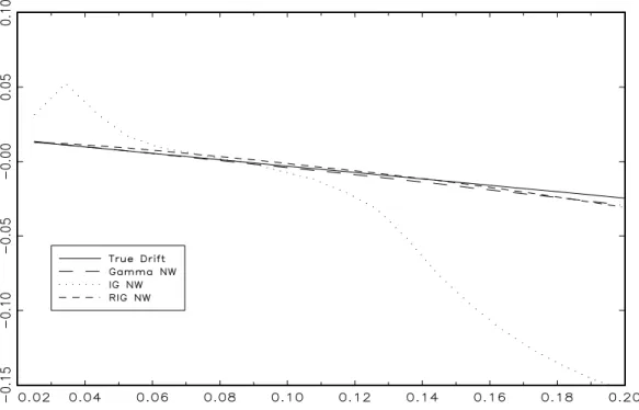
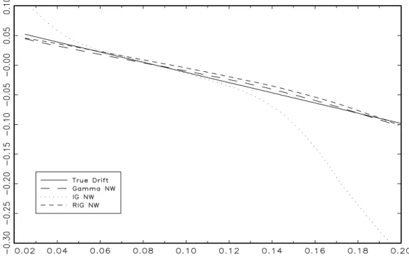
First, Figures 2 to 5 present the …nite-sample properties of the asymmetric NW estimators of the drift function from the CIR model. Figures 2 and 4 plot the median drift estimates of the Gamma, IG and RIG NW estimators for both parameterizations and a …xed smoothing parameter.

In agreement with the theoretical results in Section 2.2, the Gamma and RIG estimators exhibit very similar behavior and provide a very good approximation to the true drift function. In contrast, the IG drift function estimator is much more biased (the bias of the IG estimator is still substantial for larger smoothing parameters) and we do not consider this estimator further in the paper. Figures 3 and 5 plot the 90% Monte Carlo con…dence bands of the Gamma and RIG estimators and reveal that the Gamma estimator is less variable than the RIG estimator especially for the more persistent speci…cation. In the rest of the paper, we only report the results from the Gamma NW estimator noting that the RIG NW estimator delivers very similar results.

In order to compare the properties of the Gamma NW with the Gaussian NW, Gamma RNW and Gamma LL estimators, we choose a common algorithm for selecting the smoothing parameter based onh-block cross validation withh= 30(our experiments with di¤erent values ofhdelivered very similar results.) It is interesting to note that Gamma NW and RNW select signi…cantly smaller smoothing parameters than the Gaussian NW and Gamma LL estimators.

The median Monte Carlo estimates plotted in Figures 6 and 8 show that the Gamma NW and Gaussian NW are almost unbiased whereas the bias of the Gamma LL is rather large for both interior and boundary design points. It appears that the Gamma LL estimator is more sensitive to the high persistence in the data and its behavior improves for less persistent speci…cations. While the Gamma NW is only slightly less biased than the Gaussian NW, the asymmetric kernel estimator exhibits smaller variability (Figure 7) near the boundaries. The behavior of the asymmetric RNW estimator is similar to the Gamma NW estimator but it tends to be much more noisy.

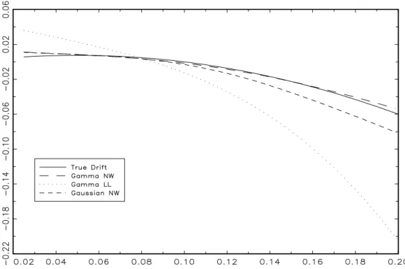
Finally, Figures 9 and 10 plot the drift function estimates from the nonlinear di¤usion speci…c-ation of Ahn and Gao (1999). As in the case of linear drift, the Gamma kernel estimator provides a very good approximation of the true drift function. The symmetric (Gaussian) NW estimator exhibits larger bias and variability for interest rates above 9% whereas the local linear estimator again tends to perform rather poorly compared to the asymmetric kernel estimator. In summary, the Gamma NW appears to be the best performing nonparametric estimator of the drift function of highly persistent di¤usion processes considered in the simulation experiments.

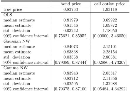
The economic signi…cance of the improved estimation of di¤usion models of spot rate is evaluated by comparing bond and option pricing errors based on di¤erent nonparametric estimators for the CIR model with ( ; ; ) = (0:21459;0:085711;0:0783). For reference, we include also the bond and option prices computed analytically from the OLS estimates of ; and obtained from the discretized version of the model. The results are presented in Table 1. Despite the fact that the OLS estimator uses knowledge of the true shapes of the drift and di¤usion functions, the bond and especially the call option prices are substantially underestimated due mainly to the severe downward bias of the OLS estimator in autoregressive models (Phillips and Yu, 2005). In contrast, the bond and derivative prices based on both symmetric and asymmetric kernel estimators are much less biased and actually produce slightly positive pricing errors. The bias of the Gamma estimator is smaller than its Gaussian counterpart but more importantly, the Gamma-based bond and option prices enjoy much smaller variability and tighter con…dence intervals than the symmetric kernel-based prices.

4

Conclusion

This paper proposes several asymmetric kernel estimators of conditional moment functions based on dependent data and nonnegative conditioning variables. The consistency, rate of convergence and asymptotic normality of these estimators are established for both interior and boundary design points. We show that the asymmetric kernel estimators possess some appealing properties such as lack of boundary bias and/or adaptability in the amount of smoothing. The paper adopts a block cross-validation method for dependent data in choosing the smoothing parameter. The …nite-sample performance of the estimators is evaluated in the context of a scalar di¤usion process of spot interest rate. Several interesting directions for future research include construction of bootstrap con…dence bands and bootstrap-based speci…cation testing, establishing uniform rates of convergence and rate improvement via multiplicative bias correction.

A

Appendix A: Proofs of Theorems

In this appendix, we present the proofs only for the Gamma kernel because the proofs for the IG and RIG kernels are similar. Note that approximations to the moments of the IG and RIG kernels can be obtained by following Scaillet (2004) and applying Lemmata B1 and B2.

A.1

Proofs of Theorems 1 and 2

The proofs of Theorems 1 and 2 require the following three lemmata. Before proceeding, de…ne t= (Yt) m(Xt).

Lemma A1. Let

ST = S0(x) b 1=2_S 1(x) b 1=2_S 1(x) b 1S2(x) :

If the conditions (A1)-(A5) hold, then for interior x,

SG;T _!p SG = 1 0 0 x f(x); SIG;T p !SIG = 1 0 0 x3 f(x); SRIG;T p !SRIG = 1 0 0 x f(x):

Proof of Lemma A1. Using Lemma B1,

E_fSG;j(x)g=E n (X1 x)jKG(x=b+1;b)(X1) o =En( 1;x x)jf( 1;x) o ; where 1;x d

=G(x=b+ 1; b). Taking a second-order Taylor expansion off( 1;x) around 1;x =x yields ( 1;x x)jf( 1;x) = ( 1;x x)jf(x)+( 1;x x)j+1f0(x)+ 1 2( 1;x x) j+2 f00(x)+Op n ( 1;x x)j+3 o :

Therefore, by Lemma B2, for interiorx,

E_fSG;0(x)g = f(x) +O(b);

E_fSG;1(x)g = ff(x) +xf0(x)gb+O b2 ;

Since strong mixing implies ergodicity, we can apply Birkho¤’s ergodic theorem to establish the results.

Lemma A2. Let

t_T = T0 (x) b 1=2_T 1 (x) = " T 1PT t=1 tKx;b(Xt) b 1=2_T 1PT t=1(Xt x) tKx;b(Xt) # :

Also for an arbitrary vector c₂ R2_{, de…ne Q}

T =c|tT. If the conditions (A1)-(A3), (A4’) and

(A5) hold, then for interior x,

V ar pb1=2_{T Q} G;T ! c|VGc=c| (" 1 2p x1=2 0 0 x1=2 4p # 2_(x)f(x) ) c; V ar pb1=2_{T Q} IG;T ! c|VIGc=c| (" 1 2p x3=2 0 0 x3=2 4p # 2_(x)f(x) ) c; V ar pb1=2_{T Q} RIG;T ! c|VRIGc=c| (" 1 2p x1=2 0 0 x₄p1=2 # 2_(x)f(x) ) c:

Proof of Lemma A2. It su¢ ces to demonstrate that

V arnpb1=2_{T T} G;0(x) o = 1 2p x1=2 2_{(x)f(x) +o(1); (7)} V arnpb1=2_{T b} 1=2_T G;1(x) o = x 1=2 4p 2_{(x)f(x) +o(1); (8)} Covnpb1=2_{T T} G;0(x); p b1=2_{T b} 1=2_T G;1(x) o = o(1): (9)

(i) Proof of (7). It follows fromE( tjXt) = 0that

V arnpb1=2_{T T} G;0(x) o = V ar ( 1 p T T X t=1 b1=4 tKG(x=b+1;b)(Xt) ) G;0(0) + 2 T_X1 j=1 1 j T G;0(j); (10) where _G;0(j) =b1=2_E

1 1+jKG(x=b+1;b)(X1)KG(x=b+1;b)(X1+j) is thejth-order autocovariance of the stationary process b1=4 tKG(x=b+1;b)(Xt) . For the …rst term on the right-hand side of (10), by the law of iterated expectations and Lemma B1,

G;0(0) = b1=2E n 2_(X 1)KG2(x=b+1;b)(X1) o = b1=2Ab;2(x)E 2( 2;x)f( 2;x) = b1=2 b 1=2_x 1=2 2p +o b 1=2 _E 2₍ 2;x)f( 2;x) ;

where 2;x=d G(2x=b+ 1; b=2). Taking a Taylor expansion of 2( 2;x)f( 2;x)around 2;x=xand using Lemma B2, we haveE 2₍

2;x)f( 2;x) = 2(x)f(x) +O(b)so that

G;0(0) =

x 1=2

2p

2_{(x)f(x) +o(1):}

On the other hand, for a constant a satisfying (A4’), pick a sequence d0T = b (1 2= )=(2a) . Then, the second term on the right-hand side of (10) is bounded by

T_X1 j=1 1 j T G;0(j) d0XT 1 j=1 G;0(j) + T_X1 j=d0T G;0(j) U1+U2:

ForU1, using t= (Yt) Ef (Yt)jXtgand the law of iterated expectations gives

G;0(j) b1=2 E E(j (Y1) (Y1+j)jjX1; X1+j)KG(x=b+1;b)(X1)KG(x=b+1;b)(X1+j) +E E(_j (Y1)jjX1; X1+j)E(j (Y1+j)jjX1+j)KG(x=b+1;b)(X1)KG(x=b+1;b)(X1+j) +E E(_j (Y1)jjX1)E(j (Y1+j)jjX1; X1+j)KG(x=b+1;b)(X1)KG(x=b+1;b)(X1+j) +E E(_j (Y1)jjX1)E(j (Y1+j)jjX1+j)KG(x=b+1;b)(X1)KG(x=b+1;b)(X1+j) b1=2_(U 11+U12+U13+U14):

As indicated in the proof of Lemma B2,G(x=b+ 1; b)has moments of any nonnegative integer order, and all these moments areO(1). Then, by (A2) and (A3),

U11 = Z 1 0 Z 1 0 E_{f j} (Y1) (Y1+j)jjX1=u; X1+j=vg KG(x=b+1;b)(u)KG(x=b+1;b)(v)f1;1+j(u; v)dudv c Z 1 0 Z 1 0 ( ₀+ ₁um+ ₂vn)KG(x=b+1;b)(u)KG(x=b+1;b)(v)dudv = O(1):

In addition, using (a conditional moment version of) Hölder’s inequality,

E_{f j} (Yt)jjXt=ug=Ef j (Yt) 1jjXt=ug E1=

n

j (Yt)j Xt=u

o

1:

Without loss of generality, assume 0 1 so that 0+ 1ul max

h

1; En_j (Yt)j Xt=u

oi

. Then, (A3) implies that

E_{f j} (Yt)jjXt=ug 0+ 1ul 1=

Using (11), (A2) and (A3), we have U12 = Z 1 0 Z 1 0 E_{f j} (Y1)jjX1=u; X1+j=vgEf j (Y1+j)jjX1+j=vg KG(x=b+1;b)(u)KG(x=b+1;b)(v)f1;1+j(u; v)dudv c Z 1 0 Z 1 0 ( ₀+ ₁um+ ₂vn) 0+ vl KG(x=b+1;b)(u)KG(x=b+1;b)(v)dudv = O(1):

Similarly,U13 O(1)can be shown. Furthermore, by (11) and (A2),

U14 = Z 1 0 Z 1 0 E_{f j} (Y1)jjX1=ugEf j (Y1+j)jjX1+j=vg KG(x=b+1;b)(u)KG(x=b+1;b)(v)f1;1+j(u; v)dudv c Z 1 0 0+ 1ul KG(x=b+1;b)(u)du 2 = O(1):

Hence, _G;0(j) O b1=2 _{, which establishes that}

U1 O d0Tb1=2 =O bfa (1 2= )g=(2a) !0:

ForU2, we can apply Davydov’s lemma (Corollary A.2 in Hall and Heyde, 1980) to obtain

G;0(j) 8f (j)g 1 2=

E b1=4 1KG(x=b+1;b)(X1) 2=

:

To …nd the bound forE b1=4

1KG(x=b+1;b)(X1) , note that since g(z) =z (z 0) is increasing

and convex, jx y_j (_jx_j+_jy_j) = 1 2 (2jxj) + 1 2 (2jyj) 1 2 (2jxj) + 1 2 (2jyj) = 2 1 _jx_j +_jy_j :

Substitutingx= (Y1)andy=Ef (Y1)jX1gyields

j 1j 2 1 h j (Y1)j +jEf (Y1)jX1gj i 2 1h_{j (Y} 1)j +E f j (Y1)jjX1g i : (12)

Then, we have E b1=4 1KG(x=b+1;b)(X1) cb =4 Z 1 0 En_j (Y1)j X1=u o K_G(x=b+1;b)(u)f(u)du + Z 1 0 E _{f j} (Y1)jjX1=ugKG(x=b+1;b)(u)f(u)du cb =4(U21+U22):

Again, as argued in the proof of Lemma B2, G( x=b+ 1; b= ) has moments of any nonnegative integer order and all these moments areO(1). Then, it follows from Lemma B1, (A2), (A3), and (11) that each ofU21 andU22 is bounded by

cAb; (x) Z 1 0 0+ 1ul KG(x=b+1;b=)(u)du OfAb; (x)g=O b(1 )=2 : Therefore,E b1=4 1KG(x=b+1;b)(X1) O b1=2 =4 , and thus U2 O b1= 1=2 T_X1 j=d0T f (j)_g1 2= O b (1 2= )=2 d_0Ta 1 X j=d0T ja_f (j)_g1 2= _!0; because O b (1 2= )=2 d_0Ta =O(1), d0T ! 1, and P1j=1jaf (j)g 1 2= < ₁. This completes the proof of this part.

Remark. We can demonstrate (7) even after replacing (A4’) by a weaker condition (A4). Observe that given (A4) andd0T = b (1 2=)=(2a) , each ofU1and U2still becomeso(1).

(ii) Proof of (8). We have

V arnpb1=2_{T b} 1=2_T G;1(x) o = V ar ( 1 p T T X t=1 b 1=4(Xt x) tKG(x=b+1;b)(Xt) ) G;1(0) + 2 T_X1 j=1 1 j T G;1(j); (13) where _G;1(j) =b 1=2_{E (X} 1 x) (X1+j x) 1 1+jKG(x=b+1;b)(X1)KG(x=b+1;b)(X1+j) is thejth -order autocovariance of the stationary process b 1=4_(X

t x) tKG(x=b+1;b)(Xt) . By the law of iterated expectations and Lemma B1, the …rst term on the right-hand side of (13) reduces to

G;1(0) = b 1=2E n (X1 x)2 2(X1)KG2(x=b+1;b)(X1) o = b 1=2Ab;2(x)E n ( 2;x x)2 2( 2;x)f( 2;x) o = b 1=2 b 1=2_x 1=2 2p +o b 1=2 _En₍ 2;x x)2 2( 2;x)f( 2;x) o ;

where 2;x=d G(2x=b+ 1; b=2). By a Taylor expansion and Lemma B2, we have En( 2;x x)2 2( 2;x)f( 2;x) o = xb+b 2 2 2_{(x)f(x) +O b}2 so that G;1(0) = x1=2 4p 2_{(x)f(x) +o(1):}

On the other hand, the second term on the right-hand side of (13) is bounded by T_X1 j=1 1 j T G;1(j) d1XT 1 j=1 G;1(j) + T_X1 j=d1T G;1(j) V1+V2;

where the sequenced1T is de…ned asd1T = b 3(1 2= )=(2a) for a constantasatisfying (A4’). For

V1, the same logic as in part (i) yields

G;1(j) b 1=2E Ef j (Y1) (Y1+j)jjX1; X1+jg jX1 xjKG(x=b+1;b)(X1) jX1+j xjKG(x=b+1;b)(X1+j) +b 1=2E E_{f j} (Y1)jjX1; X1+jg jX1 xjKG(x=b+1;b)(X1) E_{f j} (Y1+j)jjX1+jg jX1+j xjKG(x=b+1;b)(X1+j) +b 1=2E E_{f j} (Y1)jjX1g jX1 xjKG(x=b+1;b)(X1) E_{f j} (Y1+j)jjX1; X1+jg jX1+j xjKG(x=b+1;b)(X1+j) +b 1=2_{E Ef j (Y} 1)jjX1g jX1 xjKG(x=b+1;b)(X1) E_{f j} (Y1+j)jjX1+jg jX1+j xjKG(x=b+1;b)(X1+j) V11+V12+V13+V14:

Observe that by (A2), we havef 1_{(u) m} 1

1 so that f1;1+j(u; v) f(u)f(v) M2 m2 1 )f1;1+j(u; v) cf(u)f(v): (14) Using (A3), V11 cb 1=2 Z 1 0 ( 0+ 1um)ju xjKG(x=b+1;b)(u)f(u)du Z 1 0 j v x_jKG(x=b+1;b)(v)f(v)dv + Z 1 0 2 vn_jv x_jKG(x=b+1;b)(v)f(v)dv Z 1 0 j u x_jKG(x=b+1;b)(u)f(u)du cb 1=2(V111V112+V113V114):

The Cauchy-Schwarz inequality implies that V111 0 Z 1 0 (u x)2KG(x=b+1;b)(u)f(u)du+ 1 Z 1 0 um(u x)2KG(x=b+1;b)(u)f(u)du 1=2 Z 1 0 ( ₀+ ₁um)KG(x=b+1;b)(u)f(u)du 1=2 ( ₀V1111+ 1V1112)1=2V11131=2:

By a Taylor expansion and Lemma B2, we have V1111 = O(b) and V1112 = O(b). In addition,

V1113=O(1), and thusV111 O b1=2 . Similarly, each ofV112,V113andV114is at mostO b1=2 .

Hence,V11 O b1=2 . Applying the same procedure, we can also demonstrate that each ofV12,

V13 and V14 is bounded by O b1=2 . Hence, we can conclude that G;1(j) O b1=2 , which

establishes that

V1 O d1Tb1=2 =O bfa 3(1 2= )g=(2a) !0:

ForV2, we can apply again Davydov’s lemma to obtain

G;1(j) 8f (j)g 1 2=

E b 1=4(X1 x) 1KG(x=b+1;b)(X1) 2=

:

It follows from (11), (12), (14), and Lemma B1 that

E b 1=4(X1 x) 1KG(x=b+1;b)(X1) cb =4 Z 1 0 j u x_j En_j (Y1)j X1=u o K_G(x=b+1;b)(u)f(u)du + Z 1 0 j u x_j E _{f j} (Y1)jjX1=ugKG(x=b+1;b)(u)f(u)du cb =4Ab; (x) Z 1 0 j u x_j 0+ 1ul KG( x=b+1;b= )(u)f(u)du cb =4Ab; (x)V21:

By the Cauchy-Schwarz inequality,

V21 0 Z 1 0 j u x_j2 KG( x=b+1;b= )(u)f(u)du+ 1 Z 1 0 ul_ju x_j2 KG( x=b+1;b= )(u)f(u)du 1=2 Z 1 0 0+ 1ul KG(x=b+1;b= )(u)f(u)du 1=2 ( 0V211+ 1V212)1=2V2131=2:

V213=O(1), and thus we haveV21 O(b)so that E b 1=4(X1 x) 1KG(x=b+1;b)(X1) b =4O b(1 )=2 O(b) =O b3=2 3 =4 : Therefore, V2 O b3= 3=2 T_X1 j=d1T f (j)_g1 2= O b 3(1 2=)=2 d_1Ta 1 X j=d1T ja_f (j)_g1 2= _!0; becauseO b 3(1 2= )=2 _d a

1T =O(1), d1T ! 1, andP1_j=1jaf (j)g1 2= <1. This completes the proof of this part.

(iii) Proof of (9). We have

Covnpb1=2_{T T} G;0(x); p b1=2_{T b} 1=2_T G;1(x) o = Cov ( 1 p T T X t=1 b1=4 tKG(x=b+1;b)(Xt); 1 p T T X t=1 b 1=4(Xt x) tKG(x=b+1;b)(Xt) ) G;3(0) + 2 T_X1 j=1 1 j T G;3(j); (15)

where _G;3(j) = E (X1+j x) 1 1+jKG(x=b+1;b)(X1)KG(x=b+1;b)(X1+j) is the jth-order cross-covariance of the stationary processes b1=4

tKG(x=b+1;b)(Xt) and b 1=4(Xt x) tKG(x=b+1;b)(Xt) . By the law of iterated expectations and Lemma B1, the …rst term on the right-hand side of (15) reduces to G;3(0) = E n (X1 x) 2(X1)KG2(x=b+1;b)(X1) o = Ab;2(x)E ( 2;x x) 2( 2;x)f( 2;x) = b 1=2_x 1=2 2p +o b 1=2 _{E (} 2;x x) 2( 2;x)f( 2;x) ; where 2;x d

=G(2x=b+ 1; b=2). By a Taylor expansion and Lemma B2, we can see that

E ( 2;x x) 2( 2;x)f( 2;x) =O(b);

and thus _G;3(0) =o b1=2 _{=o(1). On the other hand, applying the same procedures as in parts}

(i) and (ii), we can also establish that the second term on the right-hand side of (15) iso(1). This completes the proof.

Lemma A3. If the conditions (A1)-(A3), (A4’), (A5)-(A6) hold, then for interior x, p b1=2_{T Q} G;T d !N(0;c|VGc);pb1=2_{T Q} IG;T d !N(0;c|VIGc);pb1=2_{T Q} RIG;T d !N(0;c|VRIGc):

Proof of Lemma A3. We employ the small-block and large-block argument. Partition the set

f1; : : : ; T_ginto2qT + 1 subsets with large block of sizerT and small block ofsT. Put

qT =

T rT+sT

:

Also let&_G;j =c|Z_G;j, where

Z_G;j = b 1=4 j+1KG(x=b+1;b)(Xj+1) b 1=4_(X j+1 x) j+1KG(x=b+1;b)(Xj+1) forj = 0; : : : ; T 1. Then, p b1=2_{T Q} G;T = 1 p T T_X1 j=0 &_G;j:

Furthermore, de…ne the random variables, for0 j qT 1,

G;j = j(rT+s_XT)+rT 1 i=j(rT+sT) &_G;i; _G;j= (j+1)(r_XT+sT) 1 i=j(rT+sT)+rT &_G;i; _G;q= T_X1 i=qT(rT+sT) &_G;i: It follows that p b1=2_{T Q} G;T = 1 p T 0 @ q_XT 1 j=0 G;j+ q_XT 1 j=0 G;j+ G;q 1 A p1 T (QG;T ;1+QG;T ;2+QG;T ;3):

We will show that

1 TE Q 2 G;T ;2 ! 0; (16) 1 TE Q 2 G;T ;3 ! 0; (17) E_fexp (itQG;T ;1)g qTQ1 j=0 E exp it _{G;j !} 0; (18) 1 T qXT 1 j=0 E _G;j2 _! c|VGc; (19) 1 T qXT 1 j=0 Eh _G;j2 1n _G;j (c|VGc)1=2 p Toi _! 0 (20)

for every > 0. (16) and (17) imply that QG;T :2 and QG;T ;3 are asymptotically negligible, (18)

and (20) are the standard Lindeberg-Feller conditions for asymptotic normality of QG;T ;1 under

independence. Hence, the lemma follows if we can show (16)-(20).

We …rst choose the block sizes. (A6) implies that a sequence _{T 2} N such that _{T ! 1}, TsT= b1=2T

1=2

!0, and _T T =b1=2 1=2 _(s

T)!0asT ! 1. De…ne the large-block sizerT by

rT =

$

b1=2_T 1=2

T

%

and the small-block size bysT. It follows that

sT rT ! 0; rT T !0; rT b1=2_T 1=2 !0; T rT (sT)!0 (21) asT _{! 1}. The proofs of (16)-(20) are given subsequently.

(i) Proof of (16). Observe that

E Q2_{G;T ;2} = q_XT 1 j=0 V ar _G;j + q_XT 1 i=0 q_XT 1 j=0; j6=i Cov _G;i; _G;j F1+F2:

ForF1, it follows from stationarity and Lemma A2 that

F1=qTV ar 0 @ sT X j=1 &_G;j 1 A=qTsTfc|VGc+o(1)g=O(qTsT): On the other hand,F2 can be further rewritten as

F2= qXT 1 i=0 qXT 1 j=0; j6=i sXT 1 l1=0 sXT 1 l2=0 Cov _G;mi+l1; _G;mj+l2 ;

where mj = j(rT +sT) +rT. Sincei 6= j, we have j(mi+l1) (mj+l2)j rT. Then, by stationarity, jF2j 2 T XrT 1 l1=0 T_X1 l2=l1+rT Cov _G;l1; _G;l2 2T T_X1 j=rT Cov _G;0; _G;j :

Note that the arguments used in the proof of Lemma A2 imply thatPT_j=r1_T Cov _G;0; _G;j =o(1). Therefore,_jF2j o(T), and thus, by (21),

1 TE Q 2 G;T ;2 =O qTsT T +o(1) =O sT rT +sT +o(1)_!0:

(ii) Proof of (17). Using a similar argument to the one used in the proof of (16), we have, by (21), 1 TE Q 2 G;T ;3 1 T fT qT(rT+sT)gV ar &G;0 + 2 T_X1 j=0 Cov _G;0; _G;j = o(1)_fc|VGc+o(1)_g+o(1)_!0:

(iii) Proof of (18). Observe that _G;a is _Fja

ia-measurable with ia = a(rT +sT) + 1 and

ja=a(rT +sT) +rT. Applying Lemma B3 withVj= exp it G;j and (21) yields

E_fexp (itQG;T ;1)g qTQ1 j=0 E exp it G;j 16qT (sT+ 1) 16 T rT +sT (sT+ 1)!0:

(iv) Proof of (19). By stationarity and Lemma A2, we have

E _G;j2 =V ar _G;j =rTfc|VGc+o(1)g: Therefore, by (21), 1 T q_XT 1 j=0 E _G;j2 =qTrT T fc |_VGc+o(1)g rT rT +sT c|VGc_!c|VGc:

(v) Proof of (20). We employ a truncation argument because j is not necessarily bounded. Let L_j = j1fjjj Lgfor some …xed truncation pointL >0. Also let&G;jL =c|ZG;jL, where

Z_G;jL = b 1=4 L j+1KG(x=b+1;b)(Xj+1) b 1=4(Xj+1 x) Lj+1KG(x=b+1;b)(Xj+1) : Furthermore, de…ne QG;TL = 1 b1=4_T T_X1 j=0 &G;jL; G;jL = j(rT+s_XT)+rT 1 i=j(rT+sT) &G;iL:

In addition, let~&G;jL =c|Z~G;jL, where

~ Z_G;jL = b 1=4_~L j+1KG(x=b+1;b)(Xj+1) b 1=4_(X j+1 x) ~Lj+1KG(x=b+1;b)(Xj+1)

and~L_j = j1_fj jj> Lg. Finally, de…ne

~ Q_G;TL = 1 b1=4_T T_X1 j=0 ~ &_G;jL so thatQ_G;T =Q L G;T + ~QG;TL .

Since bothKG(x=b+1;b)(u)anduKG(x=b+1;b)(u)are bounded above, we have

(Xj+1 x)KG(x=b+1;b)(Xj+1) <1 (22)

forj = 0; : : : ; T 1 so that & L

G;j cLb 1=4. Then, L G;j cLrTb 1=4; (23) and thus, by (21), L G;j p T c rT p b1=2_T !0: It follows that Prn L G;j (c|VGc) 1=2p To= 0 (24)

at allj for su¢ ciently largeT. Then, applying (23) and (24), we have

1 T qXT 1 j=0 Eh _G;jL 21n _G;jL (c|VGc)1=2 p Toi c prT b1=2_T 2q_XT 1 j=0 Prn _G;jL (c|VGc)1=2pTo_!0:

In other words, (20) holds for the truncated variables. Consequently, we have the following asymp-totic normality result

p b1=2_{T Q}L G;T = 1 p T T_X1 j=0 &_G;jL _!d N 0;c|VLGc ; (25) whereVL G=V ar ZG;jL Xj=x .

The remaining task for establishing (20) is to show that as …rstT _{! 1}and thenL_{! 1},

b1=2T V ar Q~_G;TL _!0: (26) Indeed, Enexp itpb1=2_{T Q} G;T o exp t 2 2c |_VGc Enexp itpb1=2_{T Q} L G;T o exp t 2 2c |_VL Gc + E n exp itpb1=2_TQ~ L G;T o 1 + exp t 2 2c |_VL Gc exp t2 2c |_VGc E1+E2+E3:

By (25),E1 ! 0 as T !0 for everyL > 0. E3 !0 as …rst T ! 1 and then L! 1, because

VL_{G !} V ar Z_G;j Xj=x =VG by the dominated convergence theorem. We can also see that

E2!0as …rstT ! 1and thenL! 1, if (26) holds. Now,

lim

T!1b

1=2_{T V ar Q~} L

G;T =c|V ar Z~G;jL Xj=x c=c|V ar ZG;j1fjjj> Lg Xj =x c!0 asL_{! 1}by the dominated convergence theorem. This completes the proof.

A.1.1 Proof of Theorem 1 Lemma A3 implies that

p b1=2_T ( 1 T T X t=1 KG(x=b+1;b)(Xt) t ) d !N 0; 2_(x)f(x) 2p x1=2 : Also, de…ne ~ mnwG (x) = PT t=1KG(x=b+1;b)(Xt)m(Xt) PT t=1KG(x=b+1;b)(Xt) =S_G;1₀(x) ( 1 T T X t=1 KG(x=b+1;b)(Xt)m(Xt) ) :

Then, by the de…nitions ofm^nw_G (x)and t,

^ mnw_G (x) m~nw_G (x) =S_G;1₀(x) ( 1 T T X t=1 KG(x=b+1;b)(Xt) t ) :

Therefore, by Slutsky’s lemma and Lemma A1, we have

p b1=2_Tfm^nw G (x) m~nwG (x)g d !N 0; 1 2p x1=2 2_(x) f(x) : (27)

In addition, a second-order Taylor expansion yields

~ mnw_G (x) =m(x) +m0(x)S_G;1₀(x)SG;1(x) + m00_(x) 2 S 1 G;0(x)SG;2(x) +OpfSG;3(x)g; (28) where SG;1(x) =ff(x) +xf0(x)gb+op(b); SG;2(x) =xf(x)b+op(b); SG;3(x) =Op b2 (29)

by Lemma B2 and the ergodic theorem. Substituting (29) into (28) and using Lemma A1 and (A7), we can see that the left-hand side of (27) can be approximated by

p b1=2_Tfm^nw G (x) m~nwG (x)g = pb1=2_{T m^}nw G (x) m(x) m0(x) 1 + xf0_(x) f(x) + 1 2xm 00_{(x) b+o} p(b) = pb1=2_{T m^}nw G (x) m(x) m0(x) 1 + xf0_(x) f(x) + 1 2xm 00_{(x) b +o} p(1):

This completes the proof. A.1.2 Proof of Theorem 2

Lemma A3 and the Cramér-Wald device imply that pb1=2_Tt

G;T d

! N(02;VG), where 02 is the

2 1 zero vector. Also, de…ne

~ G(x) = ( 1 T T X t=1 KG(x=b+1;b)(Xt) 1 Xt x 1 Xt x ) 1( 1 T T X t=1 KG(x=b+1;b)(Xt) 1 Xt x m(Xt) ) :

Then, by the de…nitions of^G(x)and t,

1 0 0 b1=2 n ^ G(x) ~G(x) o = 1 0 0 b 1=2 1( 1 T T X t=1 KG(x=b+1;b)(Xt) 1 Xt x 1 Xt x ) 1 ( 1 T T X t=1 KG(x=b+1;b)(Xt) 1 Xt x t ) = 1 0 0 b 1=2 1( 1 T T X t=1 KG(x=b+1;b)(Xt) 1 Xt x 1 Xt x ) 1 1 0 0 b 1=2 1 1 0 0 b 1=2 ( 1 T T X t=1 KG(x=b+1;b)(Xt) 1 Xt x t ) = S_G;T1 t_G;T:

Therefore, by Slutsky’s lemma and Lemma A1, we have

p b1=2_T 1 0 0 b1=2 n ^ G(x) ~G(x) o _d !N 02;S_G1VGS_G1 : (30)

In addition, a second-order Taylor expansion yields

~ G(x) = (x) +m00(x) 2 1 0 0 b 1=2 SG;T1 1 0 0 b 1=2 SG;2(x) SG;3(x) + OpfSG;3(x)g Op b 1SG;4(x) (31); where SG;2(x) =xf(x)b+op(b); SG;3(x) =Op b2 ; SG;4(x) =Op b2 (32)

by Lemma B2 and the ergodic theorem. Substituting (32) into (31) and using Lemma A1 and (A7), the left-hand side of (30) can be approximated by

p b1=2_T 1 0 0 b1=2 n ^ G(x) ~G(x) o = pb1=2_T 1 0 0 b1=2 ^G(x) (x) m00_(x) 2 xb Op(b) + op(b) Op(b) ; where pb1=2_{T o} p(b) = op p b5=2_{T = o} p(1), and p b1=2_{T b}1=2_O p(b) =b1=2Op p b5=2_{T = o} p(1). Therefore, (30) can be rewritten as

Tb;1 ^G(x) (x) 1 2xm00(x)b 0 + op(1) op(1) d !N 0 0 ; 1 0 0 1 2x VG by lettingTb;1= p b1=2_T 1 0 0 b1=2 , andVG= ₂p1_x1=2 2_(x)

f(x). This completes the proof.

A.2

Proof of Theorem 3

The proof of Theorem 3 requires the following three lemmata. Before proceeding, we introduce some additional notation. For interiorx, de…ne

bG;t(x) = 1 + 4p 1 x1=2 + x1=2f0(x) f(x) b 1=2_(X t x)KG(x=b+1;b)(Xt) 1 ; bIG;t(x) = 1 + 4p x3=2 f0_(x) f(x)b 1=2_(X t x)KIG(x;1=b)(Xt) 1 ; bRIG;t(x) = 1 + 4p x1=2 f0_(x) f(x)b 1=2_(X t x)KRIG(1=(x b);1=b)(Xt) 1 :

For suchbt(x)depending on a particular asymmetric kernel Kx;b(u), let

J1= 1 p T T X t=1 b1=4bt(x) tKx;b(Xt):

Lemma A4. If the conditions (A1)-(A5) hold, then for interior x,

V ar(JG;1)! 2_(x)f(x) 2p x1=2 ; V ar(JIG;1)! 2_(x)f(x) 2p x3=2 ; V ar(JRIG;1)! 2_(x)f(x) 2p x1=2 :

Proof of Lemma A4. It follows from (22) thatbG;t(x) = 1 +op(1). Then, applying the same arguments which are used to establish (7), we obtain the stated results.

Lemma A5. Let Wj(x) = 1 T T X t=1 (Xt x)jKx;bj (Xt); j2N:

If the conditions (A1)-(A5) hold, then for interior x,

WG;1(x) = ff(x) +xf0(x)gb+op(b); WG;2(x) = x1=2_f(x) 4p b 1=2_+o p b1=2 ; WG;3(x) =Op(b); WIG;1(x) = x3=2f0(x)b+op(b); WIG;2(x) = x3=2_f(x) 4p b 1=2_+o p b1=2 ; WIG;3(x) =Op(b); WRIG;1(x) = xf0(x)b+op(b); WRIG;2(x) = x1=2f(x) 4p b 1=2_+o p b1=2 ; WRIG;3(x) =Op(b):

Proof of Lemma A5. Using Lemma B1,

E_fWG;j(x)g=E n (X1 x)jK_Gj_(x=b+1;b)(X1) o =Ab;j(x)E n ( j;x x)jf( j;x) o ; where j;x d

=G(jx=b+ 1; b=j). Taking a second-order Taylor expansion and using Lemma B2, we have, for interiorx,

E_fWG;1(x)g = EfSG;1(x)g=ff(x) +xf0(x)gb+o(b); E_fWG;2(x)g = Ab;2(x) xb+b2 2 f(x) +O b 2 ₌ x1=2f(x) 4p b 1=2_{+o b}1=2 _; E_fWG;3(x)g = Ab;3(x)O b2 =O(b):

Finally, the ergodic theorem establishes the results.

Lemma A6. If the conditions (A1)-(A5) hold, then for interior x,

G = G(x) = 4p 1 x1=2 + x1=2_f0_(x) f(x) b 1=2 f1 +op(1)g; IG = IG(x) = 4p x3=2 f0_(x) f(x)b 1=2 f1 +op(1)g; RIG = RIG(x) = 4p x1=2 f0(x) f(x)b 1=2 f1 +op(1)g;

so that pt(x) = T 1bt(x)f1 +op(1)g for bt(x) depending on a particular asymmetric kernel

Kx;b(u).

Proof of Lemma A6. It follows from (22) that we can pick some constantMG >0 such that

sup

0 j T 1

Then, applying expression (6.4) in Chen and Hall (1993) and using Lemma A2, we have

j Gj j

WG;1(x)j

jWG;2(x)j MGjWG;1(x)j

=Op b1=2 :

Furthermore, a second-order Taylor expansion of the right-hand side of

0 = 1 T T X t=1 (Xt x)KG(x=b+1;b)(Xt) 1 + G(Xt x)KG(x=b+1;b)(Xt) around G= 0gives 0 =WG;1(x) GWG;2(x) + 2 GWG;3(x)

for some Gjoining Gand0. Since Gis a convex combination of Gand0, we have G=Op b1=2 so that 2_GWG;3(x) =Op b2 by Lemma A5. Therefore, substituting the results in Lemma A5 yields

G= WG;1(x) WG;2(x) + 2_GWG;3(x) WG;2(x) = 4p 1 x1=2 + x1=2_f0_(x) f(x) b 1=2 f1 +op(1)g+Op b3=2 ; andpG;t(x) =T 1bG;t(x)f1 +op(1)g by (3).

A.2.1 Proof of Theorem 3 It follows from Lemma A6 that

^ mrnw_G (x) m(x) = PT t=1f (Yt) m(x)gpG;t(x)KG(x=b+1;b)(Xt) PT t=1pG;t(x)KG(x=b+1;b)(Xt) b1=2T 1=2JG;1+JG;2 J_G;1₃f1 +op(1)g; where JG;2 = 1 T T X t=1 fm(Xt) m(x)gbG;t(x)KG(x=b+1;b)(Xt); JG;3 = 1 T T X t=1 bG;t(x)KG(x=b+1;b)(Xt):

To approximateJG;2, note that

1 T T X t=1 (Xt x)2KG(x=b+1;b)(Xt) =SG;2(x) =xf(x)b+op(b):

Then, taking a second-order Taylor expansion and using (2) andbG;t(x) = 1 +op(1), we have

JG;2 = 1 T T X t=1 m00_(x) 2 (Xt x) 2 bG;t(x)KG(x=b+1;b)(Xt) +OpfSG;3(x)g = 1 2xm 00_(x)f(x)b+o p(b):