Proposing Logical Table Constructs for Enhanced
Machine Learning Process
MUHAMMAD FAHIM UDDIN 1, (Student Member, IEEE), SYED RIZVI2, (Member IEEE), AND ABDUL RAZAQUE3, (Senior Member, IEEE)
1Department of Computer Science, School of Engineering, University of Bridgeport, Bridgeport, CT 06604, USA 2Department of Information Science and Technologies, Penn State University, Altoona, PA 16601, USA 3Department of Computer Science, New York Institute of Technology, New York, NY 11568-8000, USA
Corresponding author: Muhammad Fahim Uddin ([email protected])
This work was supported by the School of Engineering, University of Bridgeport, Bridgeport, CT, USA.
ABSTRACT Machine learning (ML) has shown enormous potential in various domains with the wide
variations of underlying data types. Because of the miscellany in the data sets and the features, ML classifiers often suffer from challenges, such as feature miss-classification, unfit algorithms, low accuracy, overfitting, underfitting, extreme bias, and high predictive errors. Through the lens of related study and latest progress in the field, this paper presents a novel scheme to construct logical table (LT) unit with two internal sub-modules for algorithm blend and feature engineering. The LT unit works in the deepest layer of an enhanced ML engine engineering (eMLEE) process. eMLEE consists of several low-level modules to enhance the ML classifier progression. A unique engineering approach is adopted in eMLEE to blend various algorithms, enhance the feature engineering, construct a weighted performance metric, and augment the validation process. The LT is an in-memory logical component, that governs the progress of eMLEE, regulates the model metrics, improves the parallelism, and keep tracks of each module of eMLEE as the classifier learns. Optimum fitness of the model with parallel ‘‘check, validate, insert, delete, and update’’ mechanism in3-Dlogical space via structured schemas in the LT is obtained. The LT unit is developed in Python, C#, and R libraries and tested using miscellaneous data sets. Results are created using GraphPad Prism, SigmaPlot, Plotly, and MS Excel software. To support the built and implementation of the proposed scheme, complete mathematical models along with the algorithms, and necessary illustrations are provided in this paper. To show the practicality of the proposed scheme, several simulation results are presented with a comprehensive analysis of the outcomes for the metrics of the model that the LT regulates with improved outcomes.
INDEX TERMS Big data, predictive modeling, data mining, machine learning, algorithm, parallel processing of machine learning metrics reading, model tuning, algorithm blending, optimum fitting, feature engineering, overfitting,eMLEE, logical table.
I. INTRODUCTION A. BACKGROUND
Machine learning (ML)unveils tremendous potential in the data science and predictive analytics.MLalgorithms partic-ularly in the supervised learning (SL) zones have advanced into improved modeling of the underlying data for decision making [1], predictive analytics [2], personality prediction [3] etc. Great surveys such as [4]–[6] including domains of the unstructured data [7] and social networking platforms have shown incredible importance of ML algorithms’ tun-ing and improvements [8]. Useful techniques such as algo-rithm boosting [9], optimization [10], conditional densities, gradient descent, inference [11], parallel processing [12],
and convex minimization have played progressive roles to improve the classifier learning of the existing tech-niques inSL.
The latest progress in the research of data mining and predictive modeling with the relevance ofMLhave promoted great opportunities and challenges for future works. Prior to developing the work presented in this article, we investigated the application ofMLtechniques reported in the literature. We found high relevance in the areas of healthcare domain applications to predict hospital admissions [13], [14], practi-cal applications to deal with lethal diseases such as HIV [15], and biomedical device applications [16]. Other areas included security, facial recognition, engineering solutions,
and general modeling such as antenna design opti-mization [17], image classification [18], and real-world experiences such as driver safety [19], and algorithm optimization [20], [21].
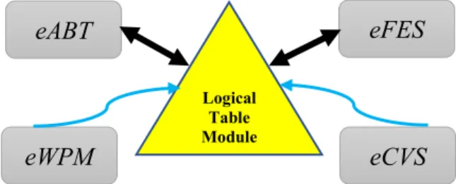
Therefore, considering the progresses outlined above, and the literature study provided in Section II, we see the necessity of introducing a parallel processing unit in theML underlying models. The diversity in the data and features have motivated us to improve the latest state ofMLmodels by building enhancedMLengine engineering (eMLEE) pro-cess specially to address the challenges such as overfitting, underfitting, bias, low accuracy, poor generalization, and pre-dictive errors. While the details ofML engine engineering (i.e., eMLEE) is beyond the scope of this article, LT con-structs are presented. LT is a vital component of eMLEE. As shown in Fig. 1,eMLEEis composed of four modules. The triangular shape emphasizes on the idea of3Dconcept that the model operates on. The thick arrow betweeneFES, eABT,andLTmodule shows core integration than the other two modules ofeMLEE. The major modules ofeMLEEare enhanced Algorithm Blend and Tuning (eABT) and enhanced Feature Engineering and Tuning (eFES) that are regulated by LTinternal unit.
FIGURE 1. This illustration shows the elevated system externals of eMLEE.LTinteracts witheFESandeABTon the deeper level. It coordinates and regulates the metrics of the learning process in parallel mode.
eMLEEmodel is based on parallel processing and learns from its mistakes (i.e., processing and storing the wrong predictions). Its modules are, i) enhanced algorithm blend and tuning (i.e.,eABT) to optimize the classifier performance, ii)enhanced feature engineering and selection(i.e.,eFES) to optimize the features handling,iii) enhanced weighted per-formance metric (eWPM) to validate the fitting of the model, andiv)enhanced cross validation and split (eCVS) to tune the validation process. Out of these, eCVS is at infancy of the research work. Existing research, as discussed inSection II has shown the limitations of general purpose algorithms inSL for predictive analytics, decision making, and data mining. Thus,eMLEEfinds its place to fill the gaps that Section II discusses.
Finally, LT is built to coordinate the internal flow of eMLEEas introduced briefly in the above paragraph.
B. MOTIVATION AND NOVELTY
The motivation to develop this specialized unit comes from the uniquely thought, experimented, developed, and
incorporated parallelism in an enhanced machine learning process with innovative blending and tuning as discussed earlier.eMLEEcomes in to addressing ‘‘No Free Lunch the-orem’’ problem, feature correlation, and selection improve-ment. It addresses challenges such as overfit, underfit, bias, predictive errors, and poor generalization. In our experi-mental tests during the evolution of this research, we felt the necessity of ‘‘inline’’ unit as a centralized part of this engine that governs, regulates, and keeps track of machine learning process on the underlying data. The challenge of trade-off between vital metrics such as complexity, accu-racy, speed, etc. becomes also very important and that is whereLT plays a significant role. LT creates parallel pro-cess for each element in each run governed by 3D object co-ordinates (x,y and z) and then makes observations in the real time of classifier learning and updates its logical row in the table. This approach is novel to the best of our survey and knowledge.
C. CONTRIBUTIONS
Below are the contributions of the work presented in this article.
i. The in-memory processing unit is designed and gov-erned by algorithms, that ensures the model internals are at maximum performance during blend.
ii. A blended model such as eMLEE will use LT unit to tune the performance metrics in the real-time. This feature is built using mathematical constructs. iii. The 3D logical modeling is used to reserve x
(under-fitting), y (over(under-fitting), and z (optimum-fitting). Algo-rithms are written to score each dimension during the learning process. 3D improves the visualization pro-cess during simulations.
iv. LT also is needed to teach the model to learn from its mistakes. However, this contribution is left for another article that elaborates deeply on eABT unit.
v. Improves the trade-off between various metrics such as complexity, speed, accuracy etc., using real-time evalu-ation and locating the optimized point for each element using 3D visualization and recording techniques. vi. Finally, LT unit is structured as a centralized
com-ponent of blended model, for keeping coordina-tion between each component regulated with built-in parallel processing.
D. PARALLELISM
As stated earlier,LT regulateseABT andeFES. LTplays a key role to introduce an effective parallelism (i.e., parallel processing) ineMLEEengine. Here we summarize the par-allel processing of the engine that incorporates theLTunit, as centralized and vital component of the system for the proposed enhanced machine learning process.
i) Outer layer to eABT, where eABT unit communi-cates with other units of the eMLEE such as eABT, eWPM, eCVSandLT. Parallelism is done through real time metrics measurement with LT object. Based on
classifier learning, eABT reacts in the inner layer (defined next). Other units such as eFES and eCVS enhance the feature blend and test-training split in par-allel, whileeABTis being trained. In other words, all four units includingeABTregulated byLTunit, are run in parallel to improve the speed of the learning process and validation for the blend as processed ineABTunit. However,eABT can also work without being related to the other units, if researchers and industrialists may however choose so.
ii) Inner layer toeABT, where addition and removal of the algorithm are done in parallel. When the qualifying algorithm is added, the metrics are measured by the model to see if fitness improves, and then algorithms are added or removed one by one to see the effect on the fitness function. This may be done sequentially, but parallelism improves the insurance that each algorithm is evaluated at the same time, the classifier is incor-porating metrics reading fromLTobject and speed of the process improves, especially when a huge dataset is being processed.
E. SIMULATION STRATEGY AND RESULTS PRODUCTION
We provided detailed information about our data sources and tools in Appendix. Because our research investigated the ensembling of algorithms (that learn based on different classifier curves), we considered a very miscellaneous set of training and testing data to ensure that our blend of algo-rithms stay in the optimum fitting range for the real-world experiments and analytics. Similarly, because of the feature engineering and tuning, it was authoritative to our work using data with assorted set of features involved.
We also uniquely adopted the following approaches to make our experiments more reliable, easy to interpret, repro-duce, and analyze for the model’s validation, integrity and evaluation.
1. We conducted 100’s of experiments to cover wide range of datasets that helped achieved in-depth training of the model to study various ranges of metrics. We then re-evaluated our math constructs and algorithms to improve fitness. This way, our math constructs gov-erned by our algorithms, ensured the integrity of the model through the lens of real-world data and testing. 2. We also sampled all these experiments and
devel-oped a novel approach of 10-experiemntal rule. This way, we could present our outcomes and analysis with improved visualization and interpretation, as presented in this article.
We used Python and R data analysis packages along with C# libraries to test our algorithms. We used Prism, SigmaPlot, and Excel to produce our simulated results. We uniquely adopted the approach of3Dto have more observational value to our analysis for the proposed model. This article reports preliminary results in3Dmodeling and matured results in2D modeling of the simulations runs for the experiments we have conducted.
F. PAPER ANATOMY
The rest of the article is structured as follows. Section II discusses the related study that supports the contribution of eMLEEengine, the part of which is the LT, as proposed in this article. Section III & IV discuss the theory, algorithms, illustrations, and simulated results of the LT contructs for eABTandeFES respectively. Section V presents simulated and experimental results for theLTunit in depth. Section VI concludes with final remarks. Appendix and references are provided at the end.
Key Notations:
II. RELATED STUDY
Brief related study is provided in the areas ofML. This explo-ration of the literature helped and promoted our contribution of theLTfor enhancedMLsuch aseMLEE.
Tuia et al. [22] provided a survey of active learning algorithms in the field of remote sensing image classifica-tion. Mainly focused onSVMalgorithm, they discussed the issue of efficient training set, having high impact on the expected outcome. Their findings, results, and discussion
showed that active learning algorithms are making great progress especially for image classification and the type of data it involves. However, their contribution was limited to active learning, especially for image classification and may not be suitable to apply for a diverse set of data and fea-tures. Garcia et al. [23] provided a survey on discretization techniques with empirical analysis in supervised learning. Discretization is an important approach specially to improve the underlying algorithm in terms of feature/attribute tuning and qualitative analysis. They provided in-depth analysis and guidelines of various methods with taxonomy table of their findings. Their findings also suggested an ideal selection of a method for given problem. Their findings and exper-iments showed accuracy of various MLtechniques but did not provide other metrics that may be of special interest especially when blend is being engineered for a greater gen-eralization. Wang et al. [24] discussed the process of pur-chase decision in subject minds usingMRIscanning images through ML methods. Using recursive cluster elimination basedSVMmethod, they obtained higher accuracy (71%) as compared to previous findings as per their research. They utilized Filter (GML) and wrapping methods (RCE) for fea-ture selection. Their work though provided great foundation and motivation for feature processing but did not provide the in-depth experiments of application of the technique on neutral subjects where feature may mislead, and algorithm design must take this into account. Tandon et al.[25] dis-cussed the importance of machine intelligence in big data domain towards natural language. Their work provided great motivation towards mining common sense that can extracted from words of people, but it did not provide in-depth analysis of algorithms or features that may impact such intelligence during learning process. Hernandez et al. [26] discussed the parallel processing optimization in big data applications. Their results showed improved recommendations score for resources and workload but did not address or consider the parallel processing of various algorithms to see if that could further improve their work. Dai and Song [27] work was focused on multiple classifier systems (MCSs) with their con-tribution of supervised competitive learning algorithm (SCL) to improve the accuracy of the classifiers. Though their work showed satisfactory progress for accuracy measurements, did not consider other metrics of the supervise learning classifier especially if algorithm blend is intended.
Some of the work in the areas of engineering domains such as antenna design, wireless communication, chip designs and other biomedical engineering are using advancedML tech-niques with recent availability of digital data. Liuet al.[17] addressed the low efficiency of evolutionary algorithms in Electromagnetic(EM) design problems due to the cost, and thus proposed a new method called surrogate model differ-ential evolution for antenna synthesis usingMLtechniques. Their work was very limited to EM applications and did not provide the wide applicability to other domains of sim-ilar challenges in EM or Electrical engineering domains. Yu et al. [28] focused on weaknesses of semi-supervised
clustering algorithms and to address these challenges, they proposed closure based constraint approach and random bases semi-supervised framework. They used datasets from medical domains such as cancer patients. Their work lacks dealing with pairwise constraints and removal of redun-dant constraints. Such limitation may be addressed by the work in the feature optimization and engineering as we propose. Xiao-jian et al. [29] advanced the work in opti-mization extreme learning machine (OELM) for the error penalty parameter C. Their work extended the traditional OELM classifier with the regularized parameter v. Their work created useful foundation for classifier parameter opti-mization. However, they lacked to confirm the stability of optimization if different classifiers were used or tested. Lara and Labrador [30] provided a survey onMLapplication for wearable sensors, based on human activity recognition. They provided a taxonomy of learning approach and their related response time on their experiments. Their work also supported feature extraction as an important phase of ML process. Their work provides great motivation for feature engineering and further improvement in feature selection and optimization. Vergara and Estevez [31] reviewed fea-ture selection methods. Authors presented updates on results in unifying framework to retrofit successful heuristic crite-ria. The goal was to justify the need of feature selection problem in-depth concepts of relevance and redundancy. However, their work lacks to address the issues of model fitting when a diverse set of features are involved in datasets. Mohsenzadehet al. [32] utilized a sparse Bayesian learning approach for feature sample selection. Their proposed rele-vance sample feature machine (RSFM), is an extension of RVM algorithm, previously invented. Their results showed the improvement in removing irrelevant features and pro-ducing better accuracy in classification, better generalization, less system complexity, reduced overfitting and computa-tional cost. Maet al. [33] utilized Particle Swarm Optimiza-tion (PSO) algorithm to develop their proposed approach for detection of falling of elderly people and enhance the selec-tion of variables (i.e., hidden neurons, input weights, etc.) Their experiments showed higher sensitivity, specificity, and accuracy readings. Their work lacked to consider various algorithms in comparison withPSOto see if it might impact the modeling of the various metrics.
The following points highlight the weaknesses/gaps out-lined by the related study and our in-depth literature review.
a) Algorithm and Feature blending for various algorithms are at infancy state in the research work published and applied, and thus lack lots of improvements, such as incorporating each algorithm and feature for maximum accuracy possible.
b) Algorithms are not taught to learn from their mistakes and thus LT is needed to fill this gap.
c) Hidden features, that can be of great predictive value are often overlooked and thus LT can improve this gap. Similarly, research related to the removal of irrelevant and redundant features are rarely found.
d) A real-time optimization functions are rarely imple-mented in other models, when the model learns and may fail to fit. LT, however works in-parallel during training and testing process to fill this gap.
e) Finally, general-purpose algorithms, such as LT, are not implemented where new modules like eABT or eFES can be extended to the existing models, such eMLEE. III. LT THEORY OF eABT MODULE
LTas previously discussed, is a vital central unit ofeMLEE. LTis based on3Dnovel concept of optimization to regulate the metrics and learning progress of the blended model. In this section, we first discuss each definition in plain English and then provide the details of building theLTunit mathematical constructs in conjunction with algorithm definition.
A. DEFINITIONS IN PLAIN ENGLISH
Definition 1covers the theory of Adder and Remover func-tions for the3Dobjects formulation based on the progress of blend of algorithms and features incorporation as the clas-sifier learning continues. This way each element is cross-checked in parallel and metrics readings are recorded as a new logical row or updated as existing row.
Definition 2 covers the theory of specialized factors for LTunit based on fitness of the classifier learning. These are used to construct a vital function known as scoring function that quantifies each factor for3Devaluation and identifying signal and noise in the dataset for further optimization.
Definition 3covers the theory of specialized function as Error Boundto support rule of optimum fitness. This intro-duces a novel concept for error regulation in the proposedLT model. Staying between 20 % and 80 % ensures that model never over or under learns the data. This has been proved to be an effective approach in the results being observed by our study and work.
Definition 4 covers the theory of two vital functions/ constructs:i) Blending, and ii) Tuning function. These con-structs turned out to be very useful for classification goals. This definition also constructs the Binary Decomposition function thatLTobject uses to formulate and determine the cost function.
Definition 5covers the detailed theory ofCost function based onDef. 4.This cost function plays another vital role to evaluate the comparing elements in the algorithms and features and compute the accurate quantification of blending and tuning functions.
B. MATHEMATICAL CONSTRUCTION OF THE UNIT’ INTERNALS
LT operates in the memory and is dynamically updated. It keeps tracks of the algorithms A(x,y,z) = {A1,A2, . . .
. . . ,An,} as the ML process evolves to accomplish the final optimum fitting after it has incorporated all the algo-rithms from the pool. This helps achieve the optimum blend-ing and tunblend-ing. LT stores data based on three dimensions, where ‘x’ = over-fitness, ‘y’ = under-fitness and ‘z’ =
optimum-fitness. In our model, we will be using ‘‘-ness’’ to
mathematically phrase the metric for modeling purposes. At this stage, we refer fitness to be the overall performance of the model, and our goal is to reduce ‘x’ and ‘y’ to as minimum as zero and improve ‘z’ to the highest possible value. ‘R’
is the ratio between the single error from an algorithm and averaged error of all the algorithms in the blend.’ Ne1 ‘is the normalization factor for the error‘err’.‘Err’indicates the Overall error determined for the blended model.
Let us define constant error function: kx,y,z=
1
p
2πµ3
+ReABT (1)
Where,µcomputes all the values ofx,y, and zcomponents during learning. µ = 1 N N X i=1 (x,y,z)i (2) ReABT = 1 Ne r err err+Err 2 (3)
Definition 1: Let there be a Adder Function as ‘AddFunc(A(x,y,z))’, that adds each algorithm in the blend being processed, with Scoring Function as ‘ScoFunc(0:1)’ for each dimension in 3D space. Let there be a Remover Function as ‘RemFunc(∗), that must hold at-least one element per each test.∗indicates the computed dimension.
LTstructure uses the grouping and scoring module. Scor-ing is based on binary number weights as beScor-ing illustrated in Fig. 5 and based on the following rule.
Rule 1 If (LTObject.ScoFunc(A(i)>0.5) Then Assign ‘‘1” Else Assign ‘‘0” LT(x,y,z)= 1 if LT.ScoFunc>0.5 0 if LT.ScoFunc<0.5 ?Undetermined (4)
By combining Gauss-Markov and Chebyshev methods [34] we construct adder FunctionLas given by
AddFunc=(An∪An+1) "Q LT>0.5A(z) BIN(min(x,y) # (5) Our rule of thumb was 0.5 or 50 % to see how the model learns. This way, we can separate the zone of over learn-ing and under learnlearn-ing from a border line of 50 %. Once classifier learns the zoning limits, it will decide this number itself. Q
LT>0.5
A(z) acts a regulating factor that provides the continuous product for each value ofz-dimensionfor which theBINfunction returns the least possible value ofxandy.
The removing function is —given by RemFunc(∗)=(An∩An+1) "Q LT<0.5A(x,y) BIN(max(x,y) # (6)
It is imperative to validate the Adder and Remover func-tions at this point, using well known technique ofFrobenius norm[35]form: kMk(x,y,z) =kx,y,z v u u u t X X x=1 Y X y=1 Z X z=1 M2 x,y,z(AddFunc,RemFunc) (7)
WhereM shows the matrix and we will elobrate on it in the later section.
Definition 2: Let Op.F, Un.F, Ov.F, and Bias.F be the factors for Optimum-fitting, Underfitting, Overfitting, and Bias respectively of the algorithm under test in 3D model. There must be an equal random distribution for each till LT regulates the scoring function (SF) for each metric.
Each metric swings from {0:1} based on the correla-tion of algorithm during each test. LT object receives the score for each element while classifier learns in3D space. Dimentionality reduction and multivariate classification tech-niques [36] can be used to construct a function for LT, as shown in (8) and (9), LT(z)=ltElement× lim z>0.5 {SF(Op.F)} (8) SF(x,y,z)=LT(z)− X X i=1 Y X j=1 LT(i,j) (9) ltElementshows the object forLTsuch aseABT. LTobject creates an entry in the memory for tracking the metrics for each element such as a particular algorithm under test, and it assigns the weights (binary based) to each metric as per in definition 2, for which the following is constructed:
PROCEDURE 1
Execute LT.ScoreMetrics(Un.F, Ov.F) Compute LT.Quantify(*LT)
Execute LT.Bias(Bias.F, *)
*_Shows the pointer to the LT object.
Clearly, the noise in the data (i.e., the irrelevant or redu-dant) does not have good predictive value, thus the metrics stated in the definition 2 are highly affected by it. We build a loss function in correspondent to Noise (N) and Signal (S) (i.e., data of predictive value). Thus, we construct our binary loss function, based on our rule of thumb from the signal and noise for the training.
L(DS(S(x,y,z),N(x,y,z)
= (
0,&(N(x,y,z)≥0.5≥S(x,y,z))
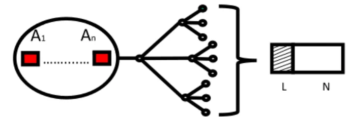
1,&(S(x,y,z)≥0.5≥N(x,y,z)) (10) Not likely but loss function tends to get very unstable in a blend or 2+algorithms where classifier function has a very low variant and probability of distribution of fitness function across z-axis (i.e. fitness model) is very wide. Thus gener-alization ability of the net model becomes very significant. The 3-branch diagram inFig 2. shows the spread of algorithm in each dimension, that corresponds toLandN component. An example is shown in rectangular shape for L and N
FIGURE 2. Illustration of Loss and Noise interoperation based on x, y, and z dimensions, for algorithms blend.
co-variance, for algorithms blend. Each small circle repre-sents the occurrence of a big circle on the left.
Definition 3:Let lt.Err be the specialized error function that implements the rule of optimum fitness (RoOpFit) as 0.2<lt.Err<0.8. Every entry in LT must adhere to this rule.
Rule 2
Except random errors, lt.Err must be regulated to stay in between 20 to 80 % to avoid over and under learning. If lt.err < 0.2
Then : Label it ‘Overlearning’
Elseif lt.err > 0.8
Then:Label it ‘underlearning’
From the literature, we can implement the RMSE function for error determination, thus, we use our rule to build:
max(e:0.8) = 1 E Ne X i=1 {(RMSEi)−(100+0.2)/E} (11) min(e:0.2) = 1 E Ne X i=1 {(RMSEi)−(100+0.8)/E} (12)
Using (11,12), we build theRoOpFitto lead towards deter-mination oflt.Errfunction.RoOpFitregulates the error that LT object can trigger for each test. Using kernel density function [36] and margin limits in Lipschitzness [9], we build
RoOpFit =max err <0.8 x,y X i,j (Ai,j)−min err >0.2 y,x X j,i (Aj,i) (13) lt.Err(x,y,z) = Y RoOpFit(z) − Y RoOpFit(z) BIN((x,y,z) (An) (14) With this error function being constructed, we can easily see the divergence in the optimum zone of z-axis. As dis-cussed before, the LT object reads the previous entry and then based on the data from the training blend classifier, it updates (i.e., writes or deletes) in its logical structure (i.e., new or existing row of records).
Definition 4:LetBAn be a blending function andTAn be a tuning function that LT object must compute (detailed in algorithm definition). Let BIN((x,y,z))be a binary decom-position function for each entry in LT. There must exist a Cost function as ‘C’.
In SL, the classifier function Classifier(1S(x,y,z)) =
1 N as identified, where 1S = i1,o1 , i2,o2 , . . . . . . . ik,ok
and for regression: Errorsok ∈RFor Classification:okis a
discrete value. In Linear Classification, as generally done in SVMconcept: we can use Lagrange multipliers [37] to present the problem in equivalent maximization onγ :
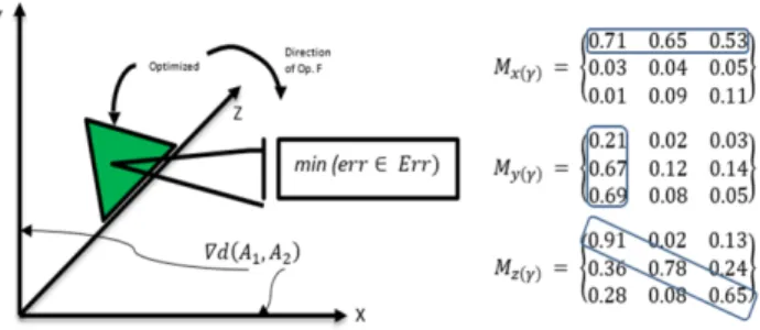
γ =argmaxXN k=1γk− 1 2 XN k,l=1γkγl(okol <ik,il >) (15) InFig 3, triangle is lying on z-axis, with the direction of momentum as being engineered in the model.∇d shows the Euclidean distance between two algorithms under test. The three Matrices shown are typical values for the sampling of the several hundred experiments. The encircled values show the optimized value of each axis for the desired optimization as LT object stores and reports.
FIGURE 3. – Illustration of optimum fitness logical(x, y, z)triangle.
Equation (16) shows that Blend function is composed of three parts that work on AddFunc, RemFunc and score for each algorithm in each dimension as LT computes (See Algorithm 1 definition). Using Regularization in local minima where error is minimum but lipschitz loss [9] is unknown, we use vector product to keep the uniformity at minimum random distribution such that z 6= 0 AND x, y<0.5, thus, we construct BAn(0:1)= AddFunc(k) Y k=1 Ak× xk yk zk + RemFunc(m) Y m=1 −Ak× −xm −ym +zm (16)
Tuning function is constructed usingErranderrfunctions. As we stated earlier theRoOpFmust be followed for blend to be tuned for improved optimization. LT object ensures by recording and manipulating the metrics, as per algorithm structure, discussed later. Thus, we can write:
TAn(0:1)= 1 N N X i=1 −(BAn)−
((Err−(Err+err)
2)
(17)
Definition 5:There must exist a cost function as ltCost, that must adhere to the minimum distance required between two algorithm during test, in logical space for ltCost(x,y,z),
FIGURE 4. Illustration ofBAn(Blue),TAn(Red) as it theoretically spread in
optimum space of x, y, z dimensions.
for which the condition ltCost(00,z)∈1(Distance(x,y,z)> 0, always exist.
During recognition of hidden patterns or points in datasets, the loss or cost function (C):
C(f (i:input) ,o:output))
= 1
2|f (i)−o|, ik ∈I, ok ∈O (18) LTis built on three constructs:i) to monitor and store the ratioReABT,ii)to update the values ofx,y, and zcomponents
of each algorithm classifier during training, andiii)to score the algorithm An| {0:1},n ∈ (N +1), using Blending
FunctionBAn(0:1), and Tuning FunctionTAn(0:1). LT.eABT =ReABT × N X n=1 An(f(x,y,z) exp BAn BAn+TAn (19)
Fig. 4shows three adjacent visual concepts. Our goal is to optimize the Blending and Tuning function withLTobjects such that, it corresponds to high convergence in z-dimension.
Fig. 4 shows three examples of such cases, that may be expected throughout experimental observation with the real-world data. As shown in theFig. 5, the values are updated based on the function that we built using simple linear regres-sion, so when we fit a line on the given points, we can estimate the linearity of the classifier that is being built by the model as more algorithms are blended (governed byBAn(0:1)) and
then tuned (governed byTAn(0 : 1)). We must incorporate
the squared error as [(mxk+a)−yk]2, which translates to
difference between true value and predicted value, Thus:
T(m,a)=kx,y,z. K X
k=1
[(mxk+a)−yk]2 (20)
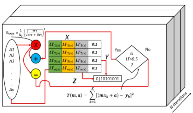
Fig. 5shows the internal mechanics of theeABT LT work-ing model. It is internally based on binary classification tech-nique. As the logical table grows with the quantized output as explained above, it decides which algorithm is a good fit in the blended model. As we can observe, thatLT governs the process at the lowest level of the model being proposed. It creates the entry for each dimension(X, Y, and Z)as shown. As a threshold, if theLTvalue is less than 0.5, it is assigned binary ‘0’, and if it is>0.5, it is assigned binary ‘1’. Based on this, the binary truth table is built, and is used in the algorithm 1.
Algorithm 1Algorithm 1LT −eABT LT Governance
Goals:It governsLTstructure in the memory to keep track of fitness of the model, for algorithm blend.
Input:A.P = {A1,A2,A3, . . . ..,An}/∗ the algorithms pool for improving generalization∗/
Output:NODESi∈N, eABT
Initiate:Create data libraries object asObjDS, ObjLT 1: Set:x,y,z←ObjDS.RandomValues(0)
2:While(0.2<err ∈Err<0.8)Do
3: Compute: error constant using equation (1) 4: Set: µ← 1 N N P i=1 (x,y,z)i
5: Compute:ReABT using equation (3)
6: For(each ObjLT.Evaluate(1) inz)Do
7: Set: z←0
8: Compute:T(m,a)using equation (20) 9: Set:γ ← 1 2ln 1−εt ε
10: Update: Probability of Hypothesis: 11: Ht :I → {−1,+1}
12: If(Pt+1(k) <0.5)Then
13: Set:Errt ←Pk:Ht(ik)6=okPt(k)
14: Read: ObjDS.Evaluate(Errt,γ)
15: Pt+1(k)← PtZt(k)× ( e−γt IfHt(ik)=ok eγt IfHt(ik)6=ok 16: Compute: ObjLT.Write(Pt+1(k)) 17: Else
18: Set:Errt ←ObjLT.Read(Ht, γ)
19: Update: ObjLT.Update(err, Err)
20: End If
21: Set: A(x,y,z)← (1x+1),(1y+1),(1z+1) 22: Compute:ERM(3D)
23: Compute: Add/RemFunc based on eq (5,6) 24: Write: ObjLT.Write(ERM(3D))
25: End For
26: Compute: ObjLT.FitnessScore(A(i)) 27: Update: ObjLT.Update(err(z), Err(z)) 28: For(each node inNODESi∈N)Do
29: If(Score(Ai∈ A(i+1))>node(i))) Then 30: Update: ObjLT.Zscore(ObjDs,Az)
31: Read: ObjLT.Read(score(z))
32: End If
33: Set: Next node
34: End for
35: Compute: BAn /∗Using Equation (16)∗/ 36: Compute:TAn /∗Using Equation (17)∗/ 37: Update: ObjLT.eABT(BAn,TAn)
38: End While
39: Return: eABT
Based on illustration inFig. 5, we can build our Blending and Tuning Functions for the LT using in-parallel binary weight distribution for each algorithm.
Next, we build our empirical risk minimization(ERM) function based on error-probability function, so we can then
FIGURE 5. Illustration ofeABTLogical Table Internals.
TABLE 1.Tuning and blending function typical observation.
TABLE 2.Observance of error functions in typical ratios.
optimize the fitness space (3D) usingLT to logically con-vert (i.e., move overfitting and underfitting to optimum fitting space) the invalid fitness score to which algorithm resists to learn. Error scores are used to measure the degree of success for an element (such as algorithm) to participate in group for the blend, especially in the interest of optimum fitting’s. Thus, we define the following rules:
Rule 3
Pr(err)∼x→ (y(i)6=z(i))
Rule 4
Pr(err in z(i)∼z→(x(i+1)6=(y+1)
On the most inner layers of the learning, the errors can be considered in two types: training errors and testing error, thus, to score theERM, we can assume
ERM(err(train,test))= ( −erm, err(z)<0 erm, err(z)≥0 (21) By definition: ERM(3D)= | i∈[n]:3D(di)6=(d+1)i | n (22) Where [n]={1,2,3,4. . . .,N}
Inductive bias and hypothesis (h) class are used to rectify the problem of overfitting in ERM [35]. Inductive bias is
considered a set of restrictions where we bias the hypothesis class towards a predictor that will not overfit and thus, we can minimize its effect.
ERM(h)∈argmin h∈H
ERM(3D) (23)
C. ALGORITHM DETAILS AND DEFINITION
In this section, we provide complete definition ofLT Algo-rithm foreABTmodule. This algorithm uses two important libraries:
i) ObjDS, for general dataset sources in raw or formatted shape including what Python or R packaged offer, and
ii) ObjLTis an object of theeMLEE API, forLTmodule to access the function written for its working. The following definition is written in standard format for ease of implemen-tation using standard languages and packages.
Algorithm pool (A.P) represents the3Darray in the mem-ory that stores the pointers for each dimension ofx,y, and z. Based on the scoring mechanism explained earlier, it holds the computed values for each algorithm (SLalgorithms) as they are brought into, for testing (Algorithm’eABTinternal layers). Along with other functions, in conjunctions with Algorithms as defined next, finally the optimum SL algo-rithms are identified and weighted accordingly for classifier blending.
The main while loop atstep 2makes sure that rule 2 is obeyed. Steps 3-5 compute error functions and Ratio as constructed in the math model. The firstForloop atstep 6
ensures the optimum fitness is regulated in the z-dimension.
Steps 7-12 build the probability distribution hypothesis so the cost function is decentralized for improved labelling of each element in each row asLTobject receives it.Ifblock at
step 13checks and maintains the probability of the fitness to be greater than 50 % for more training to be continued and then we update theLT objects.Step 26sets the changes in each dimension for the algorithm element being incorporated and then updates the global object.In steps 26-28, we com-pute ERM function and use equation 5&6 to utilize adder and remover function. Insteps 31 to 39, we update theLTobjects for all theMLalgorithms incorporated (added or removed) based on the desired fitness and error ranges as per rules defined in the module.Steps 40-45finally compute the blend-ing and tuner functions as we constructed in the mathematical model and return the quantized data to the calling function of the algorithm object.
Fig. 6shows that it is based on binary weighted classifica-tion scheme to identify the algorithm for blending and then assign a binary weight accordingly inLTlogical blocks. The diamond shape shows the err distribution that is observed and recorded byLTmodule as new algorithm is added or existing is removed.
The illustrations shown in Fig. 7,8,9 are the result of 20-experimental run for over 3000 data samples in our lab environment for evaluatingLTmodule ineMLEE infras-tructure. The simulation uses four colors. Blue, to indicate extreme overfitting in each dimension. Green and yellow
FIGURE 6. This illustration shows the concept ofLTmodular elements in 3-Dspace as discussed earlier.
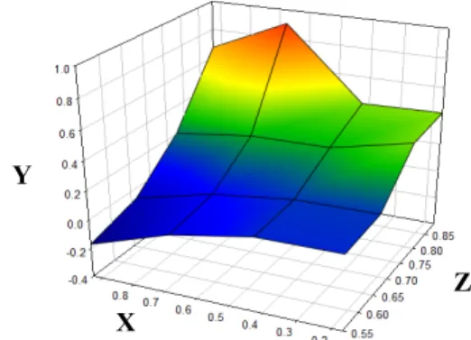
FIGURE 7. It shows theLToptimum fitness ability in each dimension. We noticed error at the negative value.
FIGURE 8. This shows the ideal behavior of theLToptimum fitness function. As we see, the blue section is virtually absent. And it further elaborates that z-dimension has the maximum convergence of the function, as ideally desired.
show that classifier was not able to distinguish between underfitting and overfitting, and orange color shows the opti-mum fitting.
IV. LT THEORY OF eFES MODULE
Very similar to constructs we built foreABT LT unit, this logical table also operates in the memory and is dynami-cally updated. It keeps tracks of the features F(x,y,z) = {F1,F2, . . . ,Fn,}as the ML process evolves to accom-plish the final optimum fitting after it has tried all the features from the pool. Similarly, it also stores data based on three dimensions, where ‘x’=under-fitness, ‘y’=over-fitness and ‘z’=optimum-fitness. Features in the given datasets are of
FIGURE 9. This is the real (experimental) behavior of Figure 8.
several types. They are also known as ‘attributes’ or ‘vari-ables’. Type includes:i) numeric, such as continuous values such as time, speed, height and weight or discrete such as age, counts, and ii) categorical such as Gender, Color, Race, and Ranks. Some of the categories of features are linguistic, structural, and contextual.
In this section, we first discuss each definition in plain English and then we provide the details of building the LT module mathematical constructs and provide algorithm definition.
A. DEFINITIONS IN PLAIN ENGLISH
Definition 6 covers the theory for Adder and Remover
function likeDef. 1but for feature engineering as the second layer ofLTunit.
Definition 7covers the theory of function that quantifies
the score of each feature as it is introduced in the dataset so the correlation can be improved and decentralized.
Definition 8as the last theoretical foundation builds the
Irrelevant and Redundant functions so the scoring of each feature can be done row-wise for each test of the classifier learning. This way, the model learns to determine the opti-mized predictive value of each feature, as a part of feature engineering and optimization that LT object governs and handles. This way, the right numbers and type of features set is created.
B. MATHEMATICAL CONSTRUCTION OF THE UNIT INTERNALS
Definition 6: Let there be two functions, Feature Adder as+F, and Feature Remover as−F, based on linearity of the classifier for each feature under test for which the RoOpF is valid (as described in Definition 3), and a feature is not repeated in the group.
eFES LTmodule builds very important functions at initial layers for adding a good fit feature and removing a bad fit feature from the set of features available to it, especially when algorithm blend is being engineered. Clearly, as we discussed, not all features will have optimum predictive value and thus identifying them will count towards optimization. The feature
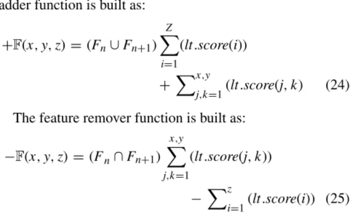
adder function is built as:
+F(x,y,z)=(Fn∪Fn+1) Z X i=1 (lt.score(i)) +Xx,y j,k=1(lt.score(j,k) (24) The feature remover function is built as:
−F(x,y,z)=(Fn∩Fn+1) x,y X j,k=1 (lt.score(j,k)) −Xz i=1(lt.score(i)) (25) Very similar to k-means clustering [38] concept, that is highly used in unsupervised learning,LTimplements feature weights mechanism(FWM) so it can report a feature with high relevancy score and non-redundant in a quantized form. Thus, we define: FWM(X,Y,Z) = X X x=1 Y X y=1 Z X z=1 (uxwx.uywy.uzwz)(1(x,y,z)) (26) 1 (x,y,z) = L Y l=1 (ulxwlx), if z6=0, AND z>(0.5,y) ui∈ {0,1}, −1≤i≤L L Y l=1 (ulywly), if z6=0, AND z>(0.5,x) (27)
Definition 7:Let there be a Feature Scoring Function as FScore in LT module for which the correlation between each feature as accepted is minimum. Let Cor(x,y,z) be a function to compute the score for the feature sets as grouped in the LT object.
FScore(x,y,z)and Cor(x,y,z)are functions on the second layer that ensure each entry is recorded in theLTobject as the process continues. We build,
FScore(x,y,z)= Z Di (Fi|X,Y,Z)pidVx,y,z (28) Cor(x,y,z)= H(fi)−H(fi|fi+1) H(fi+1−H(fi+1|fi) H(fi)+H(fi+1)−H(fi,fi+1) (29) PROCEDURE 2
Import Features: a finite number of features Set F in n > 0, Integer T >0
Initialization: Define the categorical or
numerical values, and set F(n) = Constant value For F = {F1,F2,F3, ...,Fn,}
Select F(n) based on random function and define the distribution in space, D[f(T)|F(n)]∈
∂ F(F(n))
Update each f ∈ F(n), for which fn ≥ F{0.85,0:1} is valid
FIGURE 10. This test shows the variance of the LT module for the cost function for all three co-ordinates and then z (optimum-fitness). This is the ideal behavior.
FIGURE 11. This test shows the real (experimental) behavior.
FIGURE 12. Demonstration to illustrate the entropy-based feature distribution in space based on binary system.
Fig. 12shows two colors (yellow and green) for same func-tion related to each feature (i) and (i+1). Thus, the entropy function is calculated in the inner layer of LT object as the features are added or removed based on matching scoring function.
Definition 8: Let lt.IrrF and lt.RedF be two functions to store the irrelevancy and redundancy score of each fea-ture for a given data set in LT object and then correlates it for each test in blend of algorithms using lt.BlendAlgo Function, such that each feature obeys the condition0.3 > lt.BlendAlgo(lt.IrrF,lt.RedF) >0.7}.
To constructIrr.FandRed.F, we implement Markov Blan-ket method in which we apply sequential filters to remove the feature one by one for higherRed.F and Irr.F. We alter the values between {−1 to+1) for theoretical consideration.
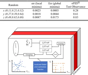
TABLE 3.Observance of error functions in typical ratios.
FIGURE 13. Illustrates of the N-experimental iteration of the conceptual flow.
It must be noted, that the values between {0 to 1} are realistic and mathematically possible. We build a mutual informa-tion (MI) function [31] so we can quantify the relevance of a feature upon other in the random set. This information is used to build the construct forIrr.F, as the classifier learns, it will mature the Irr.F learning module as defined in the algorithm1. MI(Irr.F(x,y,z)|fi,fi+1) = N X a=1 N X b=1 p(fi(a) , fi+1(b) .log fi(a) , fi+1(b) p(fi(a) .fi+1(b) (30) Irr.F = K X i,j fii fij fji fji =
MI(fi;Irr.F) >0.5 Strong Relevant Feature MI(fi;Irr.F) <0.5 Weak Relevant Feature MI(fi;Irr.F)=0.5 Neutral Relevant Feature
(31)
We use the (31) to develop the relation of ‘Irr.F’andMI to show the irrelevancy factor and redundant factor based on binary correlation and conflict. Redundancy is another impor-tant quantity to compute for feature correlation, especially in classification problems. We use Markov Blanket [31], [39] to make the following assumptions, ss ⊆ ¬fi is Markov
Blanket, if
p({F{fi,ss}|{fi,(x,y,z)})=p({F{fi,ss}|{fi}) (32) Fig. 13illustrates theN-experimental iteration of the con-ceptual flow shown. As we can observe, thatLTgoverns the process at the lowest level. It creates the entry for each dimen-sion(X, Y, and Z).As a threshold, if theLTvalue is less than 0.5, it is assigned binary ‘0’, and if it is>0.5, it assigns ‘1’.
FIGURE 14. This illustrates the ideal outcome of eFES LT fitness function in 3D space. Notice the z-axis has the least blue color.
This shows the mechanics of the logical design of the algo-rithm being proposed. It shows that it may takeNnumber of iterations to tune the table function. As discussed earlier,LT keeps track of the feature engineering for optimum fitting and outlier detection for a model being trained. Threshold is set to 50 % forLTfunction return value. This shows that as features are added, theLTstays above 0.5, or features may need to be removed. The two-dimensional figures in Fig. 13(with blue and orange lines) demonstrate the underfitting and overfitting as the model encounters and reports back to theLTobject.
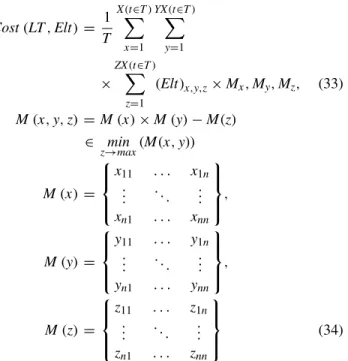
Finally, we build our cost and matrix function as follows:
Cost(LT,Elt)= 1 T X(t∈T) X x=1 YX(t∈T) X y=1 × ZX(t∈T) X z=1 (Elt)x,y,z×Mx,My,Mz, (33) M(x,y,z)=M(x)×M(y)−M(z) ∈ min z→max(M(x,y)) M(x)= x11 . . . x1n ... ... ... xn1 . . . xnn , M(y)= y11 . . . y1n ... ... ... yn1 . . . ynn , M(z)= z11 . . . z1n ... ... ... zn1 . . . znn (34)
Equation (34) supports the functionality ofFig. 7. Next, we defineLT algorithm foreFES module. The information related to accessing common libraries have been stated in the opening remarks of algorithmLT-eABTalready in the earlier section.
C. ALGORITHM DETAILS AND DEFINITION
In this section, we provide detail ofeFES LTalgorithm based on the mathematical model and associated libraries.
FIGURE 15. This illustrates the real(experimental) analysis of the test, we performed on validationeFESmodule.
FIGURE 16. This test shows the three metrics (Underfitting(UF), Overfitting (UF), and optimum-fitting (OpF) for 500 experimental-run. LTmodule successfully identified and process the features that contribute to each metric accordingly.
FIGURE 17. This test shows the matching function built ineFESalgorithm for random vs correlated data points. As we observed, it shows the promising behavior (expected) when it is highly correlated than just the random test.
Step 1initializes the optimum fitness factor.Step 2begins thewhileloop to check for Ratio that is governed by local and global errors correlation, so the function remains in-bounds of over-learning and under-learning logical3Dspace.Steps 3-4
compute the global Error and hypothesis function for even probability distribution as discussed in the mathematical model.Step 5starts theForloop to evaluate each feature and quantifiesx,y, and zas it spreads in space using3Dlogical elements, so the row can be updated accordingly.Steps 20-23
compute the Ratio function so the local error can be regulated and then update the LT object in the library call. Then it resets each co-ordinate for next run in the loop.Steps 24-28
build the references for computing Feature Adder and Feature Remover function for feature grouping function using LT parallel evaluation technique as explained earlier in the model build of Section 4. In Steps 29-33, theIfblock checks for each algorithm entry so the Ratio can be re-calculated and this way, theNo Free Lunch Theoremproblem is also addressed. Finally steps 34-38compute the main eFES function after updating the central probability function, so the bias can be minimized for each feature before adding to the group. Then in last step, the function reference is returned to the calling pointer of the algorithm.
PROCEDURE 3
For (each node in tree) Do
Execute: Add Function for new element Update each node for maximum points
If (t <= 0.5~in absolute T) Then Read next node
Move to next node in tree and add the previous node to the LT Object
End If
Set: x,y and z values from node to LT object Update LT
Execute the Algorithm~LT eABT
While (there are more algorithms to test) Do
Compute the CF for each algorithm Run the optimization test as shown in~Figure~18
Update the results Find new~(t) t++ (increment) Update x,y, and z End While
Execute Algorithm~LT eFES For (each feature in the set) Do
Execute the Adder and Remover function Find new~(t)
t-- (decrement) Update the CF Function End For
End For
With the results shown for eABTandeFES LTmodules in the lowest level of eMLEEinfrastructure, we show our low-level framework for theLT mechanism inFig. 18. We first develop the cost function for each node as shown in the illus-tration for each dimension in 3-Dlogical space. As shown that z can vary from 1 to n values depending upon how many iterations will it take to achieve the optimum fitting of the model withLTobject.t∈T indicates all the values of tuning function in the unit terms during training ofLTobject. These values can vary both in negative and positive because LT object keeps track of both underfitting and overfitting of the model in its logical layers and rows.
V. RESULTS AND ANALYSIS A. EXPERIMENTAL SETUP
The various datasets were used to improve the generalization of the model. The details of datasets are listed in Appendix. Datasets were divided in three sections, as a standard prac-tice,i) Train, ii) Test, and iii) Validation. However, we also uniquely split the data (as defined in the algorithm) governed by the real-time metrics using LT object. In this process,
Algorithm 2LT–eFES Logical Table Governance
Goals:It governsLTstructure in the memory to keep track of fitness of the model.
Input:A.P = {A1,A2,A3, . . . ..,An}/∗ the algorithms pool for improving generalization∗/ Raw Feature Set F(x, y, z) = {F1∈Fn}
Output:NODESi∈N,eFES
1: Set:{Op.F ←0,F(x.y,z)←(0,0,0)} 2:While((ReABT)<(r(e+E))Do 3: Compute:Errt ← P k:Ht(ik)6=ok Pt(k) 4: Compute: Hypothesis:Ht :I → {−1,+1} 5: For(# of F in Set)Do 6: Set: γ ← 1 2ln 1−ε t ε
7: Compute: x,y, and z for ObjLT.Random 8: Update: ObjLT.Update(x,y,z,γ) 9: If(γ <(γ −1))Then
10: Set:γ ← (γ +1) 11: Read: ObjLT.Read(x,y,z) 12: Compute: :Pt+1(k)← PtZt(k)
13: Else
14: Set:γ ← (γ −1)
15: Update: ObjLT.Update(x,y,z,γ)
16: End If 17: Compute:ReFES← N1 e q e e+E 2
18: Update: ObjDS.Update(ReFES,ObjLT)
19: Set:x←(x+1) ,y←(y+1) ,z← (z−1)
20: End For
21: Write: ObjDS.Write(x,y,z, ObjLT) 22: Compute:+F/∗Using equation (24)∗/ 23: Compute:−F/∗Using equation (25)∗/ 24: Update: Scores for each algorithm, and 25: creates NodesNODESi∈N
26: For(each node inNODESi∈N)Do
27: If(SCORE(Ai∈ A(i+1))>node(i)) Then 28: Add: entry to LT 29: Re-compute:ReABT 30: Update: LT 31: End If 32: Finally Update:Pt+1(k) 33: Compute: eFES(x,y,z)←
34: ObjLT.Optimize(ReABT,BAn,TAn)
35: End While
36: Return:NODESi∈N, eFES
the random slices of data were created and then they were flipped to elevate the predictive errors temporarily. This way, LTobjects learn on maximum possible errors and then tune itself (i.e., algorithm) to improve the slice in the next run and so on. This is also supported inLTmathematical model (i.e., Definitions). This also chains the ideas of enhanced validation and parallelism as we stated in the Introduction section.
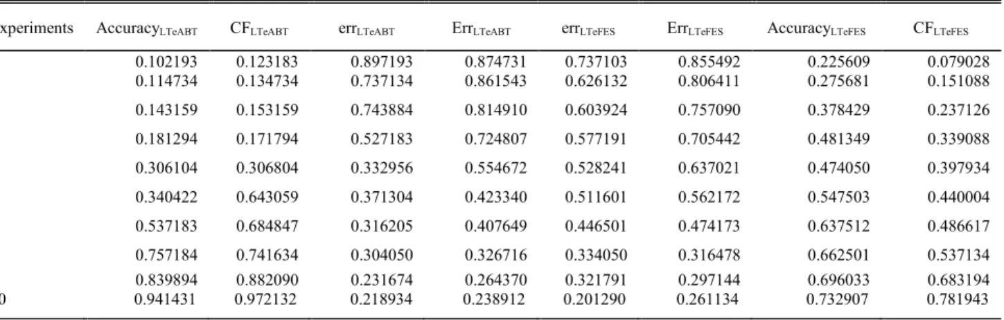
TABLE 4. LTmetrics foreFESandeABT.
FIGURE 18. LT framework at low-level.
Validation datasets split tested how well the model was learning (i.e., learned skill) and testing datasets substantiated the bias of the model, as it learned. In main model ofeMLEE several ML algorithms such as Support Vector Machines, Decision trees, Logistic Regression, Multiple Linear Regres-sion, Bayes networks, etc., were used to test the model via the blending mechanism (i.e., eMLEEinternals). However, the eMLEEunderlying proposed algorithms, outside of the scope of this article, allow researchers to incorporate any supervised learning algorithm of their choice, to overcome the challenge of ‘‘No Free Lunch theory’’ as we discussed in the introduction section. That is the beauty and novelty of this model based onLT. We have used existing libraries of Python and R scientific packages on the exact datasets
TABLE 5.X observations.
TABLE 6.Y observations.
TABLE 7.Z observations.
that we setup for our experiments so we could draw com-parison charts and record tabular data. However, the compar-ison details ofeMLEEare also outside of the scope of this paper.
Appendix lists the details of the libraries we have used to implement the mathematical model and algorithm as pro-posed in the article. However, end users are free to use the language of their choice to build it.
B. RESULTS PRESENTATION AND DISCUSSION
Table 4 lists the average outcome of 10-experimental process that was adopted as a part of the experimental validation of the constructs. Several experiments were performed on a diverse set of data to improve the generalization of the model
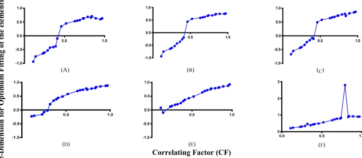
FIGURE 19. Experiments (A) to (C) shows the poor optimization for z with CF without using LT objects. However, we observe in (D) to (F) that model is learning to optimize itself for optimum CF for z-dimension using LT objects. The spike noticed in (F) is suspected to be error and will need future investigation. (A) through (C) were conducted using standard procedure where LT objects were not used.
FIGURE 20. The outcome shown here exhibits the model behavior for ratioRin terms of each dimension ofx,y and z. It is observed that
regression is relatively higher for each dimension and is considered pre-mature learning of the model.
and then 10 experiments were sampled to show the learning process of the model. As we observe (as expected) that the metrics are improved as we conducted more experiments. The experiment number indicates the sampling range of the total statistics.Errcorresponds to overall error for a single experiment once the learner process stabilizes anderr corre-sponds to local errorper experiment during a single training period. It is noted that Correlating Factor (CF) improves as the process learns with more experiments and data.
Fig 20 to 25provide the experimental outcomes of the vital functions such as Ratio (R), Adder, Remover, and various metrics to further validate the stability and optimum fitness of the proposed model. Some cases as shown also compare
FIGURE 21. The observation here shows improvement and considered mature classifier learning of theLTprocess. As we noticed that z-dimension (as hoped in the design of the model) is depreciating with respect of the error ratioR.
the ideal and real behavior of the model so it can be seen very clearly how close the model stays with the real-world test, specially when it is exhausted by the diverse set of data.
Table 5, 6 and 7 show the typical results of the3-D mea-sures. The snapshot of the results shows the difference of model behavior for theoretical (what we thought it will be) and experimental (what it turned out to be). These results are reported to support the model’s stability in real the world data in line with testing data.
Fig 19 shows six experimental studies of the proposed model. As discussed earlier, the model aims to achieve the fitness space optimization in z-dimension while it swings via its logical learning process between two extremes for underfit
FIGURE 22. Adder real and ideal function is shown here. We observe that when experiment size is at lower end, it shows higher % and as the experiment size increases, the function outcomes drop and this behavior is in line with model internals as expected. The triangular spike is a training error.
FIGURE 23. Remover real and ideal function is shown here. It shows that model exhibited theoretical stability of its internals.
FIGURE 24. This test shows the matching function built in eFES algorithm for random vs correlated data points. As we observed, it shows the promising behavior (expected) when it is highly correlated than just the random test without using LT objects.
and overfit (x,y). It must be noted, as we stated earlier that we are providing the sub-set of our diverse set of experiments for this article. We attempted to validate our model so that the
FIGURE 25. This test shows the candle stick analysis commonly used for stocks predictions. True Positive (TP), False Positive (FP), Fitness Factor (FF), Correlating Factor (FF), Bias Factor (BF) shows the move between 0 to 100 % for 20 experimental-run tests. This analysis helps particularly in understanding the direction of the move of the metric when classifier learns. For example, if we can consider the speed of the process, we can see the move in green candle from almost 0 to 98 % throughout the process.
reported simulations and experimental outcomes represent the model behavior, integrity, and stability in the real world.
VI. CLOSING REMARKS A. CONCLUSION
This article presented vital component as a Logical Table (LT) unit and its constructs in the internals of enhanced Machine Learning Engine Engineering (eMLEE) Model. LT worked at the lowest level of this engine and regulated the entire processing when model was blending and tuning various good fit algorithms. It enhanced the feature selection and opti-mization for optimum-fitting of the Machine Learning (ML) process for predictive analytics.LTconstructs introduced the novel parallelism for the enhanced algorithm blend classifier learning.LTconstructs provided a logical way of recording the metrics of the classifier learning for3Dobjects focused on overfit, underfit, and optimum fit for each algorithm’ and fea-ture’ incorporation during real time training. This approach uniquely supported the enhancement towards improved accu-racy, reduced errors, bias and overfitting.
Experimental datasets were split into test, train and valida-tion sets so the model learning and bias can be evaluated in a parallel fashion.
Overfitting, poor generalization, higher errors, low accu-racy, and bias became significant when blend was being engi-neered such aseMLEE. Thus,LTstructure was invented as a part ofeMLEEdevelopment to provide in-parallel regulation and governance of the metrics that needed to be recorded during the learning process. This approach also aided to the solution of addressing ‘No Free Lunch Theorem’ problem which generally does not ensure that a good fit algorithm is not left untested.