GPU-based Pedestrian Detection for
Autonomous Driving
Victor Campmany Canes
Abstract–Pedestrian detection has gained a lot of prominence during the last few years. Besides the fact that it is one of the hardest tasks within computer vision, it involves huge computational costs. Obtaining acceptable real-time performance, measured in frames per second (fps), for the most advanced algorithms is nowadays a hard challenge. In this work, we propose a GPU implementation of a well-known pedestrian detection system (i.e., HOGLBP-SVM) specially designed for the Tegra X1 embedded GPU. It includes LBP and HOG as feature descriptors and SVM as classifiers. We introduce significant algorithmic adjustments and optimizations to adapt the problem to the NVIDIA GPU architecture without sacrificing accuracy. The aim of this work is to offer a real-time system providing reliable results.
Keywords– Autonomous driving, pedestrian detection, computer vision, CUDA, massive paral-lelism
Resum– La detecci ´o de vianants ha estat un tema de molt inter `es els darrers anys. A part de ser una de les tasques m ´es complexes de la visi ´o per computador, implica uns costos com-putacionals molt elevats. Obtenir un rendiment de temps real acceptable, mesurat en imatges processades per segon (fps), per la majoria d’algoritmes m ´es avanc¸ats ´es una fita complicada. Aquest treball proposa una implementaci ´o en GPU d’un conegut detector de vianants (i.e., HOGLBP-SVM) dissenyat expressament per la Tegra X1, una GPU encastada. El detector inclou els m `etodes LBP i HOG com descriptors de caracter´ıstiques i un SVM com a classificador. El sistema introdueix ajustos algor´ıtmics i optimitzacions per adaptar el problema a l’arquitectura d’una GPU NVIDIA sense sacrificar precisi ´o. L’objectiu ´es proporcionar un sistema de temps real que alhora sigui robust. Paraules clau– Conducci ´o aut `onoma, detecci ´o de vianants, visi ´o per computador, CUDA, paral·lelisme massiu
F
1
I
NTRODUCTIONH
UMANfactor causes most of the driving accidents; consequently, autonomous driving is emerging as a solution. Autonomous driving will not only in-crease safety, but will also develop a system of a coopera-tive self-driving cars which will reduce pollution and con-gestion. Furthermore, it will enable handicapped people, elderly persons and kids to have more freedom.Autonomous driving requires perceiving and understand-ing the vehicle environment (e.g., road, traffic signs, pedes-trians, vehicles) using sensors (e.g., cameras, LIDAR’s, sonars, radar). It also requires a robust self-localization (using GPS, inertial sensors and visual localization in pre-cise maps), controlling the vehicle and planning the routes.
E-mail de contacte: [email protected] Menci´o realitzada: Enginyeria de Computadors Treball tutoritzat per: Dr. Juan Carlos Moure (CAOS)
These algorithms require high computation capability and real-time response.
Recently, with the appearance of embedded GPUs, au-tonomous driving is becoming attainable. Before its pres-ence, GPU-based autonomous driving applications were non-viable because of the high power consumption of GPUs and the need to be attached to a desktop computer. Nowa-days, the new NVIDIA’s Tegra X1 ARM processor repre-sents a promising approach. Tegra X1 is a low consumption processor designed for high demanding real-time applica-tions. Recently NVIDIA launched the Jetson TX1 and the DrivePX embedded platforms. Jetson TX1 equipped with one Tegra X1 processor is specially designed for robotics while NVIDIA Drive PX equipped with two TX1 proces-sors is specially designed for autonomous driving.
Accordingly, in this work we propose a pedestrian de-tector for the Tegra X1 ARM processor. The pedestrian detector is a key module for robotic applications and au-tonomous vehicles. It requires reliable algorithms and de-mands huge computational resources. Its aim is to
guish and locate humans on a digital image. Pedestrians present a wide variation in their poses, clothes, illumina-tions and backgrounds making pedestrian detection one of the hardest tasks of computer vision. Pedestrian detection has been an active research topic in the last twenty years. Several survey articles [1–3] show the advances achieved in this topic. One of the state of the art detectors is the Random forest of Local Experts [4]. However, the real-time con-straints in the field are tight, and recent works [4] proved that general purpose processors are not able to achieve real-time performance.
Any image-based pedestrian detector is composed by four core modules: the foreground segmentation, the fea-ture extraction, the classification and the refinement. The foreground segmentation generates candidate windows to contain pedestrians. These windows are described using distinctive patches in the feature extraction stage. Dur-ing the classification stage the windows are labeled usDur-ing a learnt model accordingly to its features. Finally, as a pedes-trian could be detected by several windows, these windows are merged in the refinement stage.
We propose to develop a real-time pedestrian detection system based on [4], specially designed for the Tegra TX1 processor. We have introduced significant optimizations to adapt the algorithm to the GPU architecture without sacri-ficing the detector accuracy. Our system is capable of run-ning in real-time in the DrivePX platform obtairun-ning state of the art accuracy.
The pedestrian detection application ported to the GPU is composed by different algorithms. Regarding the feature extraction process we distinguish two methods: Histograms of Local Binary Patterns (LBP) [5] and Histograms of Ori-ented Gradients (HOG) [6]. The foreground segmentation is done with the Sliding Window (SW) technique and the classification uses a Support Vector Machine (SVM) [7].
The rest of the paper is organized as follows. Section 2 introduces the state of the art; section 3 describes the baseline pedestrian detector while section 4 explains the methodology followed to achieve the objectives. In section 5 we analyze each algorithm and propose a mapping to the CUDA architecture and, section 6 provides the obtained re-sults. Finally, section 7 summarizes the work and section 8 outlines the future research lines.
2
S
TATE OF THE ARTGeneral Purpose GPU (GPGPU) computing consists on us-ing graphical processus-ing units to perform regular compu-tation. Traditionally, GPUs where designed to handle 3D graphics applications. However, the slow CPU improve-ments in terms of parallel processing incited the experts to exploit the outstanding capabilities of graphical processing units. Creating in this way the massively parallel computing paradigm that we know today.
Computer Unified Device Architecture (CUDA) is a plat-form created by NVIDIA to develop general purpose appli-cations for the GPUs [8]. NVIDIA’s GPUs are composed by tens of processing units calledStreaming Multiproces-sors(SMs). SMs share a L2 cache and an external Global Memory. Each SM has a Shared Memory that is managed explicitly and a L1 cache. A CUDAkernelis composed by thousands of threads executing the same program with
dif-ferent data. Threads are divided into groups of up to 1024 threads called Cooperative Thread Arrays (CTAs), which are atomically issued in one SM. The threads in a CTA col-laborate using the on-chip Shared Memory. Each CTA is divided into batches of 32 threads calledwarps. Threads within a warp can cooperate using a private set of registers. Finally, individual threads have a reserved memory region in each layer of the memory hierarchy called Local Mem-ory.
The warp is the minimum scheduling unit and it is exe-cuted in a SIMD fashion. If threads in the same warp need to follow different execution paths, each of the paths is ex-ecuted sequentially having some of the threads active and the remaining stalled; this circumstance is called divergence and it is a limitation that needs to be addressed when design-ing parallel algorithms.
A critical performance issue of the GPU is the memory access pattern of the algorithm. GPUs achieve full memory performance when the memory accesses arecoalesced. Co-alesced memory access refers to combining multiple mem-ory operations into a single memmem-ory transaction. To achieve coalescing, the 32 threads of the warp must access consecu-tive memory addresses. Data layout, memory transfers and work distribution become key factors in order to achieve the best performance when designing GPU algorithms.
Since the appearance of GPGPU, researchers have in-vested a lot of effort on porting their object detection al-gorithms to the GPU. Huge efforts have also been put on Field Programmable Gate Array (FPGA) designs, obtain-ing outstandobtain-ing results [9]. Nonetheless, the facilities that the CUDA environment offers in terms of code maintenance and reusability are more suitable for the constant chang-ing field of computer vision. Works such as [10] assert that exploiting the massively parallel paradigm for object detection algorithms outperforms a highly tuned CPU ver-sion [11]. Previously related researches like [12–14] de-veloped a GPU object detector using the well-known HOG-SVM approach obtaining a performance boost. However, in the previously cited works the evaluations are done on a desktop GPU, which is unfeasible for applications such as autonomous driving. In this work we propose a real-time pedestrian detector running on the NVIDIA DrivePX, a low consumption autonomous driving platform. Furthermore, as far as we know, the HOGLBP-SVM detection pipeline [15] has never been ported to the GPU.
3
P
EDESTRIAN DETECTIONWe will use Histograms of Local Binary Patterns (LBP) [5] and Histogram of Oriented Gradients (HOG) [6] for the fea-ture extraction. Both methods can be used individually with an SVM classifier, obtaining the LBP-SVM and HOG-SVM pipelines. As previous researches have shown [15] combin-ing both HOG and LBP by concatenatcombin-ing its feature vec-tors give better detection accuracy, creating the well-known HOGLBP-SVM pipeline.
LBP is a texture descriptor that, for each pixel in the input image, computes the output pixel depending on the values of the 8 nearest neighbor pixel values. Then, a histogram of these values is computed. The HOG method counts the occurrence of gradient orientation on a chunk of the im-age, understanding the gradient as the directional change of
color in an image.
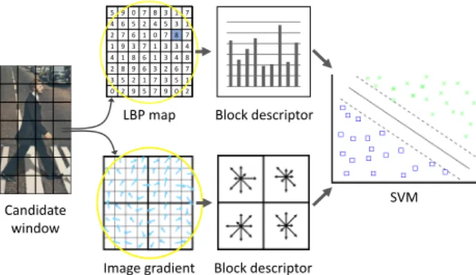
The Sliding Window (SW) algorithm is used as fore-ground segmentation method. It splits the image into rect-angular boxes, called windows, that are the candidates to contain pedestrians. Each window is classified with a Sup-port Vector Machine (SVM) [7]. The algorithm discrimi-nates the windows with pedestrians from the rest. SVM is a supervised learning model that builds a hyper-plane that is able to differentiate two categories (e.g. pedestrians from background). Figure 1 shows the feature description and classification of a candidate window using HOG, LBP and SVM.
In order to detect pedestrians of various sizes and at dif-ferent distances a image pyramid is generated. The im-age pyramid consists on the computation of multiple down-scaled copies of the input frame, called pyramid layers, each of them having different dimensions. Every layer is pro-cessed with the feature extraction and classification meth-ods, then the results of all the layers are refined using the non-maximum suppression algorithm [16].
SVM Candidate
window
Image gradient Block descriptor LBP map Block descriptor
5 9 0 7 8 3 1 7 4 6 5 2 4 5 3 1 2 7 6 1 0 7 8 7 1 9 3 7 1 3 3 4 4 1 8 6 1 3 4 8 2 8 9 6 3 2 6 7 3 5 2 1 7 3 5 1 0 2 9 5 7 9 0 2
Figure 1: HOGLBP-SVM candidate window classification. Each window of the sliding window is described with a fea-ture descriptor and then classified using a SVM.
4
M
ETHODOLOGYAn iterative process has been followed to achieve the objec-tive. We start by implementing a sequential version of each algorithm. The analysis of this implementation provides a better overview on the compute requirements, the data de-pendences and the parallelization options of the algorithm. With the acquired knowledge, a CUDA accelerated imple-mentation is developed. Once completed, the algorithm is evaluated using the available profiling tools in order to de-tect the performance bottlenecks. After profiling, an opti-mization evaluation is done with the collected data and the algorithm is tuned based on the profiler feedback.
5
D
EVELOPMENTWe have implemented three different detection pipelines sharing some of the basic algorithms mentioned in section 3 (i.e. LBP-SVM, HOG-SVM and HOGLBP-SVM). In this section we present the algorithms and discuss the de-cisions behind their massively-parallel implementations on a CUDA architecture. We start describing the general detec-tion pipelines and the design methodology, and then delve into the details of each algorithm.
5.1
Pipeline overview
The three detection pipelines considered in this work, or-dered from lower to higher accuracy and computational complexity, are LBP-SVM, HOG-SVM and HOGLBP-SVM. They represent three realistic options for an actual detection system, where one has to trade off functionality with processing rate. Figure 2 shows the pipeline stages: (1) the captured images are copied from the Host memory space to the Device; (2) the scaled-pyramid of images is created; (3) features are extracted from each pyramid layer; (4) every layer is segmented into windows to be classified; (5) detection results are copied to the CPU memory to exe-cute the Non-maximum Suppression algorithm that refines the results. Pipeline differences appear on the feature ex-traction stage. Image acquisition Pyramid Feature extraction Sliding Window & Classification Refinement
Host (CPU) Device (GPU)
Copy image to the GPU memory
Copy results to the CPU memory
Figure 2: Stages of the pedestrian detection pipeline on an heterogeneous computing system.
5.2
Local Binary Patterns (LBP)
Local Binary Patterns is a feature extraction method that gives information of the texture on a chunk of the image. The process can be divided into two steps: theLBP Map computation and theLBP Histogramscomputation.
The LBP Map [5] is computationally classified as a 2-dimensional Stencil pattern algorithm. The central pixel is compared with each of its nearest neighbors; if the value is lower than the center a 0 is stored, otherwise, a 1 is stored. Then, this binary code is converted to decimal to generate the output pixel value. Figure 3 illustrates the computation of a LBP Map value of a pixel.
(00001001) = 9 9 0 0 0 1 0 0 0 1 2 5 2 7 6 1 1 3 7
Figure 3: (1) Read central pixel; (2) Compare the central pixel with the 8 nearest neighbors and generate the binary code; (3) Convert the binary code to a decimal value; (4) Store the converted value into the output image.
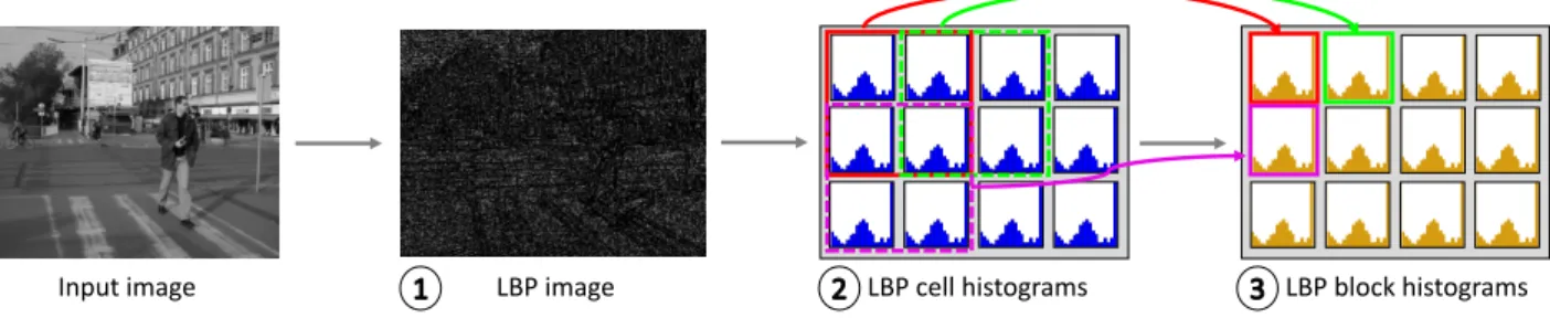
Finally, we extract the image features by computing the LBP Histograms. Histograms of blocks of16×16pixels are computed over the LBP image. The histograms have a50%overlap in theX andY axis meaning that each re-gion will be redundantly computed 4 times. We avoided the
Input image LBP image LBP cell histograms LBP block histograms
Figure 4: Steps to compute the LBP features of an image: (1) Given a grayscale image compute the LBP map (Algorithm 1); (2) compute the Cell Histograms of the LBP map (Algorithm 2); (3) histogram reduction to generate the Block Histograms (Algorithm 3).
redundant computing of the overlapped descriptors by split-ting theBlock Histogramsinto smallerCell Histogramsof 8×8pixels. Then, these partial histograms are reduced in groups of four (histogram reduction) to generate the output block histograms. Figure 4 shows the previously described sequence of operations to compute the LBP.
5.2.1 Analysis of parallelism & CUDA mapping for computing LBP
We implemented the 2-dimensional Stencil pattern by map-ping each thread to one output pixel (Algorithm 1). With this work distribution there are no data dependences among threads. Each thread performs 9reads(the central value and the eight neighbors) and 1storeand, the memory accesses are coalesced.
Algorithm 1: Massively parallel computation of the LBP map. FunctionLBPf performs the operations de-scribed in Figure 3.
input : I[H][W]
output: LBP[H][W]
1 parallelfory=0toH and x=0toWdo 2 LBP[y][x] =LBPf(y, x);
3 end
We designed two different solutions to compute the LBP histograms; the first one, is a straightforward paralleliza-tion without thread collaboraparalleliza-tion (Na¨ıve scheme); the sec-ond one, with thread collaboration, is designed to be more scalable (Scalable scheme).
The Na¨ıve scheme follows a Map pattern: each thread generates a Cell Histogram, avoiding the use of atomic op-erations. The histogram reduction is performed in the same way: each thread is mapped to a Block Histogram and the thread performs the histogram reduction.
The Scalable scheme solution aims for an efficient mem-ory access and data reutilization. Each thread is mapped to an input pixel of the image, and using atomic operations each thread adds to its corresponding Cell Histogram (Scat-ter pat(Scat-tern, see Algorithm 2). To generate the Block His-tograms every histogram reduction is performed by a warp (see Algorithm 3). With this design we attain coalesced memory access which leads to an scalable algorithm for dif-ferent image sizes. Our system uses the Scalable scheme as it attains better performance (see results in section 6.2).
Algorithm 2: Massively parallel computation of the Cell Histograms (Scalable scheme). Each thread reads a pixel and updates the corresponding cell. We use atomic operations (Read-Add-Store) to avoid data races. S ⇐histogram.
input : LBP[H][W]
output: CH[H/8][W/8][S]
1 parallelfory=0toH and x=0toWdo 2 bin = LBP[y][x];
3 atomicAdd(CH[y/8][x/8][bin], 1) ;
4 end
Algorithm 3: Massively parallel computation of the histogram reduction to generate the Block Histograms (Scalable scheme). FunctionhReductiongenerates the Block Histogram (Fa). Hb ⇐ H/8 − 1; W b ⇐
W/8−1.
input : CH[H/8][W/8][S]
output: Fa[Hb][Wb][S]
1 parallelfory=0toHb and x=0toWbdo 2 SIMD parallelforlane=0toWarpSizedo
3 t = lane; 4 whilet<Sdo 5 Fa[y][x][t] =hReduction(t); 6 t = t +WarpSize; 7 end 8 end 9 end
5.3
Histogram of Oriented Gradients (HOG)
The method of Histograms of Oriented Gradients [6] counts the occurrence of gradient orientation on a chunk of the image. The process could be divided into two steps: Gradientcomputation and theHistogramscomputation.
Gradient computation is used to measure the directional change of color in an image. The algorithm follows a 2 di-mensional Stencil pattern. The gradient of a pixel has two components, the magnitude (ω) and the orientation (θ). The orientation is the directional change of color and the mag-nitude gives us information of the intensity of the change. Figure 6 shows how the gradient of a pixel is obtained.
Histograms are computed by splitting the Gradient image into blocks of16×16pixels with50%overlap in X and Y
Input image Gradient magnitude (𝜔) ̶ Gradient orientation (𝜃) HOG block histograms
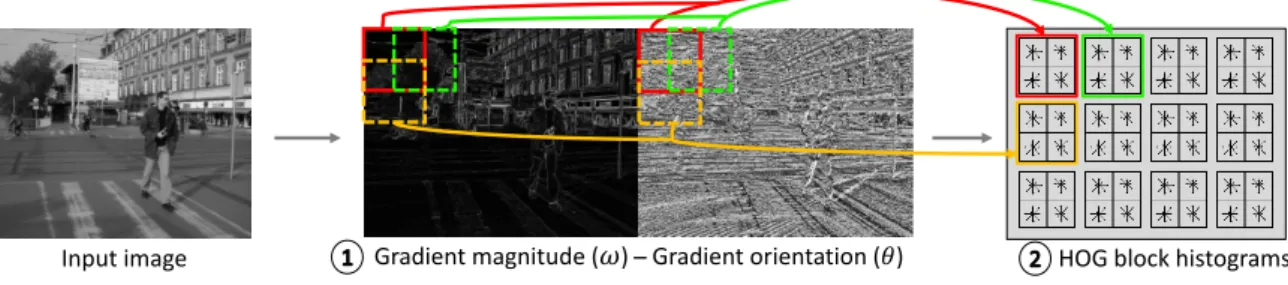
Figure 5: Steps to compute the HOG features: (1) given a grayscale image, compute the gradient (Algorithm 4); (2) compute the Block Histograms with trilinear interpolation (Algorithm 5).
𝑑𝑥 = 4 − 1 𝑑𝑦 = 7 − 3 𝜃 = 𝑎𝑟𝑐𝑡𝑎𝑛(𝑑𝑥, 𝑑𝑦) 𝜔 = 𝑑𝑥2+ 𝑑𝑦2 (𝜔, 𝜃) 7 4 6 1 3
Figure 6: (1) computedxanddywith the 4 nearest neighbor pixels; (2) computeωandθ; (3) storeωandθ.
axis (the same configuration as the LBP Histograms). In this case, because of histograms trilinear interpolation we can not compute8×8pixels Cell Histograms and then carry out the histogram reduction. Trilinear interpolation is used to avoid sudden changes in the Block Histograms vector (aliasing effect) [6]. Each Block Histogram is composed by four concatenated8×8pixels Cell Histograms. Different bins of the Block Histogram receive a weighted value of the orientation (θ) multiplied by the magnitude of the gradient (ω). Depending on the pixel coordinates, each input value could be binned into two, four or eight bins of the Block Histogram. The sequence of steps to compute the HOG features is described in Figure 5.
5.3.1 Analysis of parallelism & CUDA mapping for computing HOG
The gradient computation kernel follows a Map pattern: in-dividual threads are mapped to each output pixel (Algo-rithm 4). Single threads perform 4readsand 1store, and coalesced memory accesses are achieved.
Algorithm 4: Massively parallel computation of the Gradient. Each thread in the kernel performs the op-erations in Figure 6.
input : I[H][W]
output: M[H][W], O[H][W]
1 parallelfory=0toH and x=0toWdo
2 dx = I[y][x-1] - I[y][x+1]; 3 dy = I[y-1][x] - I[y+1][x]; 4 M[y][x] =sqrt(dx∗dx, dy∗dy); 5 O[y][x] =arctan(dx, dy);
6 end
The Histograms computation has been parallelized as-signing each thread to the computation of one histogram (Large-grain task parallelism, see Algorithm 5). With this structure there is no collaboration among threads and mem-ory accesses are not coalesced, though, the mapping avoids
the use of the costly atomic memory operations.
We implemented three different kernels following the scheme in Algorithm 5. The first one stores the data in Global Memory (HOG Global). To reduce the latency of the Global Memory we designed two more kernels: one stores the histograms in Local Memory, taking advantage of the L1 cache (HOG Local) and the other uses the on-chip Shared Memory (HOG Shared). In section 6.3 we will discuss the results of the implementations.
Algorithm 5: Massively parallel computation of the HOG Histograms. Fbis the vector of the HOG Block Histograms. Hb ⇐ H/8 −1; W b ⇐ W/8 −1;
S ⇐histogram
input : M[H][W], O[H][W]
output: Fb[Hb][Wb][S]
1 parallelfory=0toHb and x=0toWbdo 2 fori=0 to 16do
3 forj=0 to 16do
4 Fb[y][x]=updateBlockHistogram(i, j);
5 end
6 end
7 end
5.4
Sliding Window (SW) & Support Vector
Machine (SVM)
Sliding Window splits the image into highly overlapped re-gions of128×64pixels. Each window is described with a feature vector (~x). The vector is composed by the con-catenation of the Block Histograms (computed with HOG and LBP) enclosed in the given region. Then, every vector is evaluated to predict if the region contains a pedestrian or not.
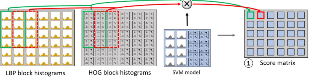
Support Vector Machine (SVM) is a supervised learning method that is able to discriminate two categories, in our case pedestrians from background [7]. After training the SVM, we obtain a model that performs as an n-dimensional plane that distinguishes pedestrians from background. The SVM training is done offline. However, the SVM infer-ence is done online. SVM gets as input a feature vector (~x) and computes its distance to the model hyper-plane (~ω). This distance is computed with the dot product operation. Then, the window is classified as pedestrian if the distance is greater than a given threshold and as background other-wise. Figure 7 shows the steps needed to evaluate each
win-LBP block histograms
Score matrix
SVM model
HOG block histograms
Figure 7: Sliding Window and SVM inference of the HOG and LBP features: (1) each window is evaluated computing the distance of the HOG and LBP features from the SVM model (Algorithm 6).
dow taking HOG and LBP features as the image descriptors.
5.4.1 Analysis of parallelism & CUDA mapping for SW-SVM
We first implemented a na¨ıve version (Na¨ıve SVM) with a Large-grain task parallelism and no thread collaboration. Each thread is responsible of the computation of the dot product between the candidate window (~x) and the model (~ω). The approach was not scalable and became critical as it is the kernel with the largest workload of the pipeline (see results on section 6.4).
To efficiently compute the dot product we designed a CUDA kernel where each warp is assigned to a window (~x) of the transformed image (Warp-level SVM). The compu-tation of the dot product is divided between the threads in the warp. Once intra-warp threads have computed the par-tial results, these are communicated among threads using register shuffle instructions and then reduced. Algorithm 6 shows the mapping of the Sliding Window and SVM infer-ence to the massive parallel architecture.
We decided to use a warp-level approach to avoid the overhead of thread synchronization as warps have implicit hardware synchronization. This configuration allows the full utilization of the memory bandwidth as the memory ac-cesses are coalesced.
6
E
XPERIMENTS& R
ESULTSIn this section we present the obtained performance results. We carry out the performance evaluation of individual al-gorithms and the application pipeline. All the experiments are ran with an Intel i7-5930K processor, a NVIDIA GTX 960 and a NVIDIA Tegra X1 as the target processor. First, we present the whole pipeline results and following we will discuss the results of individual methods. We will measure the efficiency of each of the algorithms with the follow-ing performance metric: processed pixels per nanosecond (px/ns); we will also refer to it asPerformance.
The pipeline experiments in section 6.1 are done using 12 pyramid layers. The performance evaluation in the re-maining subsections is done with a single pyramid layers as it is focused on the individual algorithms.
We should not directly compare the performance of the GTX 960 and the Tegra X1. A desktop GPU is designed to be reliable for graphical based application and the power consumption is not the main priority. The Tegra X1 em-bedded system, though, is intended to operate in
con-Algorithm 6: Massively parallel computation of the Sliding Window and the SVM inference.Nis the SVM trained model,HnandWnare the number of Block His-tograms fitting in a window andSis the histogram size. Hb⇐H/8−1;W b⇐W/8−1.
input : Fa[Hb][Wb][S], Fb[Hb][Wb][S] N[Hn][Wn][S]
output: scores[Y][X]
1 parallelfory=0toY and x=0toXdo 2 SIMD parallelforlane=0 to WarpSizedo
3 t = lane;
4 fori=0toHmdo
5 forj=0toWmdo
6 whilet<Sdo
7 res += Fa[i+y][j+x][t]∗N[i][j][t];
8 res += Fb[i+y][j+x][t]∗N[i][j][t];
9 t = t +WarpSize;
10 end
11 end
12 end
13 res =SIMDreductionSum(res);
14 iflane== 0then
15 scores[y][x] = res;
16 end
17 end
18 end
strained environments and power consumption is a con-cern. To compare both systems we introduce a new metric: P erf ormance/W att. To assess the Watt consumption we use the Thermal Design Power (TDP).TDPis the amount of heat generated by the processor in typical use cases; the attribute is provided by the manufacturer company.
6.1
Pipeline overview
In this section we evaluate the overall results of the sys-tem in terms of processing performance and the accuracy of the methods. To evaluate the application we use the KITTI dataset [17]. First we analyze the processing performance and then we detail the accuracy of the system.
To evaluate theP erf ormancewe use a video sequence with an image size of1242×375pixels. Table 1 presents the performance results of the LBP-SVM, HOG-SVM and HOGLBP-SVM pipelines, measured in processed frames per second (FPS). Results show the achieved FPS for the
multithreaded CPU baseline application [4] and the GPU accelerated version, for both desktop GPU and Tegra X1. Results prove that we have accomplished the objective of running the application in real-time under the low consump-tion ARM platform.
Pipeline LBP HOG HOGLBP
CPU 4 3.2 2.5
GTX 960 263 175 119
Tegra X1 40 27 20
Table 1: Performance of the detection pipelines measured in processed frames per second (FPS) in the different archi-tectures.
Figure 8 illustrates the miss rate depending on the false positive per image (FPPI). FPPI is the number of candidate windows wrongly classified as pedestrians, it can be under-stood as the tolerance of the system. As the FPPI increases, the miss rate decreases leading to a more tolerant system.
Figure 8: The numbers on the legend are the area bellow the curve (the lower the better). It is the objective term to be minimized in order to attain a reliable detector.
The system is able to achieve state of the art accuracy with the HOGLBP-SVM detection pipeline. The remain-ing pipelines (LBP-SVM and HOG-SVM) have slightly lower accuracy; nonetheless, they demand less computa-tional power to achieve real-time performance which make them suitable for less powerful GPUs.
6.2
Local Binary Patterns (LBP)
This section analyzes the two schemes developed to carry out the LBP computation. Figure 9 shows the obtained re-sults for different image sizes. The performance is mea-sured inpx/ns(the higher the better).
The experiments done with the profiling tools confirm that the memory operations are the bottleneck of the process both on the CPU and the GPU. As the workload becomes bigger, the Na¨ıve scheme suffers a decrease of performance caused by the poor memory management. However, the Scalable scheme performance remains constant for the exe-cuted experiments.
Obviously, running the kernels on the Tegra X1 pro-cessor has a decrease of performance, even though, if we
0 0,5 1 1,5 2 2,5 320x240 960x480 1280x853 2272x1704 Per for mance Image size
CPU GPU - Naïve GPU - Scalable Tegra X1 - Naïve Tegra X1 - Scalable
Figure 9: Performanceof the LBP feature extraction pro-cess (LBP map+LBP Histograms).
take into account theP erf ormance/W attmetric we con-clude that the X1 processor achieve a higher performance ratio for the executed experiments. Table 2 exposes the at-tainedP erf ormance/W attfor the Scalable scheme. The Tegra’s performance by power unit is 2.4 times higher than the GTX 960’s one.
GPU P erf ormance/W att
GTX 960 - Scalable 0,02
Tegra X1 - Scalable 0,048
Table 2:P erf ormance/W attof the extraction of the LBP features (LBP map+LBP Histograms).
6.3
Histograms
of
Oriented
Gradients
(HOG)
In this section we present the results of the HOG computa-tion for the CPU version and the GPU implementacomputa-tions. Ev-ery GPU kernel suffers a problem of non coalesced memory access, so the memory hierarchy is not efficiently managed. Additionally the parallelism is low, and the GPU compute resources are not fully exploited.
The Local Memory kernel takes advantage of the L1 cache to store the histograms. However, the threads running in a Streaming Multiprocessor (SM) have a working set big-ger than the size of L1 cache, leading to a high miss rate. To prove the fact and find out the suitable number of threads per SM we carried out various experiments restricting the number of resident threads per Multiprocessor (see Figure 10). As a consequence of the limitation of threads per SM, the working set is smaller and the data could fit into the L1 cache. Figure 10 shows the relation between the number of resident threads per SM and the performance measured in processed pixels per nanosecond. Empirically we can con-firm that the best performance is at 256 threads per SM. The remaining experiments for the HOG Local kernel are done using the optimal number of threads (256 threads per SM).
The HOG Shared kernel takes advantage of the fast on-chip Shared Memory. In this case the working set per thread is the same as the one described for the HOG Local ker-nel. However, in this case we do not have L1 cache miss problems as Shared Memory is explicitly managed by the programmer. Despite a GPU utilization of 25% because of
Shared Memory limitations, we obtain a significant increase of performance compared to the HOG Local kernel.
0 200 400 600 800 1000 0 0,05 0,1 0,15 0,2 0,25
Active threads per SM
Perf
or
m
an
ce
Figure 10: Performanceof the HOG Local kernel for dif-ferent number of threads per SM on the GTX 960.
Figure 11 shows the performance measured in number of pixels processed per nanosecond for the CPU code and the three CUDA kernels. The Shared Memory version out-stands all the previously implemented solutions, obtaining a 4x speedup compared to the Local Memory version.
0 0,1 0,2 0,3 0,4 0,5 0,6 0,7 0,8 0,9 1 320x240 960x480 1280x853 2272x1704 Pe rf or manc e Image size
CPU GPU - HOG Global GPU - HOG Local GPU - HOG Shared Tegra X1 - HOG Global Tegra X1 - HOG Local Tegra X1 - HOG Shared
Figure 11:Performanceof the HOG feature extraction pro-cess (Gradient computation+HOG Histograms).
The results prove that the first parallel version was not competitive even with a CPU code. For all the experiments, the CPU version performs similarly compared to the HOG Local kernel executed on the Tegra X1. However, the HOG Local kernel performance in the GTX 960 is slightly better than in the CPU. This fact determine that the limitations in terms of memory bandwidth of the Tegra system require a greater effort to gain significant speed-ups with respect to a CPU implementation.
Regarding the Shared Memory kernel, we increase the performance more than 2 times on both devices compared to the HOG Local kernel. Table 3 presents the accomplished P erf ormance/W attof the Shared Memory design. De-spite being almost 3 times slower, the Tegra X1 perfor-mance by power unit doubles theP erf ormance/W attof the GTX 960.
GPU P erf ormance/W att
GTX 960 – Shared Mem. 0,0061
Tegra X1 – Shared Mem. 0,0129
Table 3: AchievedP erf ormance/W attof the HOG fea-tures computation (Gradient computation + HOG His-tograms).
6.4
Sliding Window (SW) & Support Vector
Machine (SVM)
The classification via Sliding Window is the most time con-suming part: it takes up to55%of the time to process an image. For this reason, we have put a lot of effort to de-velop an efficient CUDA version and the results have been satisfactory.
The Warp-level kernel achieves almost full GPU occu-pancy, and peak memory performance. Figure 12 shows the performance of the two kernels (Na¨ıve kernel and Warp-level kernel) and the CPU implementation measured in number of pixels processed per nanosecond. Achieving ef-ficient coalesced memory access allowed us to attain 10x speed-up relative to the Na¨ıve kernel on the GTX 960. The Tegra X1 Warp-level kernel also takes advantage of the memory coalescing and obtains an 8x increase of perfor-mance. However, the Warp-level scheme suffers a decrease of performance as the image becomes bigger. When the image does not fit in the L2 cache the miss rate increases and data needs to be fetched and retrieved from the slower Global Memory. 0 0,1 0,2 0,3 0,4 0,5 0,6 0,7 320x240 960x480 1280x853 2272x1704 Per for m ance Image size
CPU GPU - Naïve GPU - Warp-level Tegra X1 - Naïve Tegra X1 - Warp-level
Figure 12: Performance of the Sliding Window +SVM candidate window evaluation.
Table 4 shows theP erf ormance/W attfor the Warp-level scheme. The Tegra performance by power unit is again higher, in this case almost double.
GPU P erf ormance/W att
GTX 960 – Warp-level 0,005
Tegra X1 – Warp-level 0,009
Table 4: AchievedP erf ormance/W attof the the Sliding Window+SVM candidate window evaluation.
7
C
ONCLUSIONSIn this work we show a massively parallel implementation of a pedestrian detector that uses LBP and HOG as features and SVM for classification. Our implementation is able to achieve the real-time requirements on the autonomous driv-ing platform, the NVIDIA DrivePX.
Our experiments confirm the importance of adapting the problem to the GPU architecture. Smart work dis-tribution and thread collaboration are key factors to at-tain significant speed-ups compared to a high end CPU.
The stated facts become even more critical when the de-velopment is done under a low consumption platform like the Tegra X1 processor. For the developed algorithms the P erf ormance/W att of the Tegra X1 doubles the GTX 960 one. The evidence determines that the Tegra ARM platform is an energy efficient system able to challenge the desktop GPU performance when running massively parallel applications.
With the methodology followed, we could compare the performance of different massively parallel mappings for a given algorithm and find out its drawbacks. We consider that this methodology has been successful to understand the organization and behavior of the CUDA architecture.
8
F
UTURE WORKThis work opens the gate to promising possibilities in the real-time autonomous driving applications. The developed system could be generalized to multi-class detection in or-der to recognize other objects appearing in a driving scene such as cars, motorcycles or traffic signs.
The next step is to improve the accuracy of the system with a Random Forest classifier. Additionally the pedestrian detector is ready to be integrated with a 3D-vision system to improve the perception of the scene.
ACKNOWLEDGMENTS
I would like to thank Dr. Juan Carlos Moure for his uncon-ditional help and patience, without him this project would not be possible. Moreover, I would like to thank Dr. Anto-nio M. L´opez and Dr. David V´azquez for their confidence on me and for letting me be part in this promising project at the Computer Vision Center. Finally, I would like to ac-knowledge the work done by Sergio Silva, who gave me constant support with the GPU software and hardware.
Our research is also kindly supported by NVIDIA Corpo-ration in the form of different GPU hardware and technical support.
R
EFERENCES[1] D. Geronimo, A. M. Lopez, A. D. Sappa, and T. Graf. Survey of pedestrian detection for advanced driver as-sistance systems. InPAMI, 2010.
[2] D. M. Gavrila. The visual analysis of human move-ment: A survey. InCVIU, 1999.
[3] P. Dollar, C. Wojek, B. Schiele, and P. Perona. Pedes-trian detection: An evaluation of the state of the art. In PAMI, 2012.
[4] J. Marın, D. V´azquez, A. M. L´opez, J. Amores, and B. Leibe. Random forests of local experts for pedes-trian detection. InICCV, 2013.
[5] T. Ojala, M. Pietikainen, and T. Maenpaa. Multireso-lution gray-scale and rotation invariant texture classi-fication with local binary patterns. InPAMI, 2002. [6] N. Dalal and B. Triggs. Histograms of oriented
gradi-ents for human detection. InCVPR, 2005.
[7] C. Cortes and V. Vapnik. Support-vector networks. In Machine learning, 1995.
[8] E. Lindholm, J. Nickolls, S. Oberman, and J. Mon-trym. Nvidia tesla: A unified graphics and computing architecture. InIEEE micro, 2008.
[9] M. Hahnle, F. Saxen, M. Hisung, U. Brunsmann, and K. Doll. Fpga-based reat-time pedestrian detection on high-resolution images. InCVPR, 2013.
[10] R. Benenson, M. Mathias, R. Timofte, and L. Van Gool. Pedestrian detection at 100 frames per second. InCVPR, 2012.
[11] P. Dollar, S. Belongie, and P. Perona. The fastest pedestrian detector in the west. InBMVC, 2010. [12] C. Wojek, G. Dork´o, A. Schulz, and B. Schiele.
Sliding-windows for rapid object class localization: A parallel technique. InPattern Recognition, 2008. [13] L. Zhang and R. Nevatia. Efficient scan-window based
object detection using gpgpu. InCVPR, 2008. [14] V. A. Prisacariu and I. Reid. fasthog - a real-time gpu
implementation of hog. InTechnical Report, 2009. [15] X. Wang, T. X. Han, and S. Yan. An hog-lbp human
detector with partial occlusion handling. In ICCV, 2009.
[16] I. Laptev. Improving object detection with boosted histograms. InImage and Vision Computing, 2009. [17] A. Geiger, P. Lenz, C. Stiller, and R. Urtasun. Vision