General Type-2 Radial Basis Function Neural Network: A Data-Driven Fuzzy Model

Citation for published version:

Rubio-Solis, A, Melin, P, Martinez-Hernandez, U & Panoutsos, G 2019, 'General Type-2 Radial Basis Function Neural Network: A Data-Driven Fuzzy Model', IEEE Transactions on Fuzzy Systems, vol. 27, no. 2, 8417444, pp. 333-347. https://doi.org/10.1109/TFUZZ.2018.2858740 DOI: 10.1109/TFUZZ.2018.2858740 Publication date: 2019 Document Version Peer reviewed version

Link to publication

(C) 2018 IEEE. Personal use of this material is permitted. Permission from IEEE must be obtained for all other uses including reprinting/republishing this material for advertising or promotional purposes, creating new collective works for re-sale or re-distribution to servers or lists, or reuse of any copyrighted components of this work in other works.

University of Bath

General rights

Copyright and moral rights for the publications made accessible in the public portal are retained by the authors and/or other copyright owners and it is a condition of accessing publications that users recognise and abide by the legal requirements associated with these rights. Take down policy

If you believe that this document breaches copyright please contact us providing details, and we will remove access to the work immediately and investigate your claim.

General Type-2 Radial Basis Function Neural

Network: A Data-Driven Fuzzy Model

Adrian Rubio-Solis

, Patricia Melin

, Uriel Martinez-Hernandez

and George Panoutsos

Abstract—This paper proposes a new General Type-2 Radial Basis Function Neural Network (GT2-RBFNN) that is function-ally equivalent to a GT2 Fuzzy Logic System (FLS) of either Takagi-Sugeno-Kang (TSK) or Mamdani type. The neural struc-ture of the GT2-RBFNN is based on theα-planes representation, in which the antecedent and consequent part of each fuzzy rule uses GT2 Fuzzy Sets (FSs). To reduce the iterative nature of the Karnik-Mendel algorithm, the Enhaned-Karnik-Mendel (EKM) type-reduction and three popular direct-defuzzification methods, namely the 1) Nie-Tan approach (NT), the 2) Wu-Mendel uncer-tain bounds method (WU) and the 3) Biglarbegian-Melek-Mendel algorithm (BMM) are employed. For that reason, this paper provides four different neural structures of the GT2-RBFNN and their structural and parametric optimisation. Such optimisation is a two-stage methodology that first implements an Iterative Information Granulation approach to estimate the antecedent parameters of each fuzzy rule. Secondly, each consequent part and the fuzzy rule base of the GT2-RBFNN is trained and optimised using an Adaptive Gradient Descent method (AGD) respectively. Several benchmark data sets, including a problem of identification of a nonlinear system and a chaotic time series are considered. The reported comparative analysis of experimental results is used to evaluate the performance of the suggested GT2 RBFNN with respect to other popular methodologies.

Index Terms—General Type-2 FLSs, Radial Basis Function Neural Networks, α-plane representation, fuzzy modelling.

I. INTRODUCTION

G

and is gaining more and more in popularity [1]–[6]. This is mainly credited to the capability of General Type-2 Fuzzy Sets (GT2 FSs) to better handle and minimise the effect of high levels of uncertainty with respect to other high order FSs such as Interval Type-2 Fuzzy Sets (IT2 FSs) [7]–[14]. Compared to Type-1 Fuzzy Sets (T1 FSs) and IT2 FSs, a GT2 FS weights uncertainty nonuniformly and is described by a Memberhip Function (MF) that is characterised by more parameters, so using GT2 FSs allows for more design degrees of freedom [7], [14]. Furthermore, a GT2 FS is characterised by a Footprint of Uncertainty (FOU) and an MF (secondary MF), where uncertainty can be modelled with any degree between 0 and 1, whereas T1 and IT2 FSs associate uncertainty only to crisp values of 0 or 1 respectively [9].

1 _{A. Rubio-Solis and G. Panoutsos are with the department of Automatic}

Control and Systems (ACSE), The University of Sheffield, Sheffield, S1 3JD

UK.a.rubiosolis, [email protected]

2 _{Patricia Melin is with the Division of Graduate Studies Tijuana Institute}

of Technology Tijuana, [email protected]

3 _{Uriel Martinez-Hernandez is with the Department of Electronic and}

Electrical Engineering, Faculty of Engineering and Design, University of Bath,

Bath, BA2 7AY, [email protected]

TABLE I:ABBREVIATIONS AND THEIR DEFINITIONS.

Abbreviation Definition

A2-C0 Antecedents are type-2 fuzzy sets and_{Consequents are type-0 fuzzy sets (crisp)}

AED Average of End-points Defuzzification

AGD Adaptive Gradient Descent

BMM Biglarbegian Melek Mendel approach

COS Center Of Sets (type-reduction)

EKM Enhanced Karnik-Mendel algorithm

FOU Foot Print of Uncertainty

GT2 FS General Type-2 Fuzzy Set

IIG Iterative Information Granulation

IWA Interval Weighted Average

LMF Lower Membership Function

MF Membership Function

NT Nie-Tan simplification.

RBFNN Radial Basis Function Neural Network

T1 FLS Type-1 Fuzzy Logic System

T2 FLS Type-2 Fuzzy Logic System

TR Type Reduction.

TSK Takagi Sugeno Kang

UMF Upper Membership Function

WM UBs Wu Mendel Uncertainty Bounds

As indicated in [7], a GT2 FLS can be thought as a high order fuzzy set uncertainty model with more flexibility. Therefore, a GT2 Fuzzy Logic System has the potential to outperform not only the use of FLSs of T1, but also to provide a performance than an FLS with IT2 FSs cannot achieve [7]. Although GT2 FLSs are still in their infancy, the number of aplications of higher order fuzzy systems has experienced an important increase during the past five years [15], in particular in areas such as Pattern Recognition [12], [13], Automatic Control [2], [16], Image Processing [17] and Robotics [1], [3], [18]. In this applied context, the usage of GT2 FSs usually increases the computational complexity with respect to T1 and IT2 FLSs. This is clearly compensated not only by a higher model accuracy but also with a better treatment of uncertainty that can be obtained by using GT2 FSs as well as due to new computing technologies. For example in [19], a Mamdani fuzzy neural network with a hidden layer that employs GT2 FSs was proposed. In [19], a comparison about the prediction of noisy time series between the proposed GT2 neural network (NN), a monolithic network and an IT2 NN revealed the superiority of GT2 models to better manage uncertainty. In [17], the authors developed an edge detection system based on a morphological gradient technique and GT2 FSs.

Fuzzifier Inference engine Rules Type-Reducer Defuzzifier GT2 Fuzzy Input Sets Measured crisp inputs Crisp Outputs Type-reduced set Output Processing GT2 Fuzzy Output Sets y = f(x )p

GT2 Fuzzy Logic System

T1 Fuzzy set

y ϵ Y

x ϵ X

Fig. 1:General Type-2 Fuzzy Logic System (GT2 FLS, Taken from [9]).

According to [17], the proposed GT2 edge detection ar-chitecture showed a higher performance than IT2 and T1 FLSs for edge detection when image processing is under high levels of noise. Similar to T1 and IT2 FLSs, a GT2 FLS involves a similar architecture as illustrated in Fig. 1. Specifically, an FLS can be regarded of GT2 if only one of the associated FSs is of GT2 [7]. In this sense, several efforts have been made to represent GT2 FLSs (or T2 FLSs) [20]– [22]. Particularly, horizontal slice-representation allows using everything learned in IT2 FSs theory [9]. According to the

α₋cut decomposition theorem, α₋cuts decomposition offers

a practical way to represent GT2 FLSs (including of IT2 and T1). This is because a GT2 FLS can be represented as the

union of all its α−planes raised to a level α, where each

α−plane is the union of itsα−cuts [9]. Thus, based on the

α−cuts decomposition theorem, at each inputx0_{=~xp, a GT2}

FLS simultaneously uses α−cuts for each vertical slice over

the secondary MF domain and the associated α₋planes [9].

Based on the α₋plane representation, in this paper a new

General Type-2 Radial Basis Function Neural Network (GT2-RBFNN) that is functionally equivalent to a GT2 Mamdani (or TSK) FLS is suggested. To provide a high trade-off between accuracy and model simplicity, two different GT2 RBFNN structures are implemented. On the one hand, to reduce the iterative nature of the Karnik-Mendel method (KM), a GT2 RBFNN with an Enhanced KM algorithm is suggested. On the other hand, three different GT2 RBFNN structures based on direct-defuzzification methods are also presented, i.e. a GT2 RBFNN with a a) Nie-Tan approach, a b) Wu-Mendel Uncertainty bounds method and a c) Biglarbegian-Melek-Mendel procedure. A learning methodology based on an Iterative Information Granulation process (IIG) and an Adaptive Gradient Descent (AGD) approach is implemented to identify the parameters of each antecedent and consequent in the rule base of a GT2 RBFNN. The major contributions of the GT2 RBFNN are twofold. The first contribution is the proposal of a novel RBFNN based on GT2 FSs. Current applications only focus on novel learning methodologies and the implementation of metaheuristics to improve the generali-sation properties of the RBFNN. The suggested GT2 RBFNN incorporates GT2 FSs not only to better model and minise the effects of uncertainty, but also to provide a higher level of model accuracy than its counterparts the RBFNN and

the IT2 RBFNN. Compared to ensemble of neural networks where uncertainty is viewed as a measure of disagreement among on some inputs, a GT2 RBFNN treats uncertainty as a deficiency that results not only from imprecise boundaries in the FSs of an RBFN and IT2 RBFNN, but also as consequence of information-based imprecision. The second contribution is the proposal of GT2 RBFNN structures based on direct-defuzzification methods and the implementation of an adaptive learning for model simplification and improvement of the convergence of a traditional gradient descent approach.

The rest of this paper is organised as follows: In Sections II and III, a brief review of T2 FSs and the functional equivalence between the RBFNN and GT2 FLSs is provided. Sections IV and V detail the architecture of a GT2-RBFNN with an EKM and three simplified neural structures respectively. In Section V, a parameter identification approach for the GT2 RBFNN models is described. A comparative analysis and a discussion of experiments results are presented in Sections VI and VII correspondingly. Finally, conclusions are drawn in section IX.

II. GENERALTYPE-2 FUZZYLOGIC

This section provides a brief review of General Type-2

Fuzzy Sets (GT2 FSs) and theory ofα-plane representation.

A. Definition of a General Type-2 Fuzzy Set

A General Type-2 Fuzzy Set (GT2 FS) denoted byA˜(also

called T2 FS) is characterised by a bivariate MFµA˜(x, u)⊆

[0,1] on the Cartesian product µA˜ : X ×[0,1], where the

primary variable is x _∈ X. And the y ₋ axis is called

secondary variable or primary MF u _∈ Jx ⊆ [0,1] as

illustrated in Fig. 2. Thus,A˜is represented by:

˜

A=_{(x, u), µ_A˜(x, u)|∀x∈X,∀u∈Jx⊆[0,1]} (1)

{µ_A˜(u)|u∈U} is a vertical slice ofµ_A˜(x, u)and it can also

be represented by itsα₋cut decomposition.

B. α₋plane Representation

Anα₋plane for a GT2 FSA˜is denoted byA˜α, is the union

of the primary MFs ofA˜whose secondary grades are greater

than or equal toα(0_≤α_≤1)

˜

Aα={(x, u), µA˜(x, u)≥α|x∈X, u∈[0,1]} (2)

where the lower and upper limits forA˜α are defined by

(

LM F( ˜Aα) =aα˜

U M F( ˜Aα) =bα˜

(3)

That means whenA˜αis raised to levelα, it is a plane at that

level that can be obtained by connecting all the corresponding

α₋cutsof the associated vertical slices of the secondary MFs

of x_∈X [7]. Hence, the horizontal-slice representation of a

GT2 FSA˜ is defined by ˜ A= sup α∈[0,1] α/ Z x∈X [aα(x), bα(x)]/x = [ α∈[0,1] α/A˜α (4)

x u µ_A˜(x, u) α-plane 1/A˜1 1 3/A˜13 ˜ A0 1.0 1.0 1.0

Fig. 2:Someα−planes raised to levelαfor a GT2 FS (Taken from [7]).

III. RADIALBASISFUNCTIONNEURALNETWORK AND

GENERALTYPE-2 FUZZYLOGICSYSTEMS

It has been proven that under some mild conditions the RBFNN can be viewed as a Type-1 Fuzzy Logic System of either Mamdani or Takagi-Sugeno-Kang type (TSK) [23], [24]. This equivalence has been further extended in [24] in order to design an Interval Type-2 RBFNN (IT2 RBFNN) with a Karnik-Mendel type-reduction in which all the fuzzy sets are of Interval Type-2. An RBFNN can be regarded as an FLSs whose main inference engine is interpreted as an adaptive filter [7], [24]–[26]. It resembles an additive weighted combination of the MFs of the fired-rule output sets in the hidden layer of the RBFNN (See Fig. 3) [7]. Thereby, every hidden receptive unit in the RBFNN is functionally equivalent

to a fuzzy rule Ri _{described by a multi-variable Gaussian}

MFµRi(~x_p, y_p) =µ_Ri[x₁, . . . , x_n, y], where the input vector

~xp∈X1×. . . Xn and the implication engine is defined as:

µRi(~x_p, y) =µ_Ai_→Gi = h Tkn1µFki(xk)? µG i_(y) i (5)

Where?is the minimumt₋normthat represents the shortest

Euclidean distance to the input vector~xp. And each receptive

unit is the ithfuzzy rule:

Ri:IF x1 isF1i and. . .IF xk isFki and. . .

IF xn isFni THENy isGi; i= 1, . . . , M (6)

So that, the firing strengthfi of each receptive unit is

µAi_→Gi(~x_p, y) = n Y k=1 µFi k(xk) =fi exp " − Pn k=1(xk−mki)2 σ2 i #! (7)

where Ai = F1i ×. . .×Fni - mki and σi are the center

and width of a multi-variable Gaussian MF respectively. By

combining all the rules in the output layer, yp is [27]

yp= PM i=1µAi_→Gi(~x_p, y)w_i PM i=1µAi_→Gi(~x_p, y) (8) x₁ x₂ x₃ x_k x_n w₁ y_p w₂ w₃ w_i f(·)_M w_M f(·) i f(·)₃ f(·)₂ f(·)₁

Input layer Hidden layer Output layer

Fig. 3:Radial Basis Function Neural Network (RBFNN, Taken from [23]).

Strictly speaking, any kind of FLS enhancement might be directly applicable to the RBFNN theory because the structure of its fuzzy rule base in going from T1 FSs to T2 FSs does not change; it is the way the associated antecedents and consequents are modelled [7]. Thus, an RBFNN can be functionally equivalent to a kind of GT2 FLS that is based on the horizontal-slice representation if an RBFNN consists of:

I. An input layer with a singleton fuzzification.

II. The T-norm operator used to compute each rule’s firing strength is multiplication (meet).

III. The secondary MF of each GT2 FS is convex.

IV. Theα₋cut of each T1 secondary MFA,˜ A˜αis given by

a set of the lower and upper firing strengths

fα i, fαi

as described in Fig. 4.

The structure of an RBFNN can be viewed as GT2

Takagi-Sugeno-Kang FLS if for eachithfuzzy rule

˜

Ri

α:IF x1 isF˜1i and. . .IF xk isF˜ki and. . .

IFxn isF˜ni THENy is˜gi(~xp); i= 1, . . . , M (9) whereas for a Mamdani inference fuzzy system, the

conse-quent part is defined as ’y is G˜i_{’. For a GT2 RBFNN of}

Mamdani (TSK) type, when ~xp = x0l, a vertical slice in the

ith receptive unit for theith antecedentF˜i

k is activated, and

itsα₋cut decomposition is given by:

˜ Fki(x0l)⇔µ_A˜i_→G˜i(~xp, y) = sup α∈[0,1] α/ fαi, fαi (10)

For simplicity, it is used fα

i(~xp) = fαi. Hence, the level α

firing set in each receptive unit is defined by

Fα i ≡ fα i, fαi , α_∈[0,1] (11) Built upon a horizontal-slice representation, a GT2 RBFNN can be defined as [28]

1. A horizontal-slice Mamdani (TSK) FLS that is analogous to an IT2 FLS where a number of operations described for IT2 FSs theory occur for each horizontal slice [7]. 2. A Wagner-Hagras (WH) GT2 RBFNN FLS that results

from the union over αof the horizontal-slice Mamdani

~xp u µ_A˜p i(~xp, u) Vertical Slice 1.0 0.75 0.5 0.25 α/fαi(~xp) LMF α/fαi(~xp) α/fαi(~xp) UMF x0 l • • • •

Fig. 4: Singleton fuzzification and triangle secondary MF that is activated when~xp=x0_lfor theithreceptive unit of the RBFNN

IV. GENERALTYPE-2 RADIALBASISFUNCTIONNEURAL

NETWORK(GT2 RBFNN)

Based on Fig. 5, this section describes the GT2 RBFNN structure that can be viewed as a Mamdani (TSK) GT2 FLS with an Enhanced Karnik-Mendel (EKM) type-reduction layer, where all the FSs are of GT2. For demonstration purposes,

here a GT2 RBFNN with an uncertain width σi = [σi1, σ2i]

and a fixed mean mi

k is implemented. A horizontal-slice

representation is used for the simplest Mamdani (TSK) GT2 RBFNN structure that consists of a singleton fuzzification with a secondary MF that is convex, a Center-Of-Sets (COS) type reduction that uses an EKM and an average of end-points defuzzification (AED) as described in Fig. 6. To avoid additional parameters, and as shown in 4, the secondary MFs are vertical slices, a triangle function is employed where its

base is equal to f0

i −f0i and its Apex location given by

Apex(~xp) =f0i(~xp) + 1 2w[f 0 i(~xp)−f0i(~xp)];w∈[0,1] (12) A. GT2RBFNN Input Layer

The proposed GT2 RBFNN is a Multi-Input-Single-Output FLS, in which the input data is a multidimensional crisp vector

represented by~xp= [x1, . . . , xn]∈Rnwhere only the current

state is fed into the layer and then forwarded to next layer.

B. General Type-2 RBF Layer

It is assumed a singleton fuzzification, i.e. for each value

xk only a T1 vertical slice for an antecedent GT2 FS F˜ki

is activated. Compared to an IT2 RBFNN, to describe each horizontal slice in the GT2 layer of a GT2 RBFNN, a number

of Sfiring strengths[fαs

i , fαis]is required (See Fig. 6) where

α2> α1. At input~xp, for each fuzzy rule in the GT2-Mamdani

(TSK) RBFNN, only one firing interval Fαs

i is activated for

level αsin the GT2 RBF layer as (See Fig. 6, 7 and 8) [29]:

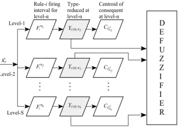
Rule-i firing interval for level-α Type-reduced at level-α Centroid of consequent at level-α Fα₁ i Fα2 i FαS i

D

E

F

U

Z

Z

I

F

I

E

R

Fig. 5:GT2 Mamdani computations for an RBFNNN (Taken from [7]).

Fαs i :=                  Fαs i = [f αs i (~xp), fαis(~xp)] fαs i (~xp) =exp " − n X k=1 xk−mik σ2 i 2# αs fαs i (~xp) =exp " − n X k=1 _x k−mik σ1 i 2# αs (13)

Note the termαis not a variable [7]. The subscript0s0 _{is used}

to denote eachα-level in the GT2 RBFNN.

C. Type-reduction Layer

In the type reduction layer, a Center Of Sets Type Reduction (COS TR) is used. This layer performs a mathematical oper-ation that maps a GT2 FS into a T1 FS. Hence, the centroid

of each consequent at theαs-plane is computed as:

CG˜i αs =αs/[w i l,αs, w i r,αs] (14)

According to [7], [29], for a Mamdani GT2 RBFNN, [wi

l,αs, w

i

r,αs] is an Interval Weighted Average (IWA) that is

used along with the firing intervalFαs

i to compute the reduced

set[yαs

l (~xp), yrαs(~xp)]for αs-level as:

yαs l = PLαs i=1 wil,αsf αs i + PM i=Lαs+1w i l,αsf αs i PLαs i=1fαis+ PM i=Lαs+1f αs i (15) yαs r = PRαs i=1 wr,αi sf αs i + PM i=Rαs+1w i r,αsf αs i PRαs i=1 fαis+ PM i=Rαs+1f αs i (16) where YCOS,αs = 1/[y αs l (~xp), yαrs(~xp)]. For a TSK GT2

RBFNN, a normalised A2−C0 GT2 FLS version is used

in which the antecedents are GT2 FSs, and the associated

consequent isgi,αs=c

i,αs

0 x0+ci,α1 sx1+. . .+ci,αn sxn, where

x0= 1 andci,αms,(m= 0, . . . , n)are crips numbers.

yαs l = PLα i=1gi,αsf α i +P M i=Lα+1gi,αsf α i PL i=1fαi + PM i=Lα+1fαi (17) yαs r = PRα i=1gi,αsf α i + PM i=Rα+1gi,αsf α i PRα i=1fαi + PM i=Rα+1fαi (18)

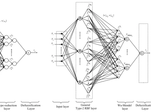
x1 x₂ x₃ x_k x N y L y_R y_p General Type-2 RBF layer

Input vector layer

Type-reduction layer y L y R f₁α 1 f 1 α1 f₁α s f 1 αs α1 α1 αS αS [w , w li r i ] , αs , αs Input layer Σ Defuzzification Layer f₂α 1 f₂α S f_iα 1 f_iα S f M α1 f_MαS f_Mα1 f_Mαs f_iα s f_iα 1 f₂α s f₂α 1

Fig. 6:GT2 RBFNN with an EKM type-reduction layer.

D. Defuzzification Layer

This layer performs defuzzification that consists of a process of aggregation of all horizontal slices. Here, the Average of End-Points Defuzzification (AEPD) is used [14]:

yp(~xp) = S X s=1 αs[(yαls(~xp) +yrαs(~xp))/2] , _S X s=1 αs (19)

V. SIMPLIFIEDGENERALTYPE-2 RADIALBASIS

FUNCTIONNEURALNETWORK

In this paper, a GT2 RBFNN that employs a direct-defuzzification algorithm as an output layer is called Simpli-fied General Type-2 Radial Basis Function Neural Network (SGT2 RBFNN). For practical reasons, particularly for real world T2 FLSs, the need to bypass the iterative nature of KM algorithms that results from the number of permutations that are needed to calculate the reduced set has become a priority. Type-reduction is usually used as going from a T2 FS to a T1 FS [30]. In this paper, the term direct-defuzzification and closed-form type reduction are used indistinctly to refer to the mapping that goes from a GT2 FS to a crisp number (type-0). Due to their simplicity and accuracy with respect to KM algorithms, in this paper three popular direct-defuzzification approaches [30] are selected, i.e. a) Nie-Tan closed-form (NT) [31], b) Wu-Mendel Uncertain Bounds approach (WU) [32] and c) the Biglarbegian-Melek-Mendel method (BMM) [33].

A. Simplified Wu-Mendel GT2-RBFNN

The second simplified structure is a Mamdani GT2-RBFNN that employs the Wu-Mendel Uncertain Bounds method and

that is called WM GT2-RBFNN for short. For eachα-level in

the GT2-RBFNN, the WM method replaces the type reduction x1 X 2 x₃ x_k x_N y p General

Type-2 RBF layer Wu-Mendel layer

f 1 α1 f₁α s f₁α _s f_iα 1 f_Mα1 f_iα 1 f_Mα1 f_iα s f_Mαs f M αs [w , w li r i ] , α_s , α_s Input layer Σ Defuzzification Layer α_S y_r y_rα S y lα 1 y l α1 Σ Σ y l α S y l α_S α1 y r y_rα 1 y _α 1 WM, y _α S WM, f 1 α1 f_iα S Fig. 7:Wu-Mendel GT2 RBFNN.

with an approach that calculates the inner and outer-bound sets for the type reduced of IT2 FLSs [32]. As shown in Fig. 7,

for each input vector~xp, the WM GT2RBFNN output is

yp(~xp) = S X s=1 αsyW M,αs , _S X s=1 αs (20)

For eachα₋level,yW M,αs is computed as:

yW M,αs = 1 4 y αs l (~xp) +yαls(~xp) +yrαs(~xp) +yαrs(~xp) (21) where yαs l =y αs l −       Fp× M X i=1 fαs i w i l,αs−w 1 l,αs M X i=1 fαs i w M l,αs−w i l,αs M X i=1 fαs i wl,αi s−w 1 l,αs + M X i=1 fαs i wMl,αs−w i l,αs       (22) yαs r =yαrs+       Fp× M X i=1 fαs i wr,αi s−w 1 r,αs M X i=1 fαs i wMr,αs−w i r,αs M X i=1 fαs i wr,αi s−w 1 r,αs + M X i=1 fαs i wMr,αs−w i r,αs       (23)

x₁ x₂ x 3 x_k x_N y_p General Type-2 RBF layer

Input vector layer

f₁α s

f M

α1

w_i αs

Input layer Nie-Tan

Layer Σ Σ Σ y NT,α₁ y NT,α_S f_MαS f_iα 1 f_iα S f 1 α1 f₁α S f₁α 1 f_iα 1 f_iα s f_Mα1 f_MαS Fig. 8:Nie-Tan GT2 RBFNN. Where Fp = PM_i=1 fαis−f αs i /PM i=1f αs i PM i=1f αs i . in

which, consequents wi,αs are different for eachα−level. The

terms yαs

l andyαrs are given by

yαs l =min (_M X i=1 fαs i w i l,αs/ M X i=1 fαs i , M X i=1 fαs i w i l,αs/ M X i=1 fαs i ) (24) yαs r =max (M X i=1 fαs i wir,αs/ M X i=1 fαs i , M X i=1 fαs i wir,αs/ M X i=1 fαs i ) (25) B. Simplified Nie-Tan GT2-RBFNN

The second structure is a GT2-RBFNN that uses the Nie-Tan method as a direct-defuzzification layer as illustrated in Fig. 8. The Nie-Tan is a direct-defuzzification method initially developed for IT2 FLSs. Such method uses the vertical repre-sentation of the Footprint of Uncertainty (FOU) [31] before the process of dedifuzzification to finally compute the centroid of the IT2 FS. The NT layer can be considered a zero order Tay-lor series approximation of Karnik-Mendel+dedifuzzification methods. It has been proved the Nie-Tan operator is equivalent to an exhaustive and accurate type-reduction for both discrete and continuous IT2 FSs [31]. Although there has been im-provements on the Nie-Tan operator, in this paper, the centroid

yN T,αs at each α−level is calculated as:

yN T,αs = PM i=1w αs i f αs i +f αs i PM i=1f αs i + PM i=1f αs i (26)

For each input vector ~xp, the NT GT2RBFNN output yp(~xp)

is calculated as: yp(~xp) = S X s=1 αsyN T,αs , S X s=1 αs (27) x1 x₂ x₃ x_k x_N y_p General

Type-2 RBF layer BMM layer

f₁α 1 f₁α _s f_iα 1 f_Mα1 f₁αs g _i,αs Input layer Σ Defuzzification Layer y _α 1 BMM, f_iαs f_Mαs y _α S BMM, f₁α 1 f_iα S f iα 1 f_Mα1 f_MαS Fig. 9:Biglarbegian-Melek-Mendel GT2 RBFNN. C. Simplified Biglarbegian-Melek-Mendel GT2-RBFNN

As an alternative to computing the output of a TSK GT2-RBFNN is the Biglarbegian-Melek-Mendel closed form equa-tion [33]. The last simplified neural structure that is called

TSK BMM GT2-RBFNN for short. According to Fig. 9ypis:

yp(~xp) = S X s=1 αsyBM M,αs , S X s=1 αs (28)

for eachαs-plane:

yBM M,αs=mαsy αs m +nαsy αs n (29) In which yαs m = PM i=1gi,αsf αs i / PM i=1f αs i and yαns = PM i=1gi,αsf αs i / PM i=1f αs i . The terms f αs i and f αs i are

cal-culated using (13), and consequents gi,αs and adaptation

parametersmαs andnαsare different for eachα−level, where

gi,αs=c

i,αs

0 x0+. . . ci,αmsxm forx0= 1.

VI. LEARNINGMETHODOLOGY OF THEGT2 RBFNN

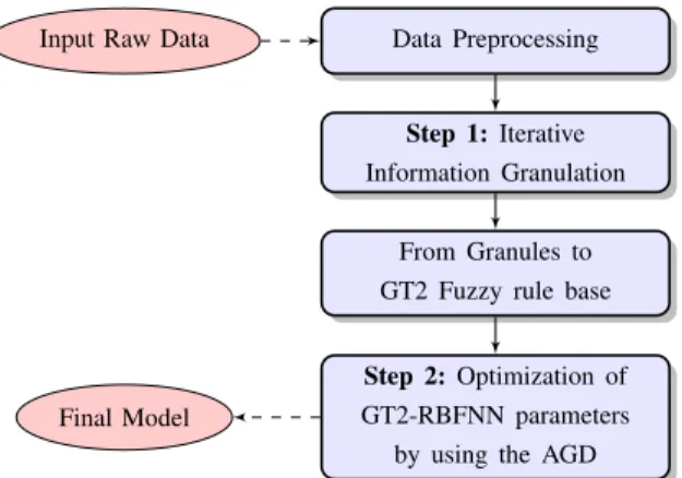
To identify the optimal parameters of the GT2 RBFNN, and its neural structure, a two-stage learning methodology based on the concept of Iterative Information Granulation (IIG) and an Adaptive Gradient Descent (AGD) approach is implemented. IIG is a clustering technique whose main essence is to discover a structure in data while producing representatives called granules [34]. Such granules are formed based on a data compatibility measure, and their geometrical properties are used to estimate the initial values of each antecedent in the GT2 RBFNN (See flow diagram, Fig. 10). Similarly to [26], the number of fuzzy rules or hidden units in the GT2 RBFNN is initially approximated by using the gradient of the compatibility curve that is obtained by the IIG.

Data Preprocessing Input Raw Data

Step 1:Iterative Information Granulation

From Granules to GT2 Fuzzy rule base

Step 2:Optimization of GT2-RBFNN parameters

by using the AGD Final Model

Fig. 10:Parameter identification applied to the GT2 RBFNN.

In a second stage, AGD is applied to optimise the parameters

σ1

i, σ2i

, and mi

k and to determine the optimal number of

fuzzy rules according to cross-validation results.

A. Iterative Information Granulation

In this work, IIG is used not only to granulate/cluster data (Fig. 11), but also used as an approximation to the optimal number of fuzzy rules (hidden nodes) in the GT2 RBFNN as

well as the initial values for[σ1

i, σ2i]andmik of each MF [26].

The process of IIG is based on a compatibility indexC(A, B)

that defines how good is the merging operation of any two

granulesAandB. IIG consists of two main steps: [34], [35]:

• Find the two most ’compatible’ information granules A

and B by using Eq. (30) and merge them together as a

new information granulegi= (lki, uki)[26]. Wheregiis

defined by its lower and upper corners (lik, uik) for the

dimension 0k0 andi= 1, . . . , M.

• Repeat the process of finding the two most compatible

granules until a satisfactory data abstraction level is achieved. Where the compatibility ’C’ is defined as [34]:

C(A, B) =DM AX−dA,B·e

−αgcardA,B /CardinalityMAX_{LA,B /LengthMAX}

(30)

Such asDM AX,LengthM AX and the termCardinalityM AX

is the maximum possible distance and length of a granule and the total number of granules in the data set respectively.

dA,Bis the weighted multidimensional average distance of the

resulting granule with wk playing the importance weight for

the dimension k. In Eq. (30), αg weights the requirements

between distance and cardinality/length and LAB is the

mul-tidimensional length of the resulting granulegi, where:

dA,B= 1 n n X k=1 wk(max(uAk, uBk)−min(lAk, lBk)) (31)

giis used as a fuzzy constraint to extract the initial parameters

of LMF and UMF (mk andσi) which are calculated as:

mik = 1 2(lik−uik) ; m i k = [mi1, ..., min]; i= 1, . . . , M (32) x1 x2 x3 1 2 3 4 5 6 7 8 9 10 11 12 13 14 15 16 17 18 19 20 1 ₂ 3 4 5 6 7 8 9 10 11 1 2 3 4 5 maxx 1− minx 2 Granule A Granule B Granule C

Fig. 11:3-D Example of final Data space for a set of granules A, B and C.

(σ1 i)2= 1 r   r X j=1 kmj_k−mi kk   1/2 j₆=i; σ2 i =σi1−∆σi (33)

in whichj6=i, andj is the nearest neighbour to theithfuzzy

rule, andr≥2 [36].

B. Adaptive Gradient Descent Approach (AGD)

After structure identification, the common parameters mi

k and[σ1

i, σ2i]of the antecedent GT2 MFs as well as the

weight-ing factors[wil,αs, w

i

r,αs]at eachα−level of a Mamdani (TSK)

GT2 RBFNN should be optimised. Here, an Adaptive Gradient Descent (AGD) approach that evaluates the Root-Mean-Square

Error (RMSE) and uses a performance indexPi= _P1PPp=1e2p

is applied [37]. For eachpinput-output training data(~xp, dp);

p = 1, . . . , P, a cost function Ep = 1₂(e2p) is also defined,

where the error ep = (yp(~xp)−dp), and dp is the desired

pattern. To increase the convergence performance of a typical Gradient Descent approach and avoid getting trapped in a local

minimum, a momentum term γ is introduced. A self-tuning

learning rateβis defined to enhance the learning performance

of the GT2-RBFNN. As feedback information, at each current

and previous learning iteration ’t’, the change trend ofPi is

evaluated and used to adjust the value ofγandβ as follows:

• ifP i(t+ 1) ≥ Pi(t)Then β(t+ 1) =hdα(t), γ(t+ 1) = 0 • ifP i(t+ 1) < Pi(t)and ∆P i P i(t) < δ Then β(t+ 1) =hiα(t), γ(t+ 1) =γ0 (34) • ifP i(t+ 1) < Pi(t)and ∆P i Pi(t) ≥δThen β(t+ 1) =β(t), γ(t+ 1) =γ(t)

where hd,(0< hd <1) andhi,(1< hi) are the decreasing

and increasing factors respectively andδis a threshold rate for

the RMSE. Thus, by using an EKM type reduction, at each

α₋level of a GT2 RBFNN, the AGD must be able to track the

corresponding parameters σi andmik in the antecedent active

branch in which the value of Lα and Rα may change [24].

As pointed out in section III, a GT2 RBFNN is analogous to an IT2 FLS where all the IT2 FS computations occur for each horizontal slice and their aggregation is carried out by a

defuzzification process [7]. Hence, for eachα−level, the final

AGD equations for the consequents[wl,α, wr,α]of a Mamdani

GT2-RBFNN are updated as: ∆wil,αs(p+ 1) =−β ∂Ep(~xp) ∂wi l,αs +γ∆wl,αi s(p) (35) ∆wir,αs(p+ 1) =−β ∂Ep(~xp) ∂wi r,αs +γ∆wir,αs(p) (36)

For a TSK GT2-RBFNN, the consequent coefficientsci,αs

m are updated according to ∆ci,αs m (p+ 1) =−β ∂Ep(~xp) ∂ci,αs m +γ∆ci,αs m (p) (37)

To update the common parameters mi

k and σ1 i, σ2i ∆mik(p+ 1) =−β ∂Ep(~xp) ∂mi k +γ∆mik(p) (38) ∆σi1(p+ 1) =−β ∂Ep(~xp) ∂σ1 i +γ∆σi1(p) (39) ∆σi2(p+ 1) =−β ∂Ep(~xp) ∂σ2 i +γ∆σi2(p) (40)

Therefore, the derivatives ∂Ep(~xp)/∂mik, ∂Ep(~xp)/∂σi1 and

∂Ep(~xp)/∂σi2 should equal the addition of their updates for

each α−level as follows

∂Ep ∂mi k = S X s=1 ∂Ep ∂mi k αs (41) where ∂Ep ∂mi k|αs

is the partial derivative ofEp with respect to

the parameter mi k at thesth α−level. ∂Ep ∂mi k αs = 2dαep _∂yαs l ∂fαs i +∂y αs r ∂fαs i _∂fαs i ∂mi k + _∂yαs l ∂fαs i +∂y αs r ∂fαs i _∂fαs i ∂mi k (42) Where ∂Ep(~xp)/∂yp(~xp) =αs2PS_s=1αs, and the derivative

∂yp(~xp)/∂y_lαs =∂yp(~xp)/∂yrαs.dα=αs/4PS_s=1αsis used

to simplify notation. To update σ1

i andσi2 ∂Ep ∂σ1 i = S X s=1 ∂Ep ∂σ1 i αs ; ∂Ep ∂σ2 i = S X s=1 ∂Ep ∂σ2 i αs (43) where ∂Ep ∂σ1 i _α s = 2dαep ∂yαs l ∂fαs i +∂y αs r ∂fαs i ∂fαs i ∂σ1 i (44) ∂Ep ∂σ2 i αs = 2dαep _∂yαs l ∂fαs i + ∂y αs r ∂fαs i _∂fαs i ∂σ2 i (45)

where the derivatives∂fαs

i /∂σi2and∂f αs

i /σ1i are zero. At

each α₋plane, the AGD approach tracks each permutation

that results for the implementation of an EKM method in order to calculate the derivatives with respect to each weight

∂Ep(~xp)/∂wil,αs and ∂Ep(~xp)/∂w

i

r,αs and the coefficients

ci,αs

m of a GT2 RBFNN of Mamdani and TSK type

respec-tively. In [24-26], a detailed description of this calculation for an IT2 fuzzy NN and an IT2 RBFNN with a Mamdani inference and using a KM method is provided.

C. AGD for simplified GT2-RBFNN

Compared to a GT2-RBFNN that utilises an EKM algo-rithm, direct-defuzzification-based structures do not need a sorting process. Thereby, the implementation of the AGD to identify the parameters of a GT2-RBFNN of Mamdani (TSK) type results much simpler.

1) Wu-Mendel GT2-RBFNN: To update the parameters of

a WM GT2RBFNN of Mamdani type, the derivatives with

respect to the weighting factorswi

l,αs andw i r,αs, and common parametersσ1 i,σi2, andmik are: ∂Ep ∂wi l,αs =dαep ∂yW M,αs ∂wi l,αs ; ∂Ep ∂wi r,αs =dαep ∂yW M,αs ∂wi r,αs (46) ∂Ep ∂mi k = S X s=1 ∂Ep ∂mi k αs (47) so that: ∂Ep ∂mi k αs =dαep _∂yαs l ∂fαs i + ∂y αs l ∂fαs i +∂y αs r ∂fαs i +∂y αs r ∂fαs i _∂fαs i ∂mi k (48) wheredα=αs/4PS_s=1αs, and to update [σi1, σ2i]

∂Ep ∂σ1 i = S X s=1 ∂Ep ∂σ1 i αs ; ∂Ep ∂σ2 i = S X s=1 ∂Ep ∂σ2 i αs (49) so that ∂Ep ∂σ1 i αs =dαep _∂yαs l ∂fαs i +∂y αs l ∂fαs i +∂y αs r ∂fαs i + ∂y αs r ∂fαs i _∂fαs i ∂σ1 i (50) ∂Ep ∂σ2 i αs =dαep _∂yαs l ∂fαs i +∂y αs l ∂fαs i +∂y αs r ∂fαs i + ∂y αs r ∂fαs i _∂fαs i ∂σ2 i (51)

Where the term∂yl/∂wl,αi s and∂yl/∂w

i l,αs is ∂yl ∂wi l,αs =            fi/ M X i=1 fi, min n y_l(0), y(_lM)o=y_l(0) fi/ M X i=1 fi, min n y_l(0), y(_lM)o=y_l(M) (52)

∂yαs l ∂wi l,αs = ∂y αs l ∂wi l,αs −(Fp)        fαs i M X i=1 fαs i wMl,αs−w i l,αs − fαs i M X i=1 fαs i wil,αs−w 1 l,αs M X i=1 fαs i w i l,αs−w 1 l,αs + M X i=1 fαs i w M l,αs−w i l,αs !2        (53)

A similar procedure is used to calculate the terms ∂yαs

r /∂wir,αs and ∂y

αs

r /∂wr,αi s. To exemplify the computation of the

derivatives∂fαs

i /∂mik,∂f αs

i /∂mik, ∂yαrs/∂fαis,∂yαrs/∂fiαs,∂yαrs/∂fαis and∂yαrs/∂fαis, the calculation of∂y αs l /∂f αs i and ∂yαs l /∂f αs i is shown below: ∂yαs l ∂fαs i =                    wr,αi s M X i=1 fαs i M X i=1 fαs i ! − M X i=1 fαs i −f αs i M X i=1 fαs i ! M X i=1 fαs i M X i=1 fαs i !2 , min n y(0),αs r , y(rM),αs o =y(0),αs r 0, minny(0),αs r , yr(M),αs o =y(M),αs r (54) ∂yαs l ∂fαs i = y αs l ∂fαs i +               −vq M X i=1 fαs i M X i=1 fαs i ! − M X i=1 fαs i −f αs i M X i=1 fαs i M X i=1 fαs i M X i=1 fαs i !2        +vr(wil,αs−w 1 l,αs)       M X i=1 fαs i −f αs i M X i=1 fαs i M X i=1 fαs i              (55)

in which, the termsvq andvr are:

vq =       M X i=1 fαs i wil,αs−w 1 l,αs M X i=1 fαs i wl,αMs−w i l,αs M X i=1 fαs i w i l,αs−w 1 l,αs + M X i=1 fαs i w M l,αs−w i l,αs       vr=        vl M X i=1 fαs i wl,αMs−w i l,αs − M X i=1 fαs i wil,αs−w 1 l,αs M X i=1 fαs i wMl,αs−w i l,αs ! M X i=1 fαs i w i l,αs−w 1 l,αs + M X i=1 fαs i w M l,αs−w i l,αs !2       

In which vl is used to simplify notation as vl=PMi=1f

αs i wi l,αs−w 1 l,αs +PM i=1fi wM l,αs−w i l,αs .

2) Nie-Tan GT2-RBFNN: For a NT GT2-RBFNN of

Mam-dani type, the AGD equations are defined for the consequent

weight of each α₋level as an spikewαs

i and updated as:

∆wαs i (p+ 1) =−β ∂Ep(~xp) ∂wαs i +γ∆wαs i (p) (56) To implement the AGD for a Mamdani NT GT2-RBFNN, the

derivative ∂Ep(~xp)/∂wαis in (56) is updated as

∂Ep(~xp) ∂wαs i = ∂Ep(~xp) ∂yN T,αs(~xp) ∂yN T,αs(~xp) ∂wαs i (57) where:∂Ep(~xp)/∂yN T,αs(~xp) =αs/

PS s=1αs and ∂yN T,αs ∂wαs i = f αs i +fαis PM i=1f αs i + PM i=1f αs i (58) Consequently,σ1

i,σi2 andmik are adjusted as

∂Ep(~xp) ∂σ1 i = ∂Ep(~xp) ∂yN T,αs _∂y N T,αs ∂fαs i ∂fαs i ∂σ1 i (59) ∂Ep(~xp) ∂σ2 = ∂Ep(~xp) ∂yN T,αs _∂y N T,αs ∂fαs i ∂fαs i ∂σ2 i (60) where ∂yN T,αs ∂fαs i =∂yN T,αs ∂fαs i = w αs i −yN T,αs PM i=1f αs i + PM i=1f αs i (61) in which ∂fαs i ∂σ1 i = 2fαs i (xk−mik)2 (σ2 i)3 ; ∂f αs i ∂σ2 i = 2fαs i (xk−mik)2 (σ2 i)3 (62) ∂fαs i ∂mi k = 2fαs i (xk−mik) (σ2 i)2 ; ∂f αs i ∂mi k = 2fαs i (xk−mik) (σ1 i)2 (63)

For a TSK GT2-RBFNN, the AGD approach follows a similar procedure described in Eq. (59-63). However, the consequent coefficientsci,αs

m for eachα−level are updated as:

∂Ep(~xp) ∂ci,αs m =∂Ep(~x)p ∂yN T,αs xm(fαis+fαis) PM i=1f αs i + PM i=1f αs i ! (64)

wherem= 0, . . . , n, such thatx0= 0andci,αms= 1.

3) Biglarbegian-Melek-Mendel GT2-RBFNN: Based on the

AGD approach, in order to update the parameters of a TSK

BMM GT2-RBFNN with an uncertain [σ1

i, σ2i], fixed mean

mi

k and consequentsgi,αs for eachα−level

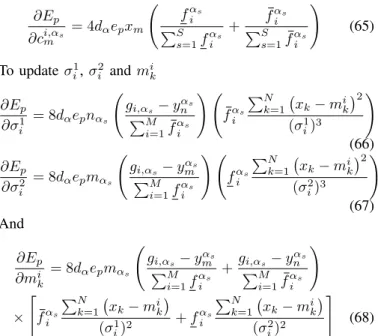
∂Ep ∂ci,αs m = 4dαepxm fαs i PS s=1f αs i + f αs i PS s=1f αs i ! (65) To update σ1 i,σi2 andmik ∂Ep ∂σ1 i = 8dαepnαs gi,αs−y αs n PM i=1f αs i ! fαs i PN k=1 xk−mik 2 (σ1 i)3 ! (66) ∂Ep ∂σ2 i = 8dαepmαs gi,αs−y αs m PM i=1f αs i ! fαs i PN k=1 xk−mik 2 (σ2 i)3 ! (67) And ∂Ep ∂mi k = 8dαepmαs gi,αs−y αs m PM i=1f αs i +gi,αs−y αs n PM i=1f αs i ! × " fαs i PN k=1 xk−mik (σ1 i)2 +fαs i PN k=1 xk−mik (σ2 i)2 # (68)

Please note for each α−level, a different value for the

coeff-cients ci,αs

m is employed.

VII. PERFORMANCEVERIFICATION

In this section, three different examples are used to compare the performance of the GT2 RBFNN structures with some well known algorithms such as the ANFIS, a Sequential Adaptive Fuzzy Inference System (SAFIS) [38], a network of Functionally Weighted Single-Input-Rule-Modules connected to a Fuzzy Inference System (FWSIRM-FIS) [38], Support Vector Regression (SVR), RBFNN of T1 and IT2, an ensemble of T1 RBFNNs based on a Negative Correlation Learning (E-RBFNN) [39], Support Vector Machine (SVM) [40], Least Square SVM (LS-SVM) [40] and an IT2 Fuzzy Neural Net-work with support vector regression (IT2-FNN-SVR) [41]. While the first example involves the modelling of 10 real-world benchmark data sets for multiclass classification and regression problems, the last two examples are used for nonlin-ear plant identification and chaotic time series prediction in the precense of randomness and Gaussian noise respectively. For the ANFIS, RBFNN, IT2-RBFNN and GT2 RBFNN models and E-RBFNN, all the simulations are carried out in MATLAB 2014 environment in an intel Core i7, 2.7 GHZ CPU. Similar to a GT2 RBFNN, an AGD version is implemented to train the RBFNN and the IT2 RBFNN [24], [42].

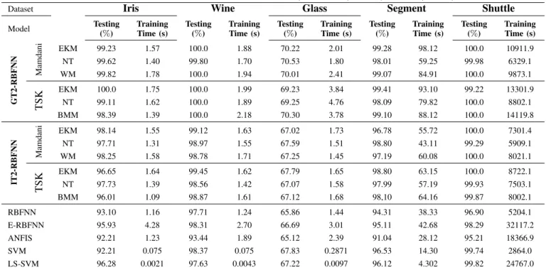
A. Example 1: Modelling of Benchmarck Data sets for Mul-ticlass Classification and Regression

This example compares the performance of a GT2 RBFNN, RBFNN, IT2 RBFNN, E-RBFNN, ANFIS, SVM and LS-SVM on five real-world benchmark data sets for regression and five data sets for multiclass classification. In Table II and III, the specifications of the data sets are listed. The associated distributions of the data sets are unknown and most of them noisy-free. As indicated in Tables II and III, for cross-validation purposes the number of samples for training (column train) and testing (column test) are randomly selected. By increasing/decreasing by one the number of hidden units initially estimated by the IIG algorithm, the optimal number of hidden units (fuzzy rules) in the GT2 RBFNN are selected

based on cross-validation results. In Tables II-III, columnfuzzy

rulesis used to indicate the optimal value for the number of

hidden units for the RBFNN, IT2 RBFNN and GT2 RBFNN

models. It is selected a granulation factor of αg = 0.3, an

initial value for ∆σi = 0.1, σ1i = 1.0 and for wl,αi s = 1.0

and wi

r,αs = 1.0. For a TSK GT2 RBFNN with a BMM

method, it was determined that the best value for mα = 0.9

and nα = 0.1. For all GT2 RBFNN models and for the

E-RBFNN, it was found the best trade-off between accuracy and model simplicity is achieved by using three horizontal slices and 4 units in the hidden layer. In Tables IV and V, the generalisation performance of SVM, and LS-SVM presented in [41] is compared to the average performance results of 20 trials for the ANFIS, RBFNN, IT2 RBFNN, E-RBFNN and GT2 E-RBFNN. As indicated in [40], SVM and LS-SVM usually achieves a good generalisation performance. This heavily depends on the combination of values for the

cost parameterC and kernel parameterγ. Therefore, for each

data set a large number of combinations to find the appropiate

the C and γ is required. Opposite to this, from Tables II-V,

it can be observed that a GT2 RBFNN needs a small number of hidden units to obtain a higher generalisation performance with respect to SVM and LS-SVM. This model simplification compensates the associated learning time that in most cases is similar to the time used to train an IT2 RBFNN, an ANFIS and less to an E-RBFNN, in particular, the simplified GT2 RBFNNs.

TABLE II:SPECIFICATION OF MULTICLASS CLASSIFICATION.

#Samples N umber of

Datasets Train Test Attributes Classes Fuzzy Rules

Iris 100 50 4 3 3

Wine 118 60 13 3 3

Glass 142 72 9 6 6

Segment 1540 770 19 7 7

Shuttle 43500 14500 9 7 9

TABLE III:SPECIFICATION OF REGRESSION DATA SETS.

Datasets Train Test #Attributes #Fuzzy Rules

Pyrim 49 25 27 3

Housing 337 169 13 4

Space-ga 2071 1036 6 5

Abalone 2784 1393 8 7

TABLE IV: AVERAGE PERFORMANCE OF 20 TRIALS OF GT2-RBFNN, IT2-RBFNN, RBFNN, E-RBFNN, ANFIS, SVM AND LS-SVM.

Dataset Iris Wine Glass Segment Shuttle

Model Testing (%) Training Time (s) Testing (%) Training Time (s) Testing (%) Training Time (s) Testing (%) Training Time (s) Testing (%) Training Time (s) GT2-RBFNN Mamdani EKM 99.23 1.57 100.0 1.88 70.22 2.01 99.28 98.12 100.0 10911.9 NT 99.62 1.40 99.80 1.70 70.53 1.80 98.01 59.25 99.98 6329.1 WM 99.82 1.78 100.0 1.94 70.01 2.41 99.07 84.91 100.0 9873.1 TSK EKM 100.0 1.75 100.0 1.99 69.23 3.84 99.41 93.10 99.22 13301.9 NT 99.11 1.62 100.0 1.89 69.25 4.76 98.09 79.82 100.0 8802.1 BMM 98.39 1.39 100.0 2.18 70.30 3.78 99.10 88.12 100.0 14119.8 IT2-RBFNN Mamdani EKM 98.14 1.55 99.12 1.63 67.02 1.73 96.78 55.72 100.0 7301.4 NT 97.71 1.31 98.97 1.55 67.59 1.51 98.80 43.11 99.29 5909.1 WM 98.25 1.58 98.78 1.71 67.25 1.45 97.19 60.08 100.0 8021.1 TSK EKM 96.65 1.64 99.45 1.62 67.79 1.65 98.80 63.15 100.0 8722.1 NT 97.73 1.39 98.56 1.42 67.07 1.58 97.99 57.19 99.93 7503.1 BMM 96.01 1.09 98.87 1.61 67.12 1.68 98,10 64.16 99.87 8002.1 RBFNN 93.10 1.16 97.71 1.24 65.86 1.44 94.31 38.33 96.90 5204.1 E-RBFNN 95.93 4.28 98.31 2.70 66.69 3.01 95.11 42.68 98.29 32117.2 ANFIS 92.21 1.23 93.44 1.89 65.12 2.39 91.04 28.12 95.21 18366.9 SVM 92.21 0.075 98.37 0.075 67.83 0.2871 96.53 14.30 99.74 2864.0 LS-SVM 96.28 0.0021 97.63 0.0043 67.22 0.0097 96.12 4.302 99.82 24767.0

TABLE V:AVERAGE RMSE OF 20 TRIALS OF GT2-RBFNN, IT2-RBFNN, RBFNN, E-RBFNN, ANFIS, SVM, LS-SVM.

Dataset Pyrim Housing Space-ga Abalone HPC (RMSE)

Model _(RMSE)Testing Training_{Time (s) (RMSE)}Testing Training_{Time (RMSE)}Testing Training_{Time (s) (RMSE)}Testing Training_{Time (s) (RMSE)}Testing Training_{Time (s)}

GT2-RBFNN Mamdani EKM 0.0411 17.88 0.0845 2.78 0.0219 67.12 0.0299 60.11 5.170 173.1 NT 0.0397 15.61 0.0801 1.89 0.0310 54.20 0.0375 45.19 5.281 151.0 WM 0.0388 18.03 0.0811 2.72 0.0205 68.10 0.0307 63.03 5.310 177.9 TSK EKM 0.0478 19.41 0.0816 2.83 0.0198 71.06 0.0255 66.16 5.392 189.0 NT 0.0401 14.99 0.0802 2.39 0.0109 56.19 0.0301 50.24 5.210 169.2 BMM 0.0428 18.77 0.0833 2.91 0.0165 75.89 0.0270 68.09 5.280 199.3 IT2-RBFNN Mamdani EKM 0.0604 14.08 0.0919 2.30 0.0469 47.19 0.0579 42.10 5.870 158.1 NT 0.0678 13.02 0.0973 1.88 0.0466 44.06 0.0609 38.04 5.723 140.1 WM 0.0699 14.58 0.1104 1.93 0.0679 51.02 0.0599 47.26 5.640 158.3 TSK EKM 0.0645 14.90 0.1095 2.52 0.0397 56.69 0.0601 50.30 5.560 166.2 NT 0.0609 14.72 0.1020 1.79 0.0487 47.63 0.0544 42.51 5.504 157.2 BMM 0.0689 15.26 0.1118 2.33 0.0481 61.19 0.0520 54.47 5.670 175.7 RBFNN 0.0780 11.03 0.1167 1.55 0.0519 43.19 0.0689 35.67 6.120 134.8 E-RBFNN 0.0482 22.14 0.0987 7.55 0.0411 73.22 0.0309 51.05 5.549 229.1 ANFIS 0.0988 12.18 0.0988 2.03 0.0914 38.12 0.1233 38.12 13.490 144.0 SVM 0.1280 0.0315 0.0976 0.0085 0.0648 52.75 0.0764 113.1 10.406 105.3 LS-SVM 0.1272 0.0388 0.0704 0.0343 0.0330 3.510 0.0746 7.674 8.820 6.981

To take full advantage of the equivalence between a GT2 RBFNN and GT2 FLSs, in this example a GT2 RBFNN with an EKM is used to provide some insights about the HPC data. High Performance Concrete (HPC) data is a collection of 1030 multi-dimensional samples where each set of points represents 8 inputs variables (cement, fly ash, water, superplasticiser, coarse aggregate, fine aggregate, age of testing and blast

furnace slag, kg/m3_{) and one ouptut (Concrete Compressive}

Strength-MPa, CCS) [43], [44]. To illustrate model perfor-mance and physical interpretation, in Fig. 12-14, the data

fit for CCS prediction for a Mamdani GT2 RBFNN with an EKM with 8 fuzzy rules and its variable effect surface for the ingredients cement and fly ash and final rule distribution for the input superplasticiser are presented respectively. A variable

effect surface is created by keeping N ₋2 input variables

constant and ploting the remaining varying input variables. Here, the average of each input variable is used as a constant

for theN−2variables. As indicated in [24], by using variable

effect surfaces, expert’s opinion can confirm the behaviour of specific input variables with respect to a desired output.

Measured Value (MPa)

0 10 20 30 40 50 60 70

Predicted Value (MPa)

0 10 20 30 40 50 60

70 (d) Mamdani GT2-RBFNN with an EKM

Fig. 12:Testing Data Fit for the HPC compressive strength using a Mamdani

GT2-RBFNN with an EKM type-reduction layer.

250 200 150 Fly ash (kg/m3) 100 50 0 0 Cement (kg/m3) 200 400 70 60 50 40 30 20 600

Concrete Compressive Strength (MPa)

Fig. 13:Variable effect surface for the ingredients: Cement vs Fly ash.

Superplasticiser −µA˜p i(~xp, u) µA˜p i(~xp, u) u 13.0 26.0 1.0 ˜ F1 5 F˜3 5 F˜7 5 _F˜5 5

Fig. 14: Final fuzzy rule distribution of a Mamdani GT2-RBFNN with an

EKM type-reducer.

B. Example 2: Nonlinear Plant Identification

This example is to identify the nonlinear plant described by the equation below [38]:

y(t+ 1) =f(y(t), y(t−1), u(t)) =y(t)y(t−1)(y(t)−0.5)

1 +y2_{(t) +y}2_(t−1) + 1 (69)

The equilibrium state of the unforced system given by Eq.

(69) is (0,0). As [38], the training data consists of 5000×3

input vectors [y(t) y(t−1) u(t)] and one output y(t+ 1).

The signal u(t) has been randomly generated by a uniform

distribution in the region [₋1.5,1.5]. For testing purposes, a

data set of 200 observations has been generated where the

inputu(t)is given byu(t) =sin(2πt/25). The experimental

setup for the GT2 RBFNN models consists of a number of 3

horizontal slices, a granulation factor of αg and three fuzzy

rules. An initial value for ∆σi = 0.05, σ1i = 1.0 and each

factorwi

l,αs =w

i

r,αs= 1.0. Based on simulation results, it was

found for a TSK GT2 RBFNN with a BMM type reduction,

the best value for mα = 0.85 and nα = 0.15. For an

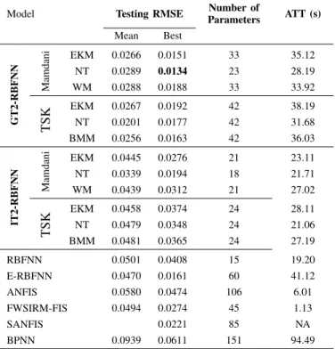
E-RBFNN, it was determined the optimal value to provide a high level of generalisation is with 4 hidden units, where each has 3 fuzzy rules. Table VI shows the average generalisation performance of 20 trials, the number of parameters per each

model as well as the Average Training TimeATTof each GT2

RBFN model with respect to an FWSIRM [38], SANFIS [38], RBFNN, IT2 RBFNN [24], E-RBFNN [39] and the ANFIS system According to Table VI, the highest trade-off between accuracy and model simplicity is obtained by the RBFNN of GT2 using a NT algorithm. From Table VI, it it is clear for most of GT2 RBFNN models the training time is comparable to that of some models such as the BPNN and RBFNN. It is worth noting, the generalisation performance of an E-RBFNN is higher than an IT2 E-RBFNN and similar to a GT2 RBFNN. Both, GT2 RBFNN and E-RBFNN treat uncertainty as measure for ambiguity. However, a GT2 RBFNN quantifies uncertainty as a deficiency that results not only from imprecise boundaries in the fuzzy sets (vagueness or fuzziness), but also as nonspecificity that refers to information-based imprecision, whereas an E-RBFNN defines ambiguity as a variation of the output of the ensemble members over unlabeled data. That means, uncertainty quantification is useful in an ensemble only if there is a disagreement among on some inputs [45].

TABLE VI:COMPARISON OF THE AVERAGE PERFORMANCE OF

20 TRIALS OF DIFFERENT MODELS IN EXAMPLE 2.

Model Testing RMSE _ParametersNumber of ATT (s)

Mean Best GT2-RBFNN Mamdani EKM 0.0266 0.0151 33 35.12 NT 0.0289 0.0134 23 28.19 WM 0.0288 0.0188 33 33.92 TSK EKM 0.0267 0.0192 42 38.19 NT 0.0201 0.0177 42 31.68 BMM 0.0256 0.0163 42 36.03 IT2-RBFNN Mamdani EKM 0.0445 0.0276 21 23.11 NT 0.0339 0.0194 18 21.71 WM 0.0439 0.0312 21 27.02 TSK EKM 0.0458 0.0374 24 28.11 NT 0.0479 0.0348 24 21.06 BMM 0.0481 0.0365 24 27.19 RBFNN 0.0501 0.0408 15 19.20 E-RBFNN 0.0470 0.0161 60 41.12 ANFIS 0.0580 0.0474 106 6.01 FWSIRM-FIS 0.0494 0.0274 45 1.13 SANFIS 0.0221 85 NA BPNN 0.0939 0.0611 151 94.49

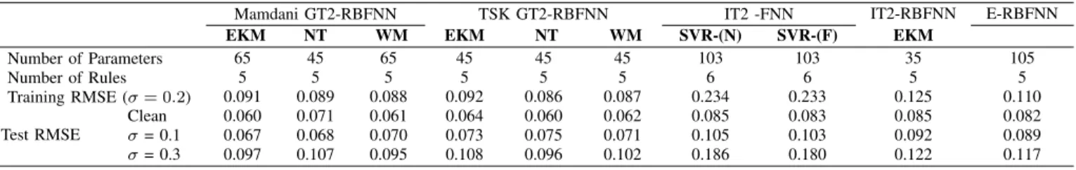
TABLE VII:PERFORMANCE OF THE MAMDANI (TSK) GT2-RBFNN AND OTHER MODELS WITH A TRAINING NOISEσ= 0.2 in example 3.

Mamdani GT2-RBFNN TSK GT2-RBFNN IT2 -FNN IT2-RBFNN E-RBFNN

EKM NT WM EKM NT WM SVR-(N) SVR-(F) EKM

Number of Parameters 65 45 65 45 45 45 103 103 35 105 Number of Rules 5 5 5 5 5 5 6 6 5 5 Training RMSE (σ= 0.2) 0.091 0.089 0.088 0.092 0.086 0.087 0.234 0.233 0.125 0.110 Test RMSE Clean 0.060 0.071 0.061 0.064 0.060 0.062 0.085 0.083 0.085 0.082 σ= 0.1 0.067 0.068 0.070 0.073 0.075 0.071 0.105 0.103 0.092 0.089 σ= 0.3 0.097 0.107 0.095 0.108 0.096 0.102 0.186 0.180 0.122 0.117

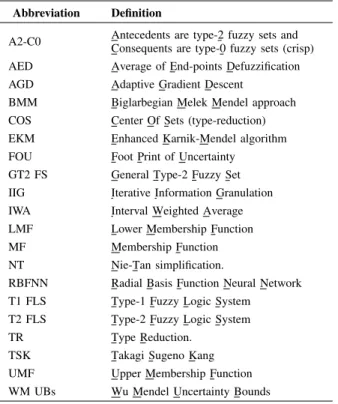
TABLE VIII:PERFORMANCE OF THE MAMDANI (TSK) GT2-RBFNN AND OTHER MODELS WITH A NOISEσ= 0.3in example 3.

Parameters Mamdani GT2-RBFNN TSK GT2-RBFNN IT2 -FNN IT2-RBFNN E-RBFNN

EKM NT WM EKM NT WM SVR-(N) SVR-(F) EKM

Number of Parameters 65 45 65 45 45 45 103 103 35 105 Number of Rules 5 5 5 5 5 5 6 6 5 5 Training RMSE (σ= 0.3) 0.111 0.108 0.122 0.121 0.117 0.114 0.349 0.347 0.133 0.148 Test RMSE Clean 0.085 0.088 0.083 0.079 0.069 0.078 0.127 0.121 0.092 0.120 σ= 0.1 0.109 0.096 0.091 0.081 0.083 0.105 0.138 0.131 0.127 0.132 σ= 0.3 0.125 0.118 0.131 0.133 0.127 0.129 0.188 0.184 0.144 0.159 Number of Data 0 50 100 150 200 y(t+1) -2 -1.5 -1 -0.5 0 0.5 1 1.5 Predicted Output Testing Data

Fig. 15: Testing data, and the output of the GT2-RBFNN with an WM

direct defuzzification and 3 fuzzy rules.

In other words, a GT2 RBFNN can be viewed as an ensemble of interval Type-2 FLSs where all the IT2 FSs

computa-tions occurr for each α-level and ambiguity is nonuniformly

weighted. In this example, a GT2 RBFNN results more practical than an ensemble, especially because it is a more compact model with less parameters and less expensive in terms of computational burden. To exemplify the performance of GT2 RBFNN models, in Fig. 15, the identification result for a GT2 RBFNN with a WM method is shown.

C. Example 3: Noisy Chaotic Time-Series Prediction

As the last experiment, a time-series prediction problem to evaluate the performance of the GT2-RBFNN is employed. The Mackey-Glass chaotic time series is generated from the following differential equation [41]:

dx(t)

dt =

0.2x(t−τ)

1 + 10x(t₋τ)−0.1x(t) (70)

For comparison reasons with previous results, the

parame-ters τ = 30, x(0) = 1.2. Four past values were employed to

predict x(t)where the input data format is used as:

[x(t₋24), x(t₋18), x(t₋12), x(t₋6);x(t)] A number of 1000 patterns were generated from the

obser-vation t = 124 to t = 1123. For cross-validation purposes,

the input data was divided into two subsets, i.e. a) 50% for

training and b)50%for testing. For cross-validation purposes,

two different types of training data were created by adding

Gaussian noise with a standard deviation ofσ= 0.2σ= 0.3

and with a mean of 0 to the original data x(t). This type

of noise has been selected because it usually occurs in real situations and it is frequently employed to verify model robustness [25-29]. For testing data, three data sets were created from the original data set. The first consists of the

original500values. The last two testing data sets were created

by adding a Gaussian noise with a σ= 0.2 and σ= 0.3. To

compare the performance of the GT2-RBFNN to other existing interval type-2 fuzzy modelling methodologies, namely: a) an IT2FNN-SVR-(N), b) an IT2-FNN-SVR-(F) and an c) EKM IT2-RBFNN and d) E-RBFNN. The first two models a) and b) were introduced in [41]. The IT2-FNN-SVR is a six-layer interval type-2 fuzzy neural network with support vector machine regression that uses two different types of input nodes. For the first type, the input nodes in an IT2-FNN-SVR simply forwards each numerical data and is called IT2-FNN-SVR-(N) for short. Thus, the output of the IT2-FNN-IT2-FNN-SVR-(N) is a bounded interval which is described in terms the lower and upper limits of its Footprint Of Uncertainty (FOU). An IT2-FNN-SVR-(F) uses an input node layer that fuzzifies the input numerical data. The third IT2 methodology is an IT2-RBFNN with an EKM approach. And the last methodology is an ensemble of RBFNNs suggested in [39]. According to our experiments, it was determined a number of 3 horizontal slices for an GT2 RBFNN, and 3 hidden units with 3 fuzzy rules each for an E-RBFNN produce the highest balance between model performance and model simplicity. For statistical purposes, each experiment was repeated 10 times, and the RMSE average is used as a comparison performance index. Table VII and VIII show the training and testing results for the prediction of the Mackey-Glass time-series. From Table V, it can be viewed that in general GT2 neural structures outperform the IT2-FNN-SVR and its counterpart the IT2-RBFNN with an EKM. It is also worth noting, the superiority of the GT2-RBFNN is confirmed not only for validation purposes, but also in relation to the number of parameters.

Time step 0 100 200 300 400 500 Output Prediction 0.2 0.4 0.6 0.8 1 1.2 1.4 Mamdani GT2-RBFNN Predicted Output Measured Output

Fig. 16:Testing prediction of a Mamdani GT2-RBFNN with an EKM

type-reduction and a noise level ofσ= 0.3and RMSE = 0.125 that correspond to a training stage with a level of noise ofσ= 0.3.

Hence, the highest accuracy is achieved by a GT2-RBFNN with a WM and NT method respectively. In relation to Table VI, the higher the noise level of the training and testing data, the better the performance of the GT2-RBFNN models with respect to the IT2 fuzzy models. Particularly those GT2 models with an EKM and NT direct defuzzification and of Mamdani type. Finally, in Fig. 16, the testing data-fit of a random experiment using a Mamdani GT2-RBFNN with an EKM and

noise level of σ= 0.3 is illustrated.

VIII. SUMMARY ANDDISCUSSION

From the comparative analysis presented in previous sec-tion, the following summarisation and disscussion is provided: a) By using GT2 FSs, model accuracy of an RBFNN can be improved importantly. Compared to its counterparts the RBFNN and IT2 RBFNN, a higher tradeoff between accuracy and model simplicity is provided. The term

model simplicity is used because compared to other

existing fuzzy models of T1 and T2, a reduced number of fuzzy rules, and hence of parameters is required to obtain similar or better results.

b) Two problems that involve the treatment of randomness

for nonlinear plant identification, and for the prediction of

nosisy chaotic time series was provided. Compared to an

RBFNN of T1 or IT2, a GT2 RBFNN weights uncertainty non uniformly. This allows an RBFNN to better model the effecs of uncertainty. That means, an RBFNN with GT2 FSs quantifies uncertainty as a deficiency that results from imprecise boundaries of the associated FSs, so using GT2 FSs accounts to minimise information-based imprecision. c) From tables IV-VI, column training time is the average time of training epochs spent by each model. As can be noted, the training speed of a GT2 RBFNN with simplified structures is similar to the RBFNN, faster to the ensemble of RBFNNs and similar to the ANFIS model when it comes to modeling large size data sets. d) As illustrated in example 2, a GT2 RBFNN not only

inherits the ability of NNs to approximate complex fun-tions, but also the ability of fuzzy logic models to provide some insights about the system being modelled.

f) By using GT2 FSs usually increases the computational complexity, however this time can be compensated by an improvement in model performance and a model simplification that can be reached by fuzzy structures based on direct-defuzzification algorithms.

e) Further to point f), in terms of computation, the appli-cation of a Gradient Descent approach (GD) to identify

the parameters of a GT2 FLS with KM methods (’or

EKM’) usually results more expensive than the parameter

identification for an RBFNN of T1 or IT2. This is due to the number of iterations that are needed to calculate not only the associated derivatives but also to track the permutations created during the sorting process of any KM method [46]. A GD is usually not globally conver-gent. Thus, a number of optimisation methods based on metaheuristics have been proposed [47]. To make this less severe, in this paper an Adaptive version of a GD approach that includes a momentum term to avoid getting trapped in a local minimum and to speed up the GD convergence is suggested.

IX. CONCLUSIONS

This paper presents a General Type-2 Radial Basis Function Neural Network (GT2 RBFNN) that is functionally equivalent

to a GT2 FLS based on theα₋plane representation, in which

the main inference engine can be viewed as a TSK or Mamdani system. A detailed description of the neural structure and its corresponding parametric optimisation of a GT2-RBFNN with an EKM, and three simplified GT2-RBFNN models that employs three different direct-defuzzification approaches is provided. To offer a comprehensive performance analysis, experimental results about the modelling of ten data sets for multiclass classification and regression problems is provided. Two problems for nonlinear identification and for the predic-tion of chaotic time series in the precense of randomness and Gaussian noise are considered. Based on experimental results, the suggested model is not only able to outperform its counterparts the RBFNN of type-1 and the Interval Type-2 Radial Basis Function Neural Network (IT2 RBFNN), but also to better treat and minimse the effects of uncertainty. It can be also observed from the simulation results that compared to other methodologies, including an ensemble of RBFNNs, the number of parameters of a GT2 RBFNN is usually smaller. Further developments of the GT2 RBFNN may be related with further advances of Type-2 Fuzzy Logic methodologies, Neural Networks and learning. Particularly to reduce the computational complexity and increase model performance. A future study will be also in terms of the evaluation of the GT2 RBFNN to formulate knoweldge in a transparent way to interpretation and analysis of complex systems.

REFERENCES

[1] M. A. Sanchez, O. Castillo, and J. R. Castro, “Generalized type-2 fuzzy systems for controlling a mobile robot and a performance comparison with interval type-2 and type-1 fuzzy systems,” Expert Systems with Applications, vol. 42, no. 14, pp. 5904–5914, 2015.

[2] O. Castillo, L. Amador-Angulo, J. R. Castro, and M. Garcia-Valdez, “A comparative study of type-1 fuzzy logic systems, interval type-2 fuzzy logic systems and generalized type-2 fuzzy logic systems in control problems,”Information Sciences, vol. 354, pp. 257–274, 2016.