Uncertainty-aware sensor deployment strategy in mixed wireless sensor networks

(1)

Chang, Y., Zhang, S., Zhang, Y., Fan, J., and Wang, J. (2013)

Uncertainty-aware sensor deployment strategy in mixed wireless sensor

networks.

International Journal of Distributed Sensor Networks, 2013 . p.

834704. ISSN 1550-1329

Copyright © 2013 The Authors

http://eprints.gla.ac.uk/96381/

Deposited on: 28 August 2014

Enlighten – Research publications by members of the University of Glasgow

http://eprints.gla.ac.uk

(2)

Hindawi Publishing Corporation

International Journal of Distributed Sensor Networks Volume 2013, Article ID 834704,9pages

http://dx.doi.org/10.1155/2013/834704

Research Article

Uncertainty-Aware Sensor Deployment Strategy in Mixed

Wireless Sensor Networks

Yan Chang,

1

Shukui Zhang,

1,2

Yang Zhang,

3

Jianxi Fan,

1

and Jin Wang

1

1_{School of Computer Science and Technology, Soochow University, Suzhou 215006, China}

2_{State Key Laboratory for Novel Software Technology, Nanjing University, Nanjing 210093, China}

3_{School of Engineering, University of Glasgow, Glasgow, G12 8QQ, UK}

Correspondence should be addressed to Shukui Zhang; [email protected] Received 13 July 2013; Accepted 22 September 2013

Academic Editor: Zhijie Han

Copyright © 2013 Yan Chang et al. This is an open access article distributed under the Creative Commons Attribution License, which permits unrestricted use, distribution, and reproduction in any medium, provided the original work is properly cited. Deployment is a fundamental issue in wireless sensor networks (WSNs), which affects the performance and lifetime of the networks. Usually the sensor locations are precomputed based on “perfect” sensor detection model, whereas sensors may not always provide reliable information, either due to operational tolerance levels or environmental factors. Therefore, it is very important to take into account this uncertainty in the deployment process. In this paper, we address the problem of sensor deployment in a mixed sensor network where the mobile and static nodes work collaboratively to perform deployment optimization task. We consider the Gaussian white noise in the environment and present a centralized algorithm (FABGM for short) which discoveres vacancies by using detection model based on false alarm and moves the mobile nodes according to the method based on bipartite graph matching in this study. In this algorithm, the management node of the WSNs collects the geographical information of all of the static and mobile sensors. Then, the management node executes the algorithm to get the best matches between mobile sensors and coverage holes. Simulation results are presented to demonstrate the effectiveness of the proposed approach.

1. Introduction

Wireless sensor networks have received intensive research interest in recent years due to their potential capability of monitoring real physical environments and collecting data. WSNs have been used in various applications, such as forest monitoring, precision agriculture [1], battlefield surveillance, and target tracking. However, in order to conduct their tasks successfully, it is very important that they be deployed properly.

Sensor deployment is at the initial stages in sensor net-works research. It is an important issue which has attracted much attention in recent years [2]. The number and locations of sensors deployed in a Region of Interest (RoI) determine the topology of the network, which will further influence many of its intrinsic properties, such as its coverage, connec-tivity, cost, and lifetime. Consequently, the performance of a sensor network depends to a large extent on its deployment. A problem which impinges upon the success of any WSNs deployment is the fact that sensory data are marred by the

flaw of uncertainty. Indeed, information provided by sensors may not always reliable, either due to environmental factors such as Gaussian white noise or operational tolerance levels. Therefore, it is very important to take into account this uncertainty in the deployment process.

However, WSNs cannot be deployed manually in many working environments, such as remote mountainous regions, battlefields, and regions polluted by poisonous gases. An alternative method is scattering the sensors randomly, but this is affected by many uncontrollable factors, and it is difficult to achieve the desired deployment. In the last decade, researchers have focused on mixed sensor networks, in which the static nodes and mobile nodes work in a collaborative fashion to perform deployment task. Such networks have the advantage of mobility so they can be moved to appropriate positions to enhance the extent of coverage and reduce the number of nodes.

In this work, we explore the problem of uncertainty-aware deployment in mixed wireless sensor networks. The original contributions of this work are the following: first, we

(3)

introduce a false alarm based detection model; a model con-siders the existence of Gaussian white noise. Second, using the detection model we compute joint detection probability to discover the coverage vacancies. And then, we present an approach which is based on bipartite graph matching to determine the position of the mobile sensor nodes. Before a mobile node moves to coverage vacancy, it will determine whether there are static nodes within its sensing range. If there are static nodes within its sensing range, it moves to the coverage vacancy. Otherwise, it remains in its current position. Experimental results are given to demonstrate the efficiency of our approach.

The remainder of this paper is organized as follows.

Section 2explains related works.Section 3gives an overview

of the false alarm based detection model, and we detail our deployment algorithm inSection 4. Section 5presents our experiments. This paper is concluded inSection 6.

2. Related Prior Works

According to the characteristics of the nodes that comprise WSNs, there are three types of such networks, that is, (1) static WSNs, in which all the nodes are static; (2) mobile WSNs, in which all the sensors are mobile; and (3) mixed WSNs, in which some of the nodes are static and some are mobile.

The greatest weakness of a random static WSN is that there must be significant redundancy among the nodes in order to achieve good coverage. And the deployment of a deterministic static WSN is inefficient. In [3], the authors use a sequential deployment of sensors that is, a limited number of sensors; are deployed in each step until the desired probability of detection of a target is achieved. Sensor place-ment on two- and three-dimensional grids was formulated as a combinatorial optimization problem and solved using integer linear programming [4]. The main drawbacks of these approaches are that the grid coverage approach relies on “perfect” sensor detection; that is, a sensor is expected to yield a binary yes/no detection outcome in every case. The authors in [5] provide a polynomial-time, greedy, iterative algorithm to determine the best placement of one sensor at a time in a grid based scenario, such that each grid is covered with a minimum confidence level. Uncertainty associated with the predetermined sensor locations is considered in [6]. The authors propose two sensor placement algorithms, where the sensor location is modeled as a random variable with a Gaussian probability distribution. In [7, 8], the authors define an evidence-based coverage model and conceive an uncertainty-aware deployment algorithm, which determines the minimum number of sensors and their locations to ensure full area coverage. The evidence-based sensor coverage model is a generalization of the probabilistic model.

In mobile WSNs, a fundamental issue is the coverage problem. Many techniques have been developed to deal with this issue, such as coverage pattern-based movement [9–12], virtual force-based movement [13, 14], and Voronoi-based movement [15]. A distributed energy-efficient deployment algorithm is proposed by Heo and Varshney [9]. The goal is the formation of an energy-efficient node topology for a

longer system lifetime. In order to achieve this goal, they employ a synergistic combination of cluster structuring and a peer-to-peer deployment scheme. Moreover, an energy-efficient deployment algorithm based on Voronoi diagrams is also proposed here. The authors in [13] propose a deployment strategy to enhance coverage after an initial random place-ment of sensors using virtual forces. A cluster head computes the new locations of all the sensors after an initial deployment that would maximize coverage, and then nodes reposition themselves to the designated locations. Wang et al. [15] use Voronoi diagrams to discover the coverage vacancies and design three movement-assisted sensor deployment proto-cols, including VEC (vector based), VOR (Voronoi based), and minimax. The greatest weakness of a mobile WSN is its price, which is significantly greater than the price of a static WSN, because the price of mobile sensors is much greater than the price of static sensors.

The mixed wireless sensor networks that are composed of a mixture of mobile and static sensors are the tradeoff between cost and coverage. To provide the required high coverage, the mobile sensors have to move from dense areas to sparse areas. In [16], the authors proposed a collaborative coverage enhancing algorithm (coven) which uses a “Voronoi polygon” to determine the placed positions and the number of estimated holes. However, it is not feasible to apply Voronoi diagrams in WSNs due to their excessive complexity. A grid deployment method is proposed in [17], where the map is divided into multiple individual grids, and the weight of each grid is determined by environmental factors such as predeployed nodes, boundaries, and obstacles. The grid with minimum values is the goal of the mobile node. The authors in [18] proposed a novel, centralized algorithm to deploy a mixture of mobile and static sensors to construct sensor networks which used Delaunay triangulation rather than a Voronoi diagram to detect the coverage holes.

To the best of our knowledge, almost all related works assume either a binary or a probabilistic-based coverage model. The binary coverage model is overly simplistic and does not reflect reality, while the probabilistic coverage model is limited and does not allow the easy integration of some related issues, such as sensor reliability. This paper presents a centralized algorithm in which the management node executed the algorithm to discover vacancies by using detection model based on false alarm and then to get the best matches between mobile sensors and coverage holes. The detection model used in our work considers the environment factor and reflects reality well. Simulation results show the effectiveness of our algorithm.

3. Detection Model

3.1. Assumptions. Our algorithm is based on the following

assumptions.

(i) The location of each sensor node is known, which can be obtained at a low cost from Global Positioning Sys-tem (GPS) or through location discovery algorithms. (ii) It is assumed that all sensor nodes have identical

(4)

International Journal of Distributed Sensor Networks 3 (iii) The mobile nodes have the ability to move and can

move to the optimized position accurately.

3.2. Sensor Detection Model. We assume that the WSNs work

in an environment with a Gaussian white noise, and each sensor involved in the signal detection transmits a signal with the same energy𝑒_tr. Thus, the signal received at a distance of𝑟meters away will have energy of𝑒_tr/𝑟𝛾. Here, a simple geometric path loss model [19] is assumed, and the path loss is proportional to1/𝑟𝛾, where𝛾is the path loss exponent, which is an environment-dependent constant typically between 2 and 4. We assume that the number of sensors which perform signal detection is𝑛. Thus, at sensor𝑖, the observations under the two different hypotheses are given by [20]

𝑦_𝑖={{_{_{ { 𝛽 𝐷𝛾/2_𝑡𝑖 + 𝑛𝑖 𝐻1, 𝑖 = 1, 2, . . . , 𝑛, 𝑛_𝑖 𝐻₂, 𝑖 = 1, 2, . . . , 𝑛, (1)

where𝐻₁ denotes the target-present hypothesis, and𝐻₀ is the null hypothesis;𝑦_𝑖is the received signal;𝑛_𝑖is zero-mean, complex Gaussian noise with variance𝜎2;𝛽is a scalar defined

by𝛽 = √𝑒_tr/2𝛾; and𝐷_𝑡𝑖denotes the distance between the

target(𝑥_𝑡, 𝑦_𝑡)and the sensor(𝑥_𝑖, 𝑦_𝑖); that is,

𝐷𝑡𝑖= √(𝑥𝑡− 𝑥𝑖)2+ (𝑦𝑡− 𝑦𝑖)2. (2)

It is noted that under hypothesis 𝐻₁, the distance that the active sensing signal traverses is given by 𝑟 = 2𝐷_𝑡𝑖. Therefore, for the 𝑖th sensor, the likelihood (probability density function) under𝐻₁is given by

Pr(𝑦_𝑖| 𝐻₁) = 1 √2𝜋𝜎2exp { { { − 1 2𝜎2(𝑦𝑖− 𝛽 𝐷𝛾/2_𝑡𝑖 ) 2_} } } , (3)

and the likelihood under𝐻₀is Pr(𝑦_𝑖| 𝐻₀) = 1

√2𝜋𝜎2 exp{−

𝑦_𝑖2

2𝜎2} . (4)

Now, let us focus on the Neyman-Pearson criterion. The Neyman-Pearson criterion maximizes the probability of detection𝑃_𝐷 subject to a predetermined bound on the probability of false alarm 𝑃_𝐹. In other words, the optimal decision rule𝜗according to the Neyman-Pearson criterion is the solution to the following constrained optimization problem [21]:

max

𝜗 𝑃𝐷(𝜗) subject to𝑃𝐹(𝜗) ≤𝛼. (5)

The Neyman-Pearson optimum test is a likelihood ratio test [13]. From (3) and (4), the likelihood ratio for sensor𝑖can be written as 𝐿_𝑖(𝑦_𝑖) =𝑃𝑟(𝑦𝑖| 𝐻1) 𝑃_𝑟(𝑦_𝑖| 𝐻₀) =exp{ 1 2𝜎2( 2𝛽𝑦_𝑖 𝐷𝛾/2_𝑡𝑖 − 𝛽2 𝐷𝛾_𝑡𝑖)} . (6)

Since the𝑛_𝑖, 𝑖 ∈ [1, 𝑛], are assumed to be statistically inde-pendent, the joint probability of the observations is simply the product of the individual probability densities. Thus, let us define 𝑦 = [𝑦₁, . . . , 𝑦_𝑛], for the 𝑛 sensors, the overall likelihood ratio is

𝐿 (𝑦) =∏𝑛

𝑖=1

𝐿_𝑖(𝑦_𝑖) . (7)

For convenience, we consider the log-likelihood ratio, which is given by ln𝐿 (𝑦) = 𝑛 ∑ 𝑖=1 ln𝐿_𝑖(𝑦_𝑖) = 1 2𝜎2 𝑛 ∑ 𝑖=1 (2𝛽𝑦𝑖 𝐷𝛾/2_𝑡𝑖 − 𝛽2 𝐷𝛾_𝑡𝑖) . (8)

Therefore, the likelihood ratio test is given by [21]

1 2𝜎2 𝑛 ∑ 𝑖=1 (2𝛽𝑦𝑖 𝐷𝛾/2_𝑡𝑖 − 𝛽2 𝐷𝛾_𝑡𝑖) ≥ln𝜂 𝐻1, 1 2𝜎2 𝑛 ∑ 𝑖=1 (2𝛽𝑦𝑖 𝐷𝛾/2_𝑡𝑖 − 𝛽2 𝐷𝛾_𝑡𝑖) <ln𝜂 𝐻0, (9)

where𝜂is uniquely determined by solving𝑃_𝐹 = 𝛼. Equiva-lently, we can reformulate (9) into

𝑛 ∑ 𝑖=1 𝑦𝑖 𝐷𝛾/2_𝑡𝑖 ⏟⏟⏟⏟⏟⏟⏟⏟⏟⏟⏟⏟⏟ 𝑔 ≥_𝛽1𝜎2ln𝜂 + 1 2 𝑛 ∑ 𝑖=1 𝛽 𝐷𝛾_𝑡𝑖 ⏟⏟⏟⏟⏟⏟⏟⏟⏟⏟⏟⏟⏟⏟⏟⏟⏟⏟⏟⏟⏟⏟⏟⏟⏟⏟⏟⏟⏟⏟⏟⏟⏟⏟⏟ 𝜏 𝐻₁, 𝑛 ∑ 𝑖=1 𝑦_𝑖 𝐷𝛾/2_𝑡𝑖 ⏟⏟⏟⏟⏟⏟⏟⏟⏟⏟⏟⏟⏟ 𝑔 < 1 𝛽𝜎2ln𝜂 + 1 2 𝑛 ∑ 𝑖=1 𝛽 𝐷𝛾_𝑡𝑖 ⏟⏟⏟⏟⏟⏟⏟⏟⏟⏟⏟⏟⏟⏟⏟⏟⏟⏟⏟⏟⏟⏟⏟⏟⏟⏟⏟⏟⏟⏟⏟⏟⏟⏟⏟ 𝜏 𝐻₀, (10)

where we have further defined the test statistics𝑔and the new threshold𝜏. For a fixed set of sensors, the second part of𝜏 will be fixed and known. The variable𝑔is actually asufficient

statistic, and when making a decision, knowing the value of𝑔

will be just as good as knowing𝑦. Then, invoking the model for𝑛_𝑖, the hypothesis pair can be written as

𝐻₀: 𝑔 ∼ 𝑁 (0,∑𝑛 𝑖=1 𝜎2 𝐷𝛾_𝑡𝑖) versus 𝐻₁: 𝑔 ∼ 𝑁 (∑𝑛 𝑖=1 𝛽 𝐷𝛾_𝑡𝑖, 𝑛 ∑ 𝑖=1 𝜎2 𝐷𝛾_𝑡𝑖) . (11)

For notational convenience, let us define

𝜇₁=∑𝑛 𝑖=1 𝛽 𝐷𝛾_𝑡𝑖, 𝜎 2 1 = 𝑛 ∑ 𝑖=1 𝜎2 𝐷𝛾_𝑡𝑖. (12)

(5)

Thus, the false alarm probability is 𝑃_𝐹=Pr(𝑔 > 𝜏 | 𝐻₀) =Pr(𝑔 𝜎₁ > 𝜏 𝜎₁ | 𝐻0) = 1 − Φ (_𝜎𝜏 1) , (13)

whereΦ(⋅)is the standard Gaussian cumulative distribution function; that is,

Φ (𝑧) = ∫𝑧 −∞ 1 √2𝜋exp(− 𝑧2 2) 𝑑𝑧. (14)

Similarly, the detection probability is given by

𝑃_𝐷=Pr(𝑔 > 𝜏 | 𝐻₁) =Pr(𝑔 − 𝑢1 𝜎₁ > 𝜏 − 𝑢₁ 𝜎₁ | 𝐻1) = 1 − Φ (𝜏 − 𝜇1 𝜎₁ ) . (15)

It is clearly seen that with the aid of (11), the false alarm probability𝑃_𝐹, the detection probability𝑃_𝐷, and the detection threshold𝜏(or𝜂) are connected by some one-to-one rela-tions. Suppose that we define the allowed level of false alarm as𝑃_𝐹= 𝛼, then from (13), we obtain

𝜏

𝜎1 = Φ

−1_{(1 − 𝛼) .}

(16) By the definitions of𝜇₁and𝜎₁in (12), we can write

𝜇₁ 𝜎₁ = 𝛽 𝜎( 𝑛 ∑ 𝑖=1 1 𝐷𝛾_𝑡𝑖) 1/2 . (17)

Therefore, by using (16) and (17), we can reformulate𝑃_𝐷of (15) into 𝑃𝐷= 1 − Φ (Φ−1(1 − 𝛼) −𝛽_𝜎( 𝑛 ∑ 𝑖=1 1 𝐷𝛾_𝑡𝑖) 1/2 ) . (18)

We assume that the target may appear at a random position

𝑘 in the detection area. By using (18), we can obtain the detection probability of the target at any position𝑘.

Consider 𝐶_𝑘(𝑃) = 1 − Φ (Φ−1(1 − 𝛼) −𝛽_𝜎(∑𝑛 𝑖=1 1 𝐷𝛾_𝑘𝑖) 1/2 ) , (19)

where𝑛denotes the number of nodes which is deployed in the detection area. Here,𝐷_𝑘𝑖 denotes the distance between the point𝑘(𝑥_𝑘, 𝑦_𝑘)and the𝑖th sensor(𝑥_𝑖, 𝑦_𝑖); that is, by using (19), we can formulate the detection probability of any point

𝑘in the detection area.

4. Deployment Algorithm

In this paper, we evaluate the coverage performance by area coverage rate. We assume that𝑁static nodes and𝑀 mobile nodes are deployed in the𝐿 × 𝐿area. The𝐿 × 𝐿m2 square monitored area is divided into𝐿 × 𝐿small uniform square grids. Each grid has the same length of 1 m. For simplicity, here we transform the area coverage problem of WSN into grid coverage problem. We compute joint detection probability𝐶_𝑘(𝑃)of the center point of grid𝑘and use the detection probability𝐶_𝑘(𝑃)to measure whether each grid is covered. The area coverage rate is defined as the ratio between the coverage area𝐴area(𝑃)of the node set and the total area

𝐴_𝑠of the detection region. Thus, the area coverage rate is

𝑅area(𝑃) =𝐴area_𝐴(𝑃)

𝑠 =

∑𝐿×𝐿_𝑘=1𝐶_𝑘(𝑃)

𝐿 × 𝐿 . (20)

4.1. The Discovery of Coverage Vacancies. At first,𝑛sensors

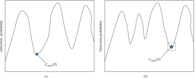
(include 𝑁 static nodes and 𝑀 mobile nodes) have been scattered randomly in a𝐿 × 𝐿area. After the initial random deployment of the sensor nodes, the distribution function of the detection probability of the nodes approximates to exponential form. In the two-dimensional detection area, we can obtain the joint detection probability of any grid 𝑘in the detection region by the sensor detection model based on false alarm (19). Then, we will search grids at𝐶_min(𝑃)(see

Figure 1). The𝑀(the number of mobile nodes) girds which

have the lowest detection probability are defined as coverage vacancies. Since the detection probability of each position is continuous, the probability around the point which has lower probability is also low. Thus, moving the mobile nodes to the coverage vacancies can improve the coverage performance of the network. Repeating this process until the iteration times𝑡 reaches the preset value (𝑡pre) or 𝐶min(𝑃)achieves

satisfactory probability(𝑃_𝑠). In order to avoid that the moving distance of a single node is too large, we deploy virtual nodes at the position of coverage vacancies per iteration. When the iteration process terminates, we move the mobile nodes to the position of virtual nodes.

4.2. The Movement of Mobile Nodes. After the termination

of iteration, the position of the virtual nodes is defined as coverage vacancies. For the initial network deployment, Firstly we construct a bipartite graph𝐺 = (𝑉, 𝐸),𝑉 = 𝑉₁∪ 𝑉₂, where𝑉₁denotes the set of mobile nodes and𝑉₂denotes the set of virtual nodes. We take the moving distance as cost to illustrate the construction method of the bipartite graph. The concrete method is given by the following.

(1) Add all the movable nodes into𝑉₁. (2) Add all the virtual nodes into𝑉₂.

(3) For∀𝑢 ∈ 𝑉₁and∀]∈ 𝑉₂, if mobile node𝑢can reach

V, (the distance between𝑢andVdoes not exceed the maximum moving distance𝑑_𝑢of𝑢or the remaining energy of𝑢 is within a certain range𝐸residual) then

add an edge(𝑢,V)into the bipartite graph; the weight of the edge(𝑢,V)which is defined as𝑤(𝑢,V)denotes

(6)

International Journal of Distributed Sensor Networks 5 D et ec tio n pro babi lit y Cmin(P) (a) D et ec tio n pro babi lit y Cmin(P) (b)

Figure 1: Schematic of joint detection probability. (a) Detection probability before iteration. (b) Detection probability after iteration.

the distance between sensor node𝑢and virtual node

V, otherwise,𝑤(𝑢,V) = 0.

A set𝐻of independent edges in a graph𝐺 = (𝑉, 𝐸)is called a matching (see [22]).𝐻is a matching of𝑈 ⊆ 𝑉if every vertex in𝑈is incident with an edge in𝐻. The vertices in𝑈 are then called matched (by𝐻); vertices not incident with any edge of𝐻are unmatched. Because the two ends of any edge of𝐺lie in different set of vertices, the number of edges in

𝐻denotes that|𝐻|virtual nodes (that is coverage holes) are covered by|𝐻|mobile nodes. Corresponding cost is given by

𝐶_𝐻= ∑_(𝑢,V)𝑤(𝑢,V). Thus, maximizing the network coverage

and minimizing the moving distance in this condition can be transformed into a problem of finding a maximum matching

𝐻optof bipartite graph𝐺which has a minimum cost, that is,

for any matching𝐻of𝐺,|𝐻| ≤|𝐻opt|; If|𝐻| = |𝐻opt|, then

𝐶(𝐻) ≥ 𝐶(𝐻opt). A maximum matching 𝐻opt of bipartite

graph𝐺which has a minimum cost represents an optimal mobile solution. Deploying the mobile nodes according to the optimal mobile solution, the coverage of the network can be improved while the moving distance is the smallest.

For illustration, an example is given here. We assume that the vertex set of bipartite graph 𝐺 is 𝑉 = 𝑉₁ ∪ 𝑉₂. The mobile node set𝑉₁ = {𝑥₁, 𝑥₂, 𝑥₃, 𝑥₄, 𝑥₅}, and virtual node set𝑉₂= {𝑦₁, 𝑦₂, 𝑦₃, 𝑦₄, 𝑦₅}. Here, we just consider movement distance. As introduced above, if the distance between𝑥_𝑖and

𝑦_𝑗does not exceed the maximum moving distance𝑑_𝑥𝑖of𝑥_𝑖, it indicates that mobile node𝑥_𝑖can reach𝑦_𝑗, then add an edge

(𝑥_𝑖, 𝑦_𝑗)into the bipartite graph𝐺.The weight of edge(𝑥_𝑖, 𝑦_𝑗) is defined as 𝑤(𝑥_𝑖, 𝑦_𝑗) which denotes the distance between sensor node𝑥_𝑖and virtual node𝑦_𝑖; otherwise,𝑤(𝑢,V) = 0. Otherwise, add an edge whose weight is 0 into the bipartite graph𝐺. For example, if the distance between𝑥₁and𝑦₁is 3, it is assumed that the maximum moving distance of𝑥₁is 10, then add an edge(𝑥₁, 𝑦₁)whose weight is 3 into the bipartite graph𝐺. Similarly, we can obtain the weight of other edges of bipartite𝐺, as shown inFigure 2(a). After the construction of the bipartite graph 𝐺, then we can obtain a maximum matching𝐻optof bipartite graph𝐺which has a minimum cost

𝐻opt= {𝑥1𝑦5, 𝑥2𝑦3, 𝑥3𝑦4, 𝑥4𝑦2, 𝑥5𝑦1}. 3 5 5 4 1 2 2 0 2 2 2 4 4 1 0 0 1 1 0 0 1 2 1 3 3 x1 x2 x3 x4 x5 y1y2y3y4y5 (a) x1 x2 x3 x4 x5 y1 y2 y3 y4 y5 (b)

Figure 2: An example of bipartite graph construction (a) Weight matrix of edges of bipartite graph (b) the constructed bipartite graph.

Table 1: Settings of simulation parameter.

Parameter Value

The area of𝐴_𝑠 80 × 80m2

The iteration times𝑡 30

Total number of nodes:𝑛 60

The value of𝛾 2

The value of𝜎 1

The value of𝛽 7

The value of𝑃_𝐹= 𝛼 5%

According to𝐻opt, we will move𝑥₁to𝑦₅, 𝑥₃to𝑦₄, 𝑥₄to𝑦₂, and𝑥₅to𝑦₁, respectively. For𝑤(𝑥₂, 𝑦₃) = 0, we do not move node𝑥₂. The corresponding cost is 4. The concrete algorithm is as found inAlgorithm 1.

5. Simulations Results

Now we present simulation results regarding the proposed algorithm. All of the simulation results given in the following are obtained by programs in C++ and Matlab. We consider a specific WSNs scenario where the field has a square shape of

size80 × 80m2; 60 sensor nodes (including static and mobile

nodes) are randomly distributed over this field. We ran 100 simulations for every result and calculated the average result. The experimental parameters are shown inTable 1.

(7)

input: Static nodes𝑆 = {𝑠₁, 𝑠₂, . . . , 𝑠_𝑁}, Mobile nodes𝑉₁= {V₁,V₂, . . . ,V_𝑀},𝐸_residual,𝑑_𝑢,𝑢 ∈ 𝑉₁,𝑡_pre,𝑃_𝑠 False-alarm probability parameter𝛼, 𝛽, 𝛾, 𝜎, 𝑒_tr

Output:

(1) 𝑡 ← 0.

(2) Calculate𝐶_𝑘(𝑃)of the target at any position𝑘of area𝐴_𝑠using (19). (3) Repeat:

(4) Search𝐶_min(𝑃), construct set of virtual node𝑉₂={(𝑥_𝐸,1, 𝑦_𝐸,1), (𝑥_𝐸,2, 𝑦_𝐸,2), . . . , (𝑥𝐸,𝑀, 𝑦𝐸,𝑀)}.

(5) Update the static node set𝑆 = {𝑠₁, 𝑠₂, . . . , 𝑠_𝑁} ∪ 𝑉₂. (6) Update iteration times, set𝑡:𝑡 = 𝑡 + 1.

(7) Calculate𝐶_𝑘(𝑃)of the target at any position𝑘of area𝐴_𝑠using (19). (8) Until (iteration time𝑡is larger than𝑡preor𝐶min(𝑃)is larger than𝑃𝑠) (9) Construct bipartite graph𝐺 = (𝑉, 𝐸), calculate𝐻opt.

(10) Adjust the position of the mobile nodeV_𝑖,V_𝑖∈ 𝑉₁according to optimal mobile solution which is in consistent with𝐻opt.

Algorithm 1: Algorithm FABGM.

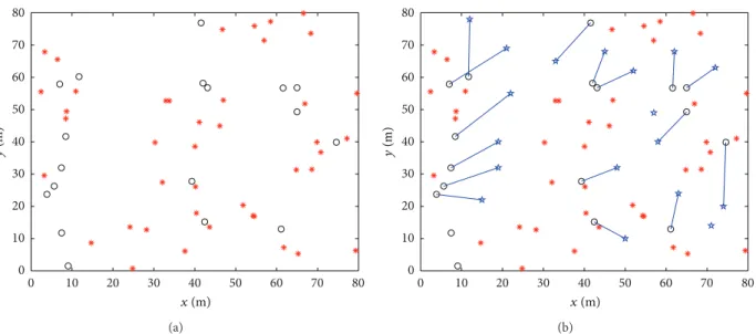
0 10 20 30 40 50 60 70 80 0 10 20 30 40 50 60 70 80 x(m) y (m) (a) 0 10 20 30 40 50 60 70 80 0 10 20 30 40 50 60 70 80 x(m) y (m) (b) Figure 3: Position of mobile nodes before and after optimization.

Figure 3 shows the schematic diagram of movement

condition of the mobile nodes. The circle represents the mobile node and the five-pointed star represents coverage void. If a circle𝑖and a five-pointed star𝑗are connected by a line, it indicates that mobile node represented by circle𝑖can move to the coverage hole represented by the five-pointed star

𝑗. As introduced above, if the distance between mobile node

𝑢and coverage holeVexceeds the maximum moving distance

𝑑_𝑢of𝑢or the remaining energy of𝑢is less than a preset value

𝐸residual, we set𝑤(𝑢,V) = 0. Thus, according to practical

situ-ation, we can set different𝑑_𝑢and𝐸residual, then we can obtain

a different weight matrix regarding edges of the constructed bipartite graph and different optimal mobile solutions. There-fore, the proposed algorithm is more flexible and reflects reality well. After performing FABGM algorithm, the sensors are distributed uniformly in the detection area, which helps to increase the system efficiency, improve energy conservation, and decrease the probability of missing an event.

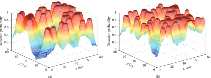
Figure 4 provides the schematic diagram of detection

probability distribution comparison between the random method and our deployment method. It is obvious that there are many coverage vacancies and points with low probability in the network after the initial random deployment. From

Figure 4(b), we know that the proposed algorithm in this

paper can decrease the coverage void and improve the coverage performance of the network. Figure 5shows the coverage performance of FABGM algorithm when the mobile nodes percentage varies from 0% to 80%. Due to the lack of reference system, we compare the proposed algorithm with the initial deployment. We can see that our deployment can enhance coverage compared to the initial random deploy-ment and that the network coverage quality increases with the number of mobile nodes increase. However, when the mobile node percentage is larger than 50%, network coverage increases slowly along with the increase of the number of mobile nodes.

(8)

International Journal of Distributed Sensor Networks 7 0 20 40 60 80 0 20 40 60 800 0.2 0.4 0.6 0.8 1 D et ec tio n pro babi lit y 60 60 x(m) y_(m) (a) 0 20 40 60 80 0 20 40 60 800 0.2 0.4 0.6 0.8 1 D et ec tio n pro babi lit y x(m) y_(m) 60 (b)

Figure 4: Distribution of joint detection probabilities. (a) Random deployment. (b) Distribution after running FABGM.

80 85 90 95 100 0 10 20 30 40 50 60 70 80 C o ve rag e (%)

Number of mobile nodes (%) Initial coverage

False-alarmed algorithm

Figure 5: Coverage quality before and after optimization.

In order to analyze the relationship between coverage performance and the value of 𝛽, we discuss the network coverage condition when the value of 𝛽 is 1, 3, 6, and 8 separately. FromFigure 6, we know that when the value of

𝛽is fixed, the network coverage improves with the increase of number of mobile nodes. When the value of𝛽is small, the network coverage improves apparently. When the value of𝛽is large (e.g., = 6, 8), increasing the number of mobile nodes will not improve network coverage significantly. That is because the value of𝛽is proportionate to 𝑒_tr when 𝛾 is fixed, when the value of𝛽is large,𝑒_tris also large. It indicates that each sensor node consumes much energy to transmit signal, so its detection range increases. The initial deployed sensors can almost cover the whole area, and so increasing the number of mobile nodes does not enhance network coverage significantly. The value of𝛽can be determined according to practical application.

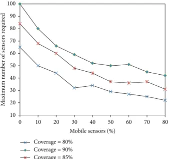
Figure 7gives the minimum number of sensors required

to reach a certain coverage percent when the percentage of mobile sensors varies from 0% to 80%, in 10% increments. As shown inFigure 7, the sensor nodes required in the mixed

0.2 0.3 0.4 0.5 0.6 0.7 0.8 0.9 1 0 10 20 30 40 50 60 70 80 C o ve rag e (%) Mobile nodes (%) 𝛽 = 1 𝛽 = 3 𝛽 = 6𝛽 = 8

Figure 6: Coverage comparison of different𝛽.

WSN are less than that in the static WSN. As the percentage of mobile sensors is 40%, the number of sensors in the mixed WSN is about half the number of sensors in the static WSN. The number of sensors needed decrease with the increase of the number of mobile nodes. When the percentage of mobile sensors increases from 0% to 30%, the number of sensors for 80% coverage decreases from 65 to 35, but when the percentage increases from 50% to 70%, the effect is not as significant as before. Considering that the price of mobile sensors is higher than the price of static sensors, it is necessary to determine proper number of mobile nodes in a network. However, the number of mobile nodes is related to the ratio of the price of mobile sensors to the price of static sensors.

Figure 8shows the cost of WSN to reach 85% coverage

at different ratios of the price of mobile sensors to the price of static sensors. When the price discrepancy of mobile nodes and static nodes is minor, increasing the proportion of mobile

(9)

10 20 30 40 50 60 70 80 90 100 0 10 20 30 40 50 60 70 80 M axim um n u m b er o f s en so rs r eq u ir ed Mobile sensors (%) Coverage = 80% Coverage = 85% Coverage = 90%

Figure 7: The minimum number of sensors required to reach a coverage percent in different mobile percentages.

0 100 200 300 400 500 600 0 10 20 30 40 50 60 70 80 The cost o f W SN Mobile sensors (%) Mobile/static = 1.5 Mobile/static = 2 Mobile/static = 3.5 Mobile/static = 6 Mobile/static = 9.5

Figure 8: The cost to reach 85% coverage.

sensors can reduce the overall cost of WSN. When the ratio is between 2 and 6, the mixed WSN has the lower cost, and also the proportion of mobile sensors is not very high (e.g., 20%≤ the percentage of mobile sensors≤50%). But when the ratio is greater than 6, it is better that the nodes in the network are all static nodes. It is apparent that the mixed WSN is a best choice when the ratio between the price of the mobile sensor and the price of the static sensor is 2–6. Under this circumstance, our proposed algorithm is useful and can provide a tradeoff between the cost and the coverage.

6. Conclusion

Sensor deployment is at the initial stages in sensor networks research. Here, we explore the problem of uncertainty-aware WSNs deployment, and we start with a “random” distribution of the nodes (including mobile nodes and static nodes) over

the region of interest. In this paper, we propose a false-alarm deployment algorithm to improve an initial deployment of nodes. After going through the proposed algorithm, the area of interest is covered by uniformly nodes. Simulation results demonstrate the effectiveness of the proposed approach.

Acknowledgments

This work is supported by National Natural Science Founda-tion of China under Grants No. 61070169 and Natural Science Foundation of Jiangsu Province under Grant no. BK2011376, the Specialized Research Foundation for the Doctoral Pro-gram of Higher Education of China No. 20103201110018 and Application Foundation Research of Suzhou of China No. SYG201118, SYG201240.

References

[1] M. Mafuta, M. Zennaro, A. Bagula, G. Ault, H. Gombachika, and T. Chadza, “Successful deployment of a wireless sensor network for precision agriculture in malawi,” International Journal of Distributed Sensor Networks, vol. 2013, Article ID 150703, 13 pages, 2013.

[2] B. Wang,Coverage Control in Sensor Networks, Springer, New York, NY, USA, 2010.

[3] T. Clouqueur, V. Phipatanasuphorn, P. Ramanathan, and K. K. Saluja, “Sensor deployment strategy for target detection,” in Proceedings of the 1st ACM International Workshop on Wireless Sensor Networks and Applications, pp. 42–48, New York, NY, USA, September 2002.

[4] K. Chakrabarty, S. S. Iyengar, H. Qi, and E. Cho, “Grid coverage for surveillance and target location in distributed sensor networks,”IEEE Transactions on Computers, vol. 51, no. 12, pp. 1448–1453, 2002.

[5] S. S. Dhillon, K. Chakrabarty, and S. S. Iyengar, “Sensor placement for grid coverage under imprecise detections,” in Proceedings of the 5th International Conference on Information Fusion, vol. 2, pp. 1581–1587, 2002.

[6] Y. Zou and K. Chakrabarty, “Uncertainty-aware sensor deploy-ment algorithms for surveillance applications,” inProceedings of the IEEE Global Telecommunications Conference (GLOBECOM ’03), pp. 2972–2976, December 2003.

[7] M. R. Senouci, A. Mellouk, L. Oukhellou, and A. Aissani, “Uncertainty-aware sensor network deployment,” in Proceed-ings of the 54th Annual IEEE Global Telecommunications Con-ference (GLOBECOM ’11), December 2011.

[8] M. R. Senouci, A. Mellouk, L. Oukhellou, and A. Aissani, “Efficient uncertainty-aware deployment algorithms for wire-less sensor networks,” inProceedings of the 54th IEEE Wireless Communications and Networking Conference on Mobile and Wireless Networks, pp. 2163–2167, December 2012.

[9] N. Heo and P. K. Varshney, “Energy-efficient deployment of intelligent mobile sensor networks,”IEEE Transactions on Systems, Man, and Cybernetics A, vol. 35, no. 1, pp. 78–92, 2005. [10] P. C. Wang, T. W. Hou, and R. H. Yan, “Maintaining coverage by progressive crystal-lattice permutation in mobile wireless sensor networks,” inProceedings of the 2nd IEEE International Conference on Systems and Networks Communications (ICSNC ’06), pp. 1–6, Polynesia, Tahiti, Island, 2006.

[11] Y.-C. Wang, C.-C. Hu, and Y.-C. Tseng, “Efficient placement and dispatch of sensors in a wireless sensor network,”IEEE

(10)

International Journal of Distributed Sensor Networks 9 Transactions on Mobile Computing, vol. 7, no. 2, pp. 262–274,

2008.

[12] Y.-C. Wang and Y.-C. Tseng, “Distributed deployment schemes for mobile wireless sensor networks to ensure multilevel cover-age,”IEEE Transactions on Parallel and Distributed Systems, vol. 19, no. 9, pp. 1280–1294, 2008.

[13] Y. Zou and K. Chakrabarty, “Sensor deployment and target localization in distributed sensor networks,”ACM Transactions on Embedded Computing Systems, vol. 3, no. 1, pp. 61–91, 2004. [14] J. Li, B. H. Zhang, L. G. Cui, and S. C. Chai, “An extended virtual

force-based approach to distributed self-deployment in mobile sensor networks,” International Journal of Distributed Sensor Networks, vol. 2012, Article ID 417307, 14 pages, 2012.

[15] G. Wang, G. Cao, and T. F. La Porta, “Movement-assisted sensor deployment,”IEEE Transactions on Mobile Computing, vol. 5, no. 6, pp. 640–652, 2006.

[16] A. Ghosh, “Estimating coverage holes and enhancing coverage in mixed sensor networks,” inProceedings of the 29th Annual IEEE International Conference on Local Computer Networks (LCN ’04), pp. 68–76, November 2004.

[17] R. C. Luo and O. Chen, “Mobile sensor node deployment and asynchronous power management for wireless sensor networks,”IEEE Transactions on Industrial Electronics, vol. 59, no. 5, pp. 2377–2385, 2012.

[18] Z. J. Zhang, J. S. Fu, and H. C. Chao, “An energy-efficient motion strategy for mobile sensors in mixed wireless sensor networks,” International Journal of Distributed Sensor Networks, vol. 2013, Article ID 813182, 12 pages, 2013.

[19] T. S. Rappaport,Wireless Communications: Principles and Prac-tice, Prentice-Hall, Upper Saddle River, NJ, USA, 2th edition, 2002.

[20] Y. Yang and R. S. Blum, “Energy-efficient routing for signal detection under the Neyman-Pearson criterion in wireless sen-sor networks,” inProceedings of the 6th International Symposium on Information Processing in Sensor Networks (IPSN ’07), pp. 303–312, April 2007.

[21] H. V. Poor,An Introduction To Signal Detection and Estimation, Springer, New York, NY, USA, 2nd edition, 1994.

[22] R. Diestel,Graph Theory, Springer, New York, NY, USA, 3nd edition, 2005.

(11)

Submit your manuscripts at

http://www.hindawi.com

VLSI Design

Hindawi Publishing Corporation

http://www.hindawi.com Volume 2014

Machinery

http://www.hindawi.com Volume 2014 Hindawi Publishing Corporation http://www.hindawi.com

Journal of

Engineering

Volume 2014

http://www.hindawi.com Volume 2014

Shock and Vibration

http://www.hindawi.com Volume 2014 Mechanical

Engineering

Advances in

Civil Engineering

Advances in

Acoustics and VibrationAdvances in Hindawi Publishing Corporation

Electrical and Computer Engineering

Journal of

http://www.hindawi.com Volume 2014 Distributed Sensor Networks International Journal of

The Scientific

World Journal

Sensors

Journal of Hindawi Publishing Corporation

Modelling & Simulation in Engineering

Active and Passive Electronic Components Hindawi Publishing Corporation

http://www.hindawi.com Volume 2014 Chemical Engineering International Journal of Control Science and Engineering Journal of

Hindawi Publishing Corporation

http://www.hindawi.com Volume 2014

Antennas and Propagation

International Journal of

http://www.hindawi.com Volume 2014 Navigation and Observation International Journal of Advances in OptoElectronics

Hindawi Publishing Corporation

http://www.hindawi.com Volume 2014

Robotics

Journal of