Interactive Spatio-Temporal Cluster Analysis of
VAST Challenge 2008 Datasets
Gennady Andrienko
Natalia Andrienko
Fraunhofer Institute IAIS (Intelligent Analysis and Information Systems)
Schloss Birlinghoven, Sankt Augustin
D-53757, Germany
+49 2241 142486
{gennady.andrienko, natalia.andrienko}@iais.fraunhofer.de
ABSTRACT
We describe a visual analytics method supporting the analysis of two different types of spatio-temporal data, point events and trajectories of moving agents. The method combines clustering with interactive visual displays, in particular, map and space-time cube. We demonstrate the use of the method by applying it to two datasets from the VAST Challenge 2008: evacuation traces (trajectories of people movement) and landings and interdictions of migrant boats (point events).
Categories and Subject Descriptors
H.1.2 [User/Machine Systems]: Human information processing – Visual Analytics; I.6.9 [Visualization]: information visualization.
Keywords
Spatio-temporal data, movement data, trajectory, movement patterns, movement behavior, point events, clustering, visual analytics, exploratory data analysis, visualization.
1.
INTRODUCTION
Clustering, i.e. discovery and interpretation of groups of objects having similar properties and/or behaviors, is one of the most common operations in exploration and analysis of various kinds of data. Clustering is particularly useful in exploring and analyzing large amounts of data since it allows an analyst to consider groups of objects rather than individual objects, which are too numerous. However, clustering is not a standalone method of analysis whose outcomes can be immediately used for whatever purposes (e.g. decision making). An essential part of the analysis is interpretation of the clusters by a human analyst; only in this way they acquire meaning and value. To enable the interpretation, the results of clustering need to be appropriately presented to the analyst. Visual and interactive techniques play here a key role.
In clustering, objects are often treated as points in multi-dimensional space of properties. However, this approach may be inadequate for structurally complex objects, such as trajectories of
moving entities and other kinds of spatio-temporal data. Thus, trajectories are characterized by a number of non-trivial and heterogeneous properties including the geometric shape of the path, its position in space, the life span, and the dynamics, i.e. the way in which the spatial location, speed, direction and other point-related attributes of the movement change over time. Each of these diverse properties needs to be handled in its own way. There are two main approaches to clustering complex data: (i) defining ad hoc notions of clustering and devising clustering algorithms tailored to the specific data type; and (ii) applying generic notions of clustering and generic clustering algorithms by defining a specific distance function, which measures the similarity between data items. In the second case, the specifics of the data are completely encapsulated in the distance function. In our research, we pursue the second approach. We use a generic density-based clustering algorithm OPTICS [5], which belongs to the DBSCAN [6] family. Advantages of these methods are tolerance to noise and capability to discover arbitrarily shaped clusters. A brief description of OPTICS is given in [11]. We use an implementation of OPTICS that allows different distance functions to be applied. We have developed a library of distance functions oriented to trajectories and to point events.
2.
DISTANCE FUNCTIONS
The clustering tool has three parameters: the spatial distance threshold maxD, the minimum number of neighbors of a core object MinNbs, and the distance function F. The second parameter requires some explanation. Neighbors of an object are such objects whose distances to this object are below the distance threshold maxD. A core object is an object located in a dense region, i.e. inside some cluster. The parameter MinNbs defines the desired density inside a cluster. Additionally to these, some of the distance functions have their own parameters.
As we argue in [11], it would not be reasonable to create a single distance function for trajectories that accounts for all their diverse properties. On the one hand, not all characteristics of trajectories may be simultaneously relevant in practical analysis tasks. On the other hand, clusters produced by means of such a universal function would be very difficult to interpret. A more reasonable approach is to give the analyst a set of relatively simple distance functions dealing with different properties of trajectories and provide the possibility to combine them in the process of analysis. We suggest and instrumentally support a step-wise analytical procedure called “progressive clustering”. The main idea is that a simple distance function with a clear meaning and principle of
Permission to make digital or hard copies of all or part of this work for personal or classroom use is granted without fee provided that copies are not made or distributed for profit or commercial advantage and that copies bear this notice and the full citation on the first page. To copy otherwise, or republish, to post on servers or to redistribute to lists, requires prior specific permission and/or a fee.
VAKD'09, June 28, 2009, Paris, France. Copyright 2009 ACM 978-1-60558-670-0...$5.00.
work can be applied on each step, which leads to easily interpretable outcomes. However, successive application of several different functions enables sophisticated analyses through gradual refinement of earlier obtained results.
Our distance functions for trajectories are described in [2] and [11]. Here we briefly describe the functions we have used in analyzing the VAST Challenge data [8]. The function “common destination” computes the distance in space between the ending points of two trajectories. This is the distance on the Earth surface if the positions are specified in geographical coordinates (latitudes and longitudes) or the Euclidean distance otherwise. The family of functions “check points” computes the distances in space between the starting points of two trajectories, between the ending points, and between one or more intermediate check points, and returns the average of the distances. The functions differ in the way of choosing the check points:
– k points by time: the user-specified number of intermediate points k are selected so as to keep the time intervals between them approximately constant;
– k points by distance: k points are selected so as to keep the spatial distances between them approximately constant; – time steps: the user specifies the desired temporal distance
between the check points;
– distance steps: the user specifies the desired spatial distance between the check points.
For point events, we have two distance functions. The first one returns the distance in space between the positions of the events. The second function, spatio-temporal distance, computes the distance in space and time. For this purpose, it asks the user for an additional parameter: the temporal distance threshold maxT, which is assumed to be equivalent to the spatial distance threshold
maxD. The function finds the spatial distance d between the positions of two events and the temporal distance t between the times of their occurrence. Then it proportionally transforms t into an equivalent spatial distance dc and combines d and dc in a single distance according to the formula of the Euclidean distance.
3.
MINI-CHALLENGE “EVACUATION
TRACES”
Clustering is especially helpful in analyzing large datasets. The dataset for the mini-challenge “Evacuation traces” is quite small as it contains only 82 trajectories. Cluster analysis is not really necessary for answering the questions of the mini-challenge. However, it can aptly complement purely visual and interactive techniques, as will be shown below, and the same or similar procedure will be applicable and effective in case of a much larger dataset. We shall not describe the whole analysis of the dataset and finding answers to all questions but only demonstrate the use of the clustering techniques. A report about a complete analysis (done mostly with the use of other methods) is available
at http://vac.nist.gov/2008/entries/andrienkoevac/index.htm; see
also a summary in [3].
3.1
Clustering by “common fate”
The first question we try to answer concerns the fates of the people who were in the building before the explosion and could
be affected by the incident: who managed to leave the building and who did not? To answer this question, we cluster the trajectories using the distance function “common destination”. After a few experiments with the distance threshold maxD, we obtain easily interpretable clusters, which are presented in Figures 1-3. The trajectories are represented by lines; the small hollow squares mark the starting points and the bigger filled squares mark the ending points. In Figure 1, there are four clusters of trajectories that evidently belong to people who managed to leave the building: the ending positions of the trajectories can be interpreted as being at the exits. The two clusters shown in Figure 2 consist of trajectories ending inside the building; hence, the people did not manage to evacuate because they were affected by the incident. In Figure 3, there are five trajectories that do not fit in any cluster. These trajectories need to be considered in detail: the terrorist or terrorists may be among the people who left these traces.
Figure 1. The clusters of the trajectories of the people who evidently managed to leave the building.
Figure 2. The clusters of the trajectories of the possible casualties.
Figure 3. The trajectories that do not belong to any cluster.
The clusters can be very conveniently used for dynamic filtering of the trajectories: the checkboxes above the images of the clusters hide or expose their members. Thus, we can select the
clusters corresponding to the possible casualties and find out, with the help of the space-time cube [9][10] (Figure 4), that the people whose trajectories belong to cluster 5 (violet) stopped moving significantly earlier than the people from the second group (cluster 6, green). This means that the former group of people was closer to the place of the explosion than the latter group.
Figure 4. The space-time cube shows the trajectories of the possible casualties. The position of the movable horizontal plane corresponds to the time moment after which there was
no movement in the “violet” cluster.
Now we can select the group of people corresponding to the “noise” (Figure 3) and explore their behaviors looking, in particular, whether they visited the areas where the identified casualties stopped moving. We shall not describe this analysis here. The result is that we identify a person who visited the probable area of the explosion before the explosion occurred (Ramon Katalanow), a person who never moved or, possibly, left his RFID tag in his original place (Francisco Salter), a possible casualty who stopped moving later than the others (Olive Palmer), and a person who was close to the “green” group when they stopped moving (Cecil Dennison).
3.2
Clustering by similar routes
Now we would like to check whether any of the people who left the building had extraordinary routes of the movement, which may indicate their possible participation in the incident. As in the previous case, we want to use clustering for the separation of “normal” routes from peculiar ones: the former will be grouped in clusters and the latter will be marked as noise. In our library of distance functions, we have a function “route similarity” [2][11], which measures the correspondence between the geometric shapes of two trajectories and the closeness of their spatial positions. This function appears suitable for our purposes. However, it does not find any clusters in this particular dataset. The reason is a very high fluctuation of the positions in the trajectories, illustrated in Figure 5. According to the “route similarity” function, the two trajectories shown in Figure 5 are very distant from each other, although they appear very similar if the fluctuations are ignored. Hence, we need to use a distance function less sensitive to fluctuations.
The family of distance functions “check points” can work in this case: if the number of check points is small, the impact of the
fluctuations is also small. The functions “k points by time” and “time steps” do not suit well to our purposes: they are sensitive to the differences in the starting moments and the velocities of the movement whereas we want to consider only the routes. The function “distance steps” is not a good choice either: it is hard to select a suitable step because of a large variation of the lengths of the trajectories (from 0.5 to 189). The remaining function “k
points by distance” works adequately. We find out that the results of the clustering do not substantially change when we vary the number of the intermediate check points (parameter k) in the range from 5 to 25.
Figure 5. The fluctuations of the positions in the trajectories.
Figure 6. The trajectories of the people who left the building (see Figure 1) have been clustered according to the routes.
Figure 7. The trajectories not fitting in any cluster. The pink spot marks the identified area of the explosion.
Figure 6 presents the clusters discovered among the trajectories of the people who left the building (Figure 1) with the use of the distance function “k points by distance” where k=15. Figure 7 shows the remaining 23 trajectories, which have not been put in clusters. We can say that the clusters correspond to normal, logical routes of the movement. The remaining trajectories with peculiar routes need to be additionally examined. However, there is no need in a detailed examination of each trajectory. It is
sufficient to have a close look at the trajectories of the people who either visited the place of the explosion or interacted with some of the suspects or the victims. As can be seen in Figure 7, none of the uncommon trajectories passes the identified place of the explosion. Hence, we may focus on finding and examining possible interactions between the people who had these trajectories and the possible victims or suspects, whose trajectories are shown in Figures 2 and 3.
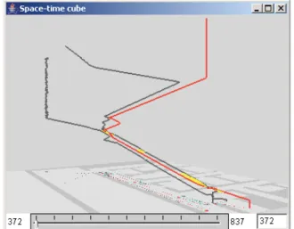
We shall not describe the further analysis in detail. In brief, we applied our computational tool for finding indications of probable interactions, i.e. cases of spatial proximity of moving agents. We found that only three of 23 people might have interactions with some of the victims or suspects. One of them was in the same room as Cecil Dennison (one of the suspects) till moment 262, when the latter left the room. The other two people might have interacted with Olive Palmer, a possible victim who stopped moving later than the other victims (Figure 8). In a case of a real investigation, it would be reasonable to interrogate these three persons.
Figure 8. Yellow marks the probable interactions between one of the possible casualties, whose trajectory is in red, and two
other people.
Hence, in the mini-challenge “Evacuation traces”, the density-based clustering of trajectories was useful for two purposes. First, we divided people into groups according to their fates. Two of the groups were interpreted as probable casualties, the others as survivors. Second, we separated normal movement behaviors from peculiar ones. Such separation is possible owing to the specific feature of the density-based clustering, which does not put an object in a cluster if it is not sufficiently similar to others. The flexibility of the clustering tool allows us to choose distance functions according to the goals of the analysis. As will be seen in the next section, the same clustering tool is applicable to a different type of data provided that a suitable distance function is used.
4.
MINI-CHALLENGE “MIGRANT
BOATS”
The dataset for this mini-challenge consists of 917 records about landings and interdictions of migrant boats with the spatial positions (geographical coordinates) and times of the landing or
interdiction events. The time span of the dataset is three years from the beginning of 2005 till the end of 2007. Among the questions of the mini-challenge, there are questions about the choice of the landing sites over the three years and about the geographic patterns of the interdictions over the three years. These questions may be answered with the help of clustering: using an appropriate distance function, we can discover spatio-temporal clusters of events, in particular, landings or interdictions in the same or close places shortly one after another.
4.1
Spatio-temporal clusters of landings
From the whole set of records, we select only the records about the landings. There are 441 such records. We apply the clustering tool with the distance function “spatio-temporal distance” described in Section 2. With 50 km as the spatial threshold and 21 days as the temporal threshold, we obtain the clusters shown in Figure 9 on a map and in a space-time cube (the use of space-time cube for visual exploration of event data is described in [4] and [7]). The scatterplot in Figure 10 aptly complements these two views. The horizontal and vertical dimensions of the plot represent the time and the latitude of the landings, respectively.
Figure 9. Spatio-temporal clusters of landings on a map (left) and in a space-time cube (right).
Figure 10. The clusters of landings shown on a scatterplot.
There are two big spatio-temporal clusters of landings located at the coast of Mexico. In the space-time cube, these two clusters appear as vertically aligned dots colored in orange and dark blue. In the scatterplot, the corresponding dots are aligned horizontally.
The temporal extent of the orange cluster, which consists of 39 landings, is from April 15 till September 22, 2006. The dark blue cluster consists of 146 landings, which occurred during the period from February 21 till November 18, 2007. Hence, both the number of landings at the Mexican coast and the duration of the period of active migration significantly increased from 2006 to 2007. As can be seen from the space-time cube and the scatterplot, there were no landings in this area before April 2006. The spatio-temporal clusters of landings at the coast of Florida and nearby islands are much smaller. In 2005, there were 3 clusters of landings, shown in blue, yellow, and red (5, 9, and 9 landings, respectively); all of them occurred on the islands of the Florida Keys archipelago. In 2006, there were 4 clusters of landings on the Florida Keys islands (light blue, violet, green, and dark red; 26 events in total) and 3 clusters of landings on the western coast of Florida (light cyan, pink, and dark yellow; 16 events in total). In 2007 there was only one spatio-temporal cluster consisting of 6 landings. It is shown in brown; the landings occurred on the western coast of Florida. This may mean that the migrants changed the strategy and avoided repeated landings in the same areas in favor of more distributed targets. This may also mean that repeated attempts to reach the same place were intercepted by the coast guards.
4.2
Spatial clusters of landings
Another kind of analysis can be done by means of spatial clustering of the landing events irrespective of the time. For this purpose, we apply the distance function “spatial distance”.
Figure 11. Left: spatial clusters of landings. Right: the distribution of the landings by years.
With the distance threshold 25km, we obtain the spatial clusters of landings demonstrated in Figure 11 left. The temporal histogram in Figure 11 right shows us how the destinations of the migrants changed over the three years. The bars of the histogram correspond to the years; they are divided into colored segments proportionally to the numbers of landings from the corresponding clusters. We can see that almost all landings in 2005 occurred on the Florida Keys archipelago (red cluster). In 2006, additional destinations appear: at the Mexican coast (orange), on the western coast of Florida (violet, light blue, and dark gray), and at the western end of Florida Keys (pink and yellow). In 2007, the number of landings on Florida Keys significantly decreases while the number of landings in Mexico dramatically increases. Besides, there is an eastern trend: many migrants land on the
eastern coast of Florida, which did not occur in the previous years.
4.3
Clustering of the interdictions
Now we shall apply clustering to the interdiction events. In Figure 12, we see the spatio-temporal clusters discovered with the use of the distance function “spatio-temporal distance” (maxD=50 km;
maxT=21 days). In Figure 13, we can see how the clusters and the remaining interdiction events (“noise”) are distributed over the three years from 2005 to 2007. The temporal histogram in Figure 14 left shows us the sizes of the clusters and “noise” by years.
Figure 12. Spatio-temporal clusters of interdictions on a map (left) and in a space-time cube (right).
Figure 13. Spatio-temporal clusters of interdictions by years.
Figure 14. Left: the sizes of the clusters of the interdictions and the “noise” by years. Right: the landings in Florida and
on nearby islands in the same years.
The spatio-temporal clusters of interdictions are generally larger than the spatio-temporal clusters of landings (Figure 9), except for the landings in Mexico. This refers not only to the number of events in a cluster but also to its spatial and temporal extent. The larger clusters mean that the interdiction events are spatially and temporally denser than the landing events. The highest spatio-temporal density of the interdictions is reached in 2006, when a
single cluster (violet) includes 103 out of 170 events, i.e. over 60%. Like in 2005, the events are concentrated in the area between Florida Keys and Isla Del Sueño, the origin of the migrant trips; however, the spatial extent is larger in 2006. In 2007, the spatial spreading of the interdictions further increases while the spatio-temporal density of the events decreases. This is signified by the larger number of smaller clusters; the largest cluster (light green) is smaller and looser than the largest clusters in the previous years. The ratio between the number of events in the clusters and the size of the “noise” (58 to 142) is much smaller in 2007 than in 2006 (103 to 67) and 2005 (58 to 48).
When we compare these observations with the observations concerning the landings (Sections 4.1 and 4.2), we can conclude that the strategy of the migrants changed over the three years: the migrants diversified their destinations and, evidently, the routes. This, apparently, made the coast guards extend the area of patrolling. Probably, the migrants hoped that the change of the strategy would make them harder to catch and thereby increase the success rate. If we compare the number of landings in Florida and on the nearby islands (visualized on a histogram in Figure 14 right) with the number of interdictions by years, we may conclude that the success rate, indeed, steadily increased over the three years. The ratio between the number of landings and the number of interdictions was 46:106 (0.43) in 2005, 88:170 (0.51) in 2006, and 116:200 (0.58) in 2007. In 2006 and 2007 there were also 41 and 150 landings and no interdictions in Mexico.
For the landing events, we used spatial clustering irrespective of the time, which produced meaningful spatial clusters (Section 4.2). However, this method of clustering does not work well for the interdictions: due to the high spatial density of the events, most of them are united in a single very large cluster. This does not give us new opportunities for the analysis.
Hence, in the mini-challenge “Migrant boats”, the density-based clustering helped us to detect compact groups of events in space and time, to asses the spatio-temporal density of the events and its change over time, and to divide events into groups according to their spatial positions in order to examine the changes in the spatial distribution of the events over time.
5.
CONCLUSION
Clustering in combination with interactive visual displays is a powerful instrument of data analysis, in particular, when the data are large and/or complex. Many clustering methods require the data to be represented as points in a multi-dimensional space of properties (in other terms, by feature vectors). However, for complex data with multiple heterogeneous properties there may be no adequate representation by feature vectors. An example of such a complex data type is trajectories of moving objects, characterized by the origin and destination, length, temporal extent, duration, geometrical shape, spatial orientation, dynamics (distribution of the speeds along the way), and, possibly, variation of other attributes during the movement.
A possible approach to the clustering of complex data types is the use of a generic clustering algorithm with a type-specific distance function, which properly accounts for the relevant properties depending on their nature. We have demonstrated this approach by applying the same clustering algorithm to two datasets of different types, trajectories of moving objects and point events
distributed in space and time. We have also demonstrated that different distance functions oriented to the same type of data may be useful for different analysis tasks.
The clustering tool we use implements a density-based clustering algorithm, which does not strive to put each object in some cluster but finds compact groups of close (similar) objects and leaves the other objects ungrouped. In this way, it not only discovers frequent patterns (combinations of properties) but also enables the analyst to examine the variation of the data density (in terms of close properties) throughout the dataset. In the paper, we have demonstrated how the features of the algorithm are exploited in the analysis.
The VAST Challenge datasets [8] we have used in this paper are quite small; they could be effectively analyzed without the use of clustering. For larger datasets, clustering gives more significant advantages. Our clustering-based visual analytics tools work well with about 5,000 trajectories, i.e. the reaction time is appropriate for an interactive analysis. Clustering of 10,000 trajectories is possible but requires some patience.
Currently we continue our research related to clustering in two major directions. First, we extend the approach to other types of spatio-temporal data, in particular, interactions between moving objects (mentioned in Section 3.2). In the future, we shall also extend it to spatially referenced time series data. Second, we look for ways to increase the scalability of clustering with respect to the size of the data. Thus, we have recently devised a visual analytics method for extracting clusters from a dataset not fitting in the computer main memory [1].
6.
ACKNOWLEDGMENTS
The work has been done partly within the EU-funded research project GeoPKDD – Geographic Privacy-aware Knowledge Discovery and Delivery (IST-6FP-014915; http://www.geopkdd.eu) and partly within the research project ViAMoD – Visual Spatiotemporal Pattern Analysis of Movement and Event Data, which is funded by DFG – Deutsche Forschungsgemeinschaft (German Research Foundation) within the Priority Research Programme “Scalable Visual Analytics” (SPP 1335).
The work on interactive cluster analysis of trajectories was done together with our GeoPKDD partners from the University of Pisa, Italy. We are grateful to them for the cooperation and specially thank Salvatore Rinzivillo for the implementation of the clustering algorithm OPTICS in the way allowing the use of different distance functions.
7.
REFERENCES
[1] Andrienko, G., Andrienko, N., Rinzivillo, S., Nanni, M., Pedreschi, D., Giannotti, F. 2009. Interactive Visual Clustering of Large Collections of Trajectories. VAST 2009
(submitted).
[2] Andrienko, G., Andrienko, N., and Wrobel, S. 2007. Visual Analytics Tools for Analysis of Movement Data. ACM SIGKDD Explorations, 9(2): 38-46.
[3] Andrienko, N., and Andrienko, G. 2008. Evacuation Trace Mini Challenge Award: Tool Integration. Analysis of
Movements with Geospatial Visual Analytics Toolkit. Proc. VAST 2008, IEEE Computer Society Press, 205-206.
[4] Andrienko, N., Andrienko, G., and Gatalsky, P. 2003. Exploratory Spatio-Temporal Visualization: an Analytical Review. Journal of Visual Languages and Computing, 14 (6), 503-541
[5] Ankerst, M., Breunig, M., Kriegel, H.-P., and Sander, J. 1999. OPTICS: Ordering points to identify the clustering structure. In Proc. ACM SIGMOD 1999, 49–60.
[6] Ester, M., Kriegel, H.-P., Sander, J., and Xu, X. 1996. A density-based algorithm for discovering clusters in large spatial databases with noise. In Proc. ACM KDD 1996, 226-231.
[7] Gatalsky, P., Andrienko, N., and Andrienko, G. 2004. Interactive Analysis of Event Data using Space-Time Cube. In Banissi, E. et al. (Eds.) Proc. IV 2004 - 8th International
Conference on Information Visualization, July 2004, London, UK, 145-152
[8] Grinstein, G, Plaisant, C., O’connell, T., Laskowski, S. Scholtz, J., Whiting, M. VAST 2008 Challenge: Introducing Mini-Challenges, Proceedings of IEEE Symposium on Visual Analytics Science and Technology (2008)
[9] Hägerstrand, T. 1970. What about people in regional science? In: Papers of the Regional Science Association, 24, 7-21.
[10] Kraak, M.-J. 2003. The space-time cube revisited from a geovisualization perspective, in: Proc. 21st International Cartographic Conference, Durban, South Africa, August 2003, 1988-1995.
[11] Rinzivillo, S., Pedreschi, D., Nanni, M., Giannotti, F., Andrienko, N., and Andrienko, G. 2008. Visually–driven analysis of movement data by progressive clustering,