This is a repository copy of Multinomial VaR Backtests : A simple implicit approach to backtesting expected shortfall.
White Rose Research Online URL for this paper: http://eprints.whiterose.ac.uk/126410/
Version: Accepted Version Article:
McNeil, Alexander John orcid.org/0000-0002-6137-2890, Kratz, Marie and Lok, Yen Hsiao (2018) Multinomial VaR Backtests : A simple implicit approach to backtesting expected shortfall. Journal of Banking and Finance. JBF-D-16-01251R1. ISSN 1872-6372
https://doi.org/10.1016/j.jbankfin.2018.01.002
Reuse
This article is distributed under the terms of the Creative Commons Attribution-NonCommercial-NoDerivs (CC BY-NC-ND) licence. This licence only allows you to download this work and share it with others as long as you credit the authors, but you can’t change the article in any way or use it commercially. More
information and the full terms of the licence here: https://creativecommons.org/licenses/ Takedown
If you consider content in White Rose Research Online to be in breach of UK law, please notify us by
Multinomial VaR Backtests:
A simple implicit approach to backtesting expected
shortfall
Marie Kratz
∗, Yen H. Lok
†, Alexander J. McNeil
‡Abstract
Under the Fundamental Review of the Trading Book, capital charges are based on the coherent Expected Shortfall (ES) risk measure, which is sensitive to tail risk. We argue that backtesting of the forecasting models used to derive ES can be based on a multinomial test of Value-at-Risk (VaR) exceptions at several levels. Using simulation experiments with heavy-tailed distributions and GARCH volatility models, we design a statistical procedure to show that at least four VaR levels are required to obtain tests for misspecified trading book models that are more powerful than single-level (or even two-level) binomial exception tests. A traffic-light system for model approval is pro-posed and illustrated with three real-data examples spanning the 2008 financial crisis.
JEL classification: C12; C52; D81; G18; G28; G32
∗ESSEC Business School, CREAR risk research center; E-mail: [email protected] †Heriot Watt University; E-mail: [email protected]
Keywords: Backtesting; Banking regulation; Expected Shortfall; Financial risk man-agement; Statistical test; Value-at-Risk
1 Introduction
Techniques for the measurement of risk are central to the process of managing risk in finan-cial institutions and beyond. In banking and insurance it is standard to model risk with probability distributions and express risk in terms of scalar-valued risk measures. Formally speaking, risk measures are mappings of random variables representing profits and losses (P&L) into real numbers representing capital amounts required as a buffer against insol-vency. The seminal work of Artzner et al. (1999) proposed a set of desirable mathematical properties defining a coherent risk measure, including the important axioms of subadditiv-ity, which requires that the benefits of diversification in a risky portfolio are respected, and positive homogeneity, which requires a linear scaling of the risk measure with portfolio size. The two main risk measures used in financial institutions and regulation are value-at-risk (VaR) and expected shortfall (ES), the latter also known as tail value-at-risk (TVaR) or conditional value-at-risk (CVaR). VaR is defined as a quantile of the P&L distribution and, despite the fact that it is not coherent, it has been the dominant risk measure in banking regulation. It is also the risk measure used in Solvency II insurance regulation in Europe, where the Solvency Capital Requirement (SCR) is defined to be the 99.5% VaR of an an-nual loss distribution. Expected shortfall at level α is the conditional expected loss given exceedance of VaR at that level and is a coherent risk measure (Acerbi and Tasche, 2002; Tasche, 2002). For this reason, and also because it is a more tail-sensitive measure of risk, it has attracted increasing regulatory attention in recent years. ES at the 99% level for annual losses is the primary risk measure of the Swiss Solvency Test (SST). As a result of the Fundamental Review of the Trading Book (Basel Committee on Banking Supervision, 2013) a 10-day ES at the 97.5% level will be the main measure of risk for setting trading
book capital under Basel III (Basel Committee on Banking Supervision, 2016).
For a given risk measure, the key practical challenge is to estimate it accurately using statistical models, and to validate estimates by checking whether realized losses, observed ex post, are in line with the ex ante estimates or forecasts. The statistical procedure by which we compare realizations with forecasts is known as backtesting.
The aim of this paper is to propose a simple approach to backtesting, which may be viewed in two ways. On the one hand, we suggest a natural extension to standard VaR backtesting that allows us to test VaR estimates at different probability levels; on the other hand, our approach can be viewed as providing an implicit backtest for ES.
Fundamental questions have been raised in the statistical forecasting literature about what it means to backtest a sequence of risk measure estimates or forecast models. Although ES appears to be a more suitable risk measure than VaR because of its coherence and tail sensitivity, it has been shown that, in contrast to VaR, it lacks the property of elic-itability (Gneiting, 2011). Since elicitable risk measures admit so-called consistent scoring functions for comparing competing forecasts of the risk measure, this has been interpreted as calling into question our ability to backtest ES estimates. However, ES has been shown to be conditionally elicitable (Emmer et al., 2015) and jointly elicitable with VaR (Fissler and Ziegel, 2016), and a number of papers demonstrate that it is certainly possible to devise backtests based on ES and VaR estimates that are are sensitive to systematic underestima-tion of ES, a primary concern of regulators (McNeil and Frey, 2000; Nolde and Ziegel, 2017; Acerbi and Szekely, 2017).
The literature on backtesting VaR estimates is large and based on the observation that when VaR at level α is accurately estimated, the VaR exceptions, that is the occasions on which realized losses exceed VaR forecasts, should form a sequence of independent,
identi-cally distributed Bernoulli variables with probability (1−α). The simple binomial test for the number of exceptions is often described as a test ofunconditional coverage, while a test that also explicitly examines the independence of exceptions is a test of conditional cover-age. Important contributions to VaR backtesting include Kupiec (1995), Dav´e and Stahl (1998), Christoffersen (1998), Christoffersen and Pelletier (2004) and the overview article of Berkowitz et al. (2011). Colletaz et al. (2013) consider the construction of a VaR backtest at two levels and introduce the concept of a risk map to account for both the number and magnitude of extreme losses (see also Wied (2016)) for multivariate backtests).
The literature on ES backtesting is smaller but rapidly increasing since the publication of the recommendations of FRTB. Tests may be categorized into those which make explicit reference to estimates of ES and VaR and those, like the ones proposed in the current study, which test ES estimates implicitly by testing aspects of the tail models from which they are directly derived. Among the explicit approaches are the test of McNeil and Frey (2000) based on violation residuals, the Monte Carlo hypothesis test of Acerbi and Szekely (2014) and the recent ridge backtest of Acerbi and Szekely (2017).
Most implicit tests can be viewed or represented as tests based on threshold exceedances by PIT (probability-integral-transform) values. PIT values are estimates of the probability of observing ex post losses up to a certain level according to the underlying forecast model; they should form an iid uniform sample when forecast models are consistent with ex post losses. Diebold et al. (1998, 1999) showed how PIT values can be used to evaluate the overall quality of density forecasts and Berkowitz (2001) proposed a test of forecast distributions in the tail based on the idea of truncating PIT values above a level α. Blum (2004) proposed a variety of extensions of PIT methodology to overlapping forecast intervals, multiple forecast horizons and the validation of ES estimates which have been used in some reinsurance companies for
more than a decade.
Implicit tests of ES that are effectively based on functions of PIT exceedances include the test of Kerkhof and Melenberg (2004), the Z-test proposed by Costanzino and Curran (2015), which applies to any so-called spectral risk measure, and the related test of Du and Escan-ciano (2017), based on the concept of a cumulative violation process; see also Costanzino and Curran (2016) where an implicit ES backtest is used to propose a traffic-light system analogous to the Basel system for VaR exceptions.
Although the FRTB has recommended that ES be adopted as the main risk measure for the trading book under Basel III (Basel Committee on Banking Supervision, 2016), it is notable that the backtesting regime will still largely be based on VaR exceptions at the 99% level, albeit also for individual trading desks as well as the whole trading book. The Basel publication does however state that banks will be required to go beyond the basic mandatory requirement to also consider more advanced backtests. A number of possibilities are listed including: tests based on VaR at multiple levels (97.5% and 99% are explicitly mentioned); tests based on both VaR and ES; tests based on PIT-values.
The idea of a multilevel VaR backtest serving as an implicit backtest of expected shortfall stems naturally from an approximation of ES proposed by Emmer et al. (2015). Denoting the ES and VaR of the distribution of the loss L by ESα(L) and VaRα(L), these authors show that
ESα(L) ≈ 1
4 [q(α) +q(0.75α+ 0.25) +q(0.5α+ 0.5) +q(0.25α+ 0.75) ] (1.1) where q(γ) =V aRγ(L). This suggests that an estimate of ESα(L) derived from a model for the distribution ofLcould be considered reliable if estimates of the four VaR valuesq(aα+b)
derived from the same model are reliable. It leads to the intuitive idea of backtesting ES via simultaneously backtesting multiple VaR estimates at different levels.
In this paper we propose multinomial backtests of VaR exceptions at multiple levels, exam-ining the properties of the tests and answering the following main questions:
Q1. Does a multinomial test work better than a binomial test for model validation? Q2. What type of multinomial test should be used?
Q3. What is the optimal number of quantiles that should be used in terms of size, power and stability of results, as well as simplicity of the procedure?
A guiding principle of our study is to provide a simple and reliable statistical test which is not much more complicated (conceptually and computationally) than the binomial test based on VaR exception counts that dominates industry and regulatory practice.
We require a test where size can be accurately controlled and where we can attain reasonable power to reject models that give poor estimates of the tail, which would lead to poor esti-mates of expected shortfall. Although we certainly aim to provide tests that are much more powerful than the binomial test, the maximization of power is not the overriding concern. Our proposed backtest might be beaten for power by other tests based on PIT values, but it gives impressive results nonetheless and we believe it is a much easier test to interpret for practitioners and regulators. It also leads to a very intuitive traffic-light system for model validation that extends and improves the existing Basel traffic-light system.
The structure of the paper is as follows. Sections 2 and 3 form the core material of the study. The multinomial backtest is defined in Section 2 and three variants are proposed: the stan-dard Pearson chi-squared test; the Nass test; a likelihood ratio test (LRT). Section 3 contains a large Monte Carlo simulation study in several parts to demonstrate the performance of the
tests in different situations.
In Section 4 we give our views on the best design for the backtest. We also show how a traffic-light system may be designed. In Section 5, we apply our approach to real data, considering in turn: an investment in the S&P index; a portfolio subject to equity and FX risk; and, finally, a long position in a European call option. Conclusions are found in Section 6.
2 Multinomial tests
2.1 Testing set-up
Suppose we have a series of ex-ante predictive models {Ft, t = 1, . . . , n} and a series of ex-post losses {Lt, t = 1, . . . , n}. At each time t the model Ft is used to produce estimates (or forecasts) of value-at-risk VaRα,t and expected shortfall ESα,t at various probability levelsα. The VaR estimates are compared withLt to assess the adequacy of the models in describing the losses, with particular emphasis on the most extreme losses.
In view of the representation (1.1), we consider the idea proposed in Emmer et al. (2015) of backtesting expected shortfall indirectly by simultaneously backtesting a number of VaR estimates at different levels α1, . . . , αN. We investigate different choices of the number of levels N in the simulation study in Section 3.
We generalize the idea of (1.1) by considering VaR probability levels α1, . . . , αN defined by
αj =α+
j−1
N (1−α), j = 1, . . . , N, N ∈N, (2.1)
for some starting levelα. In this paper we generally setα= 0.975 corresponding to the level used for expected shortfall calculation and the lower of the two levels used for backtesting
under the Basel rules for banks (Basel Committee on Banking Supervision, 2016); we will also consider α= 0.99 in the case whenN = 1 since this is the usual level for binomial tests of VaR exceptions. To complete the description of levels, we set α0 = 0 andαN+1 = 1.
We define the violation or exception indicator of the levelαj at timetby It,j :=I{Lt>VaRαj ,t}, where IA denotes an event indicator for the eventA.
It is well known (Christoffersen, 1998) that if the losses Lt have conditional distribution functions Ft then, for fixed j, the sequence (It,j)t=1,...,n should satisfy:
• the unconditional coverage hypothesis, E (It,j) = 1−αj for all t, and
• the independence hypothesis, It,j is independent of Is,j for s6=t.
If both are satisfied, the VaR forecasts at levelαj are said to satisfy the hypothesis of correct
conditional coverage and the number of exceptionsPn
t=1It,j has a binomial distribution with
success (exception) probability 1−αj.
Testing simultaneously VaR estimates at N levels leads to a multinomial distribution. If we define Xt = PNj=1It,j, then the sequence (Xt)t=1,...,n counts the number of VaR levels that
are breached. The sequence (Xt) should satisfy the two conditions:
• the unconditional coverage hypothesis, P (Xt ≤j) =αj+1, j = 0, . . . , N for all t,
• the independence hypothesis, Xt is independent of Xs fors 6=t.
Let MN(n,(p0, . . . , pN)) denotes the multinomial distribution with n trials, each of which may result in one of N+ 1 outcomes{0,1, . . . , N}according to probabilities p0, . . . , pN that sum to one. If we define observed cell counts by
Oj = n X
t=1
then, under the unconditional coverage and independence assumptions, the random vector (O0, . . . , ON) should follow the multinomial distribution
(O0, . . . , ON)∼MN(n,(α1−α0, . . . , αN+1−αN)) .
More formally, let 0 = θ0 < θ1 < · · · < θN < θN+1 = 1 be an arbitrary sequence of
parameters and consider the model
(O0, . . . , ON)∼MN(n,(θ1−θ0, . . . , θN+1−θN)) . (2.2) We test null and alternative hypotheses given by
H0 : θj =αj forj = 1, . . . , N
H1 : θj 6=αj for at least onej ∈ {1, . . . , N}.
(2.3)
2.2 Choice of tests
Various test statistics can be used to evaluate these hypotheses. Cai and Krishnamoorthy (2006) provide a relevant numerical study of the properties of five possible tests of multino-mial proportions. Here we propose to use three of them: the standard Pearson chi-square test; the Nass test, which performs better with small cell counts; the likelihood ratio test (LRT). More details are as follows.
1. Pearson chi-squared test (Pearson, 1900). The test statistic in this case is
SN = N X j=0 (Oj+1−n(αj+1−αj))2 n(αj+1−αj) d ∼ H0 χ 2 N, (2.4)
and a size κ test is obtained by rejecting the null hypothesis when SN > χ2N(1−κ), where χ2
N(1−κ) is the (1−κ)-quantile of the χ
2
N-distribution. It is well known that the accuracy of this test increases as min
0≤j≤Nn(αj+1−αj) increases and decreases with increasing N.
2. Nass test(Nass, 1959).
Nass introduced an improved approximation to the distribution of the statistic SN defined in (2.4), namely c SN d ∼ H0 χ 2 ν, with c= 2 E (SN) var(SN) and ν =cE (SN),
where E (SN) = N and var(SN) = 2N−
N2+ 4N + 1 n + 1 n N X j=0 1 αj+1−αj .
The null hypothesis is rejected when c SN > χ2ν(1−κ), using the same notation as before. The Nass test offers an appreciable improvement over the chi-square test when cell probabilities are small.
3. LRT(see, for example, Casella and Berger (2002) or Cai and Krishnamoorthy (2006)). Let L(p0, . . . , pN | O0, . . . , ON) denote the likelihood of the multinomial distribution (O0, . . . , ON) ∼ MN(n,(p0, . . . , pN)). The Maximum Likelihood Estimators (MLEs) of the parameters pj are given by ˆpj = Oj/n and the Likelihood-Ratio Test (LRT) statistic of the null and alternative hypotheses in (2.3) is
˜ SN =−2 ln L(α1−α0, . . . , αN+1−αN |O0, . . . , ON) L(ˆp0, . . . ,pˆN |O0, . . . , ON) = 2 X j:0≤j≤N,Oj6=0 Ojln Oj n(αj+1−αj) d ∼ H0 χ 2 N. (2.5)
The null hypothesis is rejected when ˜SN > χ2N(1−κ).
Note that it is also possible to construct variants on the multinomial LRT by embedding the null hypothesis in a parametric family of models as shown in Kratz et al. (2016b); the resulting tests can be more effective for largeN (above 16) but have a very similar performance for the values of N that interest us (up to 8) and lack the simplicity of the basic test described above.
2.3 The case N = 1
It may be easily verified that, for N = 1, the Pearson multinomial test statistic S1 in (2.4)
is the square of the binomial score test statistic
Z := n −1Pn t=1It,1−(1−α) p n−1α(1−α) = O1 −n(1−α) p nα(1−α) , (2.6) which is compared with a standard normal distribution; thus a two-sided score test gives identical results to the Pearson chi-squared test. In the case N = 1, the LRT described by (2.5) is the two-sided binomial test of unconditional coverage as described in Kupiec (1995) and Christoffersen (1998). In addition to the score test and LRT, we also consider a Wald test in which theαparameter in the denominator of (2.6) is replaced by the estimator ˆ θ1 =n−1 n X t=1 (1−It,1) = 1−O1/n.
In the case where N = 1, we also carry out one-sided variants of the LRT, score and Wald tests which test H0 : θ1 ≥ α against the alternative H1 : θ1 < α (underestimation of
VaR). One-sided score and Wald tests are straightforward to carry out, being based on the asymptotic normality of Z. To derive a one-sided LRT, it may be noted that the likelihood ratio statistic for testing the simple null hypothesis θ1 = α against the simple alternative
that θ1 =α∗ with α∗ < α depends on the data through the the number of VaR exceptions
B =Pn
t=1It,1. In the one-sided LRT, we test B against a binomial distribution; this test at
the 99% level is the one that underlies the Basel backtesting regime and traffic light system.
3 Simulation studies
To answer our main questions (Q1 to Q3 in Section 1), we conduct a series of experiments based on simulated data. In Section 3.1 we carry out a comparison of the size and power of our tests. The power experiments consider misspecifications of the loss distribution using distributional forms that might be typical for the trading book; we are particularly interested to see whether the multinomial tests can distinguish more effectively than binomial tests between distributions with different tails.
In Sections 3.2 and 3.3, we carry out backtesting experiments in which we look at the ability of the tests to distinguish between the performance of different modellers who estimate quantiles with different methodologies and are subject to statistical error. The backtests of Section 3.2 take a static distributional view; in other words, the true data generating process is simply a distribution as in the size-power comparisons of Section 3.1.
In Section 3.3 we take a dynamic view and consider a data-generating process that features a GARCH model of stochastic volatility with heavy-tailed innovations. We consider the ability of the multinomial tests to distinguish between good and bad forecasters, where the latter may misspecify the form of the dynamics and/or the conditional distribution of the losses.
3.1 Size and Power
3.1.1 Theory
To judge the effectiveness of the three multinomial tests (and the additional binomial tests), we compute their size γ = P (reject H0|H0 true) (type I error) and power 1 − β = 1 −
P (accept H0|H0 false) (1- type II error). For a given size, regulators should clearly be interested in having more powerful tests for exposing banks working with deficient models. Checking the size of the multinomial test requires us to simulate data from a multinomial distribution under the null hypothesis (H0). This can be done indirectly by simulating data from any continuous distribution (such as normal) and counting the observations between the true values of the αj-quantiles.
To calculate the power, we have to simulate data from multinomial models under the alter-native hypothesis (H1). We choose to simulate from models with parameters given by
θj =G(F←(αj))
where F and G are distribution functions, F←(u) = inf{x : F(x) ≥ u} denotes the
gener-alized inverse of F, and F and G are chosen such that θj 6=αj for one or more values of j.
G can be thought of as the true distribution and F as the model. If a forecaster usesF to determine theαj-quantile, then the true probability associated with the quantile estimate is
θj rather thanαj. We consider the case where F and G are two different distributions with mean zero and variance one, but different shapes.
In a time-series context we could think of the following situation. Suppose that the losses (Lt) form a time series adapted to a filtration (Ft) and that, for all t, the true
condi-tional distribution of Lt given Ft−1 is given by Gt(x) = G((x−µt)/σt) where µt and σt are Ft−1-measurable variables representing the conditional mean and standard deviation of
Lt. However a modeller uses the model Ft(x) = F((x−µt)/σt) in which the distributional form is misspecified but the conditional mean and standard deviation are correct. He thus delivers VaR estimates given by VaRα,t =µt+σtF←(αj). The true probabilities associated with these VaR estimates areθj =Gt(VaRαj,t) = G(F
←(α
j))6=αj. We are interested in dis-covering whether the tests have the power to detect that the forecaster has used the models
{Ft, t= 1, . . . , n} rather than the true distributions{Gt, t= 1, . . . , n}.
Suppose for instance thatGis a Student t-distribution (scaled to have unit variance) andF
is a normal one, so that the forecaster underestimates the more extreme quantiles. In such a case, we will tend to observe too many exceedances of the higher quantiles.
The size calculation corresponds to the situation whereF =G; we calculate quantiles using the true model and there is no misspecification. In the power calculation, we focus on distri-butional forms for G that are typical for the trading book, having heavy tails and possibly skewness. We consider Student distributions with 5 and 3 degrees of freedom (t5 and t3), which have moderately heavy and heavy tails respectively, and the skewed Student distri-bution of Fern´andez and Steel (1998) with 3 degrees of freedom and a skewness parameter
γ = 1.2 (denoted st3); in all cases we take the benchmark model F to be standard normal. Table 1 provides motivation for the need to consider at least 2 quantiles in an implicit backtest of ES. It shows the values of VaR0.975, VaR0.99 and ES0.975 for the four distributions
used in the simulation study which have all been calibrated to have mean zero and variance one. Note how the value of ES0.975 gets progressively larger as we move down the table;
the final column marked ∆2 shows the percentage increase in the value of ES0.975 when
measure, it is particularly important that a bank can estimate this measure reliably. From a regulatory perspective it is important that backtesting procedure can distinguish the heavier-tailed models from the light-heavier-tailed normal distribution, since a modeller using the normal distribution would seriously underestimate ES0.975 if any of the other three distributions were
“the true distribution”. We observe that the three distributions give comparable values for VaR0.975; the t3 model actually gives the smallest value for this risk measure. The values
of VaR0.99 are ordered in the same way as those of ES0.975. The quantity ∆1, which gives
the percentage increase in the value of VaR0.99when compared with the normal distribution,
does not increase quite so dramatically as ∆2, which suggests that more than two quantiles
are required to implicitly backtest ES.
VaR0.975 VaR0.99 ∆1 ES0.975 ∆2
Normal 1.96 2.33 0.00 2.34 0.00 t5 1.99 2.61 12.04 2.73 16.68 t3 1.84 2.62 12.69 2.91 24.46 st3 (γ = 1.2) 2.04 2.99 28.68 3.35 43.11 Table 1: Values of VaR0
.975,VaR0.99 andES0.975 for four distributions used in simulation study (Normal, Student t5, Student t3, skewed Student t3 with skewness parameter γ= 1.2). Column∆1, ∆2 respectively, shows percentage increase inVaR0.99,ES0.975 respectively, compared with normal distribution.
To determine the VaR level values, we set N = 2k for k = 0,1,· · · ,6. In all multinomial experiments with N ≥2, we set α1 =α= 0.975 and further levels are determined by (2.1).
We choose sample sizes n1 = 250,500,1000,2000 and estimate the rejection probability for
the null hypothesis using 10,000 replications.
In the case N = 1, we consider a series of additional binomial tests of the number of exceptions of the level α1 = α and present these in a separate table; in this case we also
consider the level α = 0.99, as in current practice, in addition to α = 0.975. This gives us the ability to compare our multinomial tests with all binomial test variants at both levels.
α 0.975 0.990
twosided TRUE FALSE TRUE FALSE
G n |test Wald score LRT Wald score LRT Wald score LRT Wald score LRT
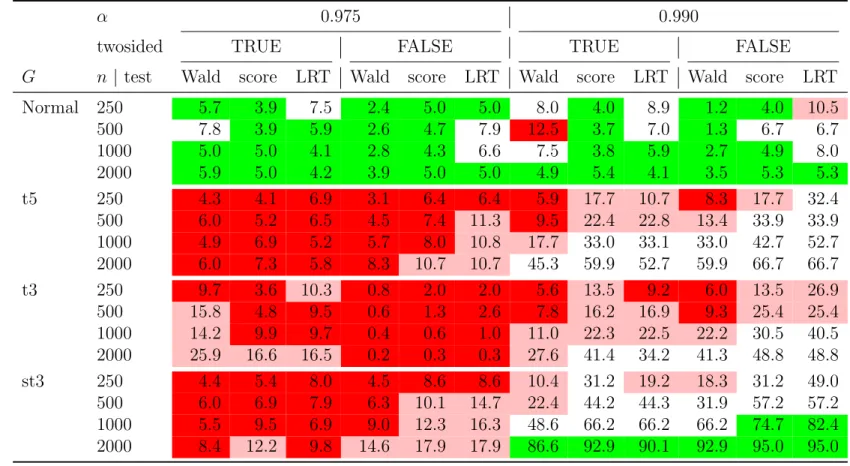
Normal 250 5.7 3.9 7.5 2.4 5.0 5.0 8.0 4.0 8.9 1.2 4.0 10.5 500 7.8 3.9 5.9 2.6 4.7 7.9 12.5 3.7 7.0 1.3 6.7 6.7 1000 5.0 5.0 4.1 2.8 4.3 6.6 7.5 3.8 5.9 2.7 4.9 8.0 2000 5.9 5.0 4.2 3.9 5.0 5.0 4.9 5.4 4.1 3.5 5.3 5.3 t5 250 4.3 4.1 6.9 3.1 6.4 6.4 5.9 17.7 10.7 8.3 17.7 32.4 500 6.0 5.2 6.5 4.5 7.4 11.3 9.5 22.4 22.8 13.4 33.9 33.9 1000 4.9 6.9 5.2 5.7 8.0 10.8 17.7 33.0 33.1 33.0 42.7 52.7 2000 6.0 7.3 5.8 8.3 10.7 10.7 45.3 59.9 52.7 59.9 66.7 66.7 t3 250 9.7 3.6 10.3 0.8 2.0 2.0 5.6 13.5 9.2 6.0 13.5 26.9 500 15.8 4.8 9.5 0.6 1.3 2.6 7.8 16.2 16.9 9.3 25.4 25.4 1000 14.2 9.9 9.7 0.4 0.6 1.0 11.0 22.3 22.5 22.2 30.5 40.5 2000 25.9 16.6 16.5 0.2 0.3 0.3 27.6 41.4 34.2 41.3 48.8 48.8 st3 250 4.4 5.4 8.0 4.5 8.6 8.6 10.4 31.2 19.2 18.3 31.2 49.0 500 6.0 6.9 7.9 6.3 10.1 14.7 22.4 44.2 44.3 31.9 57.2 57.2 1000 5.5 9.5 6.9 9.0 12.3 16.3 48.6 66.2 66.2 66.2 74.7 82.4 2000 8.4 12.2 9.8 14.6 17.9 17.9 86.6 92.9 90.1 92.9 95.0 95.0
Table 2: Estimated size and power of three different types of binomial test (Wald, score, likelihood-ratio test (LRT)) applied to exceptions of the 97.5% and 99% VaR estimates. Both one-sided and two-sided tests have been carried out. Results are based on 10,000 replications. Green indicates good results (≤ 6% for the size; ≥ 70% for the power); red indicates poor results (≥9% for the size; ≤30% for the power); dark red indicates very poor results (≥12% for the size; ≤10% for the power).
3.1.2 Binomial test results
Table 2 shows the results for one-sided and two-sided binomial tests for the number of VaR exceptions at the 97.5% and 99% levels. In this table and in Table 3, the following color coding is used: green indicates good results (≤6% for the size; ≥ 70% for the power); red indicates poor results (≥9% for the size;≤30% for the power); dark red indicates very poor results (≥12% for the size; ≤10% for the power).
97.5% level. The size of the tests is generally reasonable. The score test in particular always seems to have a good size for all the different sample sizes in both the one-sided and two-sided tests. The power of all the tests is extremely weak, which reflects the fact that the 97.5% VaR values in all of the distributions are quite similar. Note that the one-sided tests are slightly more powerful at detecting the t5 and skewed t3 models whereas two-sided tests are slightly better at detecting the t3 model; the latter observation is due to the fact that the 97.5% quantile of a (scaled) t3 is actually smaller than that of a normal distribution; see Table 1.
99% level. At this level the size is more variable and often too high in the smaller samples; in particular, the one-sided LRT (the Basel exception test) has a poor size in the case of the smallest sample. Once again the score test seems to have the best size properties.
The tests are more powerful in this case because there are more pronounced differences between the quantiles of the four models. One-sided tests are somewhat more powerful than two-sided tests since the non-normal models yield too many exceptions in comparison with the normal. The score test and LRT seem to be a little more powerful than the Wald test. We only get high power (green cells) in the case of the largest samples (1000 and 2000) from
the distribution with the longest right tail (skewed t3).
3.1.3 Multinomial test results
The results are shown in Table 3 and displayed graphically in Figure 1. Note that, as discussed in Section 2.3, the Pearson test with N = 1 gives identical results to the two-sided score test in Table 2. In the case N = 1, the Nass statistic is very close to the value of the Pearson statistic and also gives much the same results. The LRT with N = 1 is the two-sided LRT from Table 2.
Size of the tests. The results for the size of the three tests are summarized in the first panel of Table 3 whereG is Normal and in the first row of pictures in Figure 1.
The size of the Pearson χ2
-test deteriorates rapidly for N ≥8 showing that this test is very sensitive to bin size. The Nass test has the best size properties being very stable for all choices of N and all sample sizes. In contrast to the other tests, the size is always less than or equal to 5% for 2 ≤ N ≤ 8; there is a slight tendency for the size to increase above 5% whenN exceeds 8. The LRT has quite an unstable size, especially when compared with the Nass test; it tends to offer better results for a sample size n≥1000 and N ≤4.
Power of the tests. The results for the power of the three tests are summarized in panels 2–4 of Table 3 for different true underlying distributions G. In rows 2–4 of Figure 1 the power of the three tests is shown graphically as a function of N.
A first important observation is the sensitivity of power to the choice ofN; in generalN ≥4 is needed to attain reasonable power. The binomial test (N = 1) exhibits almost no power (the corresponding columns are all red) and the case N = 2 has poor power (the corresponding
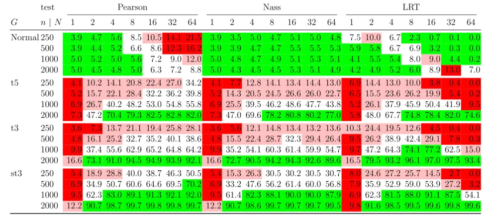
test Pearson Nass LRT G n | N 1 2 4 8 16 32 64 1 2 4 8 16 32 64 1 2 4 8 16 32 64 Normal 250 3.9 4.7 5.6 8.5 10.5 14.1 21.5 3.9 3.5 5.0 4.7 5.1 5.0 4.8 7.5 10.0 6.7 2.3 0.7 0.1 0.0 500 3.9 4.4 5.2 6.6 8.6 12.3 16.2 3.9 3.9 4.7 4.7 5.5 5.5 5.3 5.9 5.8 6.7 6.9 3.2 0.3 0.0 1000 5.0 5.2 5.0 5.6 7.2 9.0 12.0 5.0 4.8 4.7 4.9 5.1 5.3 5.1 4.1 5.5 5.4 8.0 9.0 4.4 0.2 2000 5.0 4.5 4.8 5.0 6.3 7.2 8.8 5.0 4.3 4.5 4.5 5.3 5.1 4.9 4.2 4.9 5.2 6.0 8.9 13.0 7.0 t5 250 4.1 10.2 14.1 20.8 22.4 27.0 34.2 4.1 7.7 12.8 14.1 13.4 14.4 13.0 6.9 14.4 13.0 10.0 3.8 0.4 0.0 500 5.2 15.7 22.1 28.4 32.2 36.2 39.8 5.2 14.3 20.5 24.5 26.6 26.0 22.7 6.5 15.5 23.6 26.2 19.9 5.4 0.2 1000 6.9 26.7 40.2 48.2 53.0 54.8 55.8 6.9 25.5 39.5 46.2 48.6 47.7 43.8 5.2 26.1 37.9 45.9 50.4 41.9 9.5 2000 7.3 47.2 70.4 79.3 82.5 82.8 82.0 7.3 47.0 69.6 78.2 80.8 80.2 77.0 5.8 48.0 67.7 74.8 78.4 82.0 74.6 t3 250 3.6 7.3 13.7 21.1 19.4 25.8 28.1 3.6 5.6 12.1 14.8 13.4 13.2 13.6 10.3 24.4 19.5 12.6 4.5 0.4 0.0 500 4.8 16.1 25.2 32.7 35.2 40.1 38.6 4.8 15.5 22.4 28.7 32.3 29.4 26.4 9.5 26.2 38.9 42.4 29.1 7.8 0.3 1000 9.9 37.4 55.6 62.9 65.2 64.8 64.2 9.9 35.2 54.1 60.3 61.4 59.9 54.7 9.7 47.2 64.3 74.1 77.2 62.5 15.0 2000 16.6 73.1 91.0 94.5 94.9 93.9 92.1 16.6 72.7 90.5 94.2 94.3 92.6 89.6 16.5 79.5 93.2 96.1 97.0 97.5 93.4 st3 250 5.4 18.9 28.8 40.0 38.7 46.3 50.5 5.4 15.3 26.3 30.5 30.2 30.5 30.7 8.0 24.6 27.2 25.7 14.5 2.7 0.0 500 6.9 34.9 50.7 60.6 64.6 69.5 70.2 6.9 33.2 47.6 56.2 61.4 60.0 56.8 7.9 35.9 52.9 59.0 53.9 27.2 3.2 1000 9.5 62.3 83.0 89.1 91.3 92.1 92.0 9.5 61.4 82.3 88.1 90.0 90.0 87.9 6.9 62.3 81.5 88.0 91.1 87.5 54.1 2000 12.2 90.7 98.7 99.7 99.8 99.8 99.7 12.2 90.7 98.6 99.7 99.7 99.7 99.5 9.8 91.6 98.5 99.5 99.6 99.8 99.6
Table 3: Estimated size and power of three different types of multinomial test (Pearson, Nass, likelihood-ratio test (LRT)) based on exceptions ofN levels. Results are based on 10,000 replications. Green indicates good results (≤6% for the size;
≥70% for the power); red indicates poor results (≥9% for the size; ≤30% for the power); dark red indicates very poor results (≥12% for the size; ≤10% for the power).
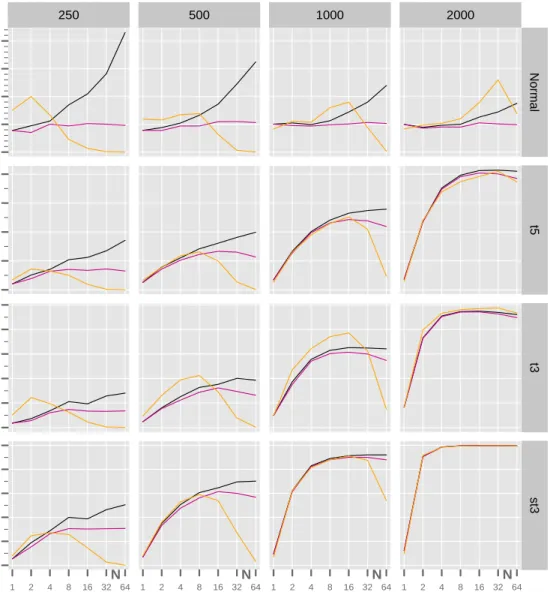
columns are never green, except for a sample size of 2000 and very heavy tails). There are large jumps in power betweenN = 1, N = 2 andN = 4, with the second jump being slightly smaller than the first. The general pattern observed in Figure 1 is an increase in power with
N (at first sharp, then moderate), then a relative stabilization for the Pearson test, a small decrease for the Nass test and a drop for the LRT (except when n= 2000).
The maximum power attained increases with the heaviness of the tail, as expected. Moreover the power of the three tests is broadly comparable for moderateN and the degree of similarity between the curves increases with sample size.
The power of the Nass test is generally slightly lower than that of the Pearson test; it tends to reach a maximum for N = 8 or N = 16 and then fall away - this would appear to be the price that is paid for the size-correction of the Pearson test which the Nass test undertakes. However, it is usually preferable to use a Nass test with N = 8 rather than a Pearson test with N = 4.
The LRT is not reliable when N exceeds 16, except for the largest sample size (2000). This is due to the presence of many cells with zero cell counts. The parametric version of the LRT proposed in Kratz et al. (2016a,b) can address this issue, but we prefer to retain simplicity by restrictingN to values less than 16.
To obtain a high power above 70% (green coloring), we generally need to take a sample size of 2000 in the case of t5 or t3; for the former we need at least N ≥ 4 levels and for the latter N ≥ 2 is sufficient. A sample size of n = 1000 suffices for the skewed t3 example provided that N ≥4 . These observations make sense since the degree of challenge for the tests decreases as we move down the table and the right tails of the distributions increase in weight.
Figure 1: Size (first row) and power of the three multinomial tests as a function ofN. The columns correspond to different sample sizes n and the rows to the different underlying distributionsG.
0 5 10 15 20 250 500 1000 2000 N o rm a l 0 20 40 60 80 t5 0 20 40 60 80 100 t3 1 2 4 8 16 32 64 N 0 20 40 60 80 100 1 2 4 8 16 32 64 N 1 2 4 8 16 32 64 N 1 2 4 8 16 32 64 N st 3 siz e/po w er
Summary. In general the Nass test with N = 4 or 8 appears to be a good compromise between a suitable size and power, and slightly preferable to the Pearson test or LRT with
N = 8, because of its more stable size property.
It seems clear that, regardless of the chosen test, we should pick N = 4 or 8, since the resulting tests are much more powerful than a binomial test or a joint test at only two VaR levels. In the remainder of the paper we will vary N only up to 8. Results for values from
N = 16 toN = 64 are available in Kratz et al. (2016b).
In Table 4, we collect the results for the multinomial tests with N = 4 levels (denoted P4, N4 and L4) and N = 8 levels (denoted P8, N8 and L8). We compare them with results for the two-sided binomial score test at the 99% level (i.e. the most powerful binomial test in Table 2), denoted B99, and for two examples of simple backtests that have been proposed for ES. These are the spectral backtest of Costanzino and Curran (2015) (denoted CC), which is very similar to the test of Du and Escanciano (2017), and a version of the test of McNeil and Frey (2000) (denoted MF) in which exceedance residuals are tested for mean-zero behavior with a t-test.
The superior performance of the multinomial tests to the three other tests (B99, CC and MF) is clearly apparent in terms of both size and power. The CC test does not work particularly well in our experiment and gives very similar results to the B99 test. The MF test generally has lower power than the multinomial tests for n ≤ 500 and only becomes competitive for
n≥1000; however, it has very power size.
Finally, it should be noted that the results of binomial tests are very sensitive to the choice of α. We have seen in Table 2 and Table 3 that their performance for α = 0.975 is very poor. The multinomial tests using a range of thresholds are much less sensitive to the exact choice of these thresholds, which makes them a more reliable type of test.
G n |test B99 P4 N4 LR4 P8 N8 LR8 CC MF Normal 250 4.0 5.6 5.0 6.7 8.5 4.7 2.3 4.5 9.1 500 3.7 5.2 4.7 6.7 6.6 4.7 6.9 4.6 8.2 1000 3.8 5.0 4.7 5.4 5.6 4.9 8.0 5.2 6.8 2000 5.4 4.8 4.5 5.2 5.0 4.5 6.0 4.8 5.6 t5 250 17.7 14.1 12.8 13.0 20.8 14.1 10.0 16.2 6.6 500 22.4 22.1 20.5 23.6 28.4 24.5 26.2 21.4 20.2 1000 33.0 40.2 39.5 37.9 48.2 46.2 45.9 30.8 55.9 2000 59.9 70.4 69.6 67.7 79.3 78.2 74.8 49.3 93.0 t3 250 13.5 13.7 12.1 19.5 21.1 14.8 12.6 11.5 7.7 500 16.2 25.2 22.4 38.9 32.7 28.7 42.4 13.1 25.9 1000 22.3 55.6 54.1 64.3 62.9 60.3 74.1 16.6 67.8 2000 41.4 91.0 90.5 93.2 94.5 94.2 96.1 22.4 95.6 st3 250 31.2 28.8 26.3 27.2 40.0 30.5 25.7 27.8 14.2 500 44.2 50.7 47.6 52.9 60.6 56.2 59.0 40.6 46.2 1000 66.2 83.0 82.3 81.5 89.1 88.1 88.0 61.7 87.1 2000 92.9 98.7 98.6 98.5 99.7 99.7 99.5 85.8 98.5 Table 4: Comparison of estimated size and power of the two-sided binomial score test (B99) with α= 0.99, the test of Costanzino and Curran (2015) (CC), a version of the test of McNeil and Frey (2000) (MF), and the multinomial tests, Pearson (P), Nass (N) and Likelihood-Ratio (LR), with N = 4 and 8. Results are based on 10,000 replications. The coloring scheme is the same as in Table 3.
3.2 Static backtesting experiment
The style of backtest we implement (both here and in Section 3.3) is designed to mimic the procedure used in practice where models are continually updated to use the latest market data. We assume that the estimated model is updated every 10 steps; if these steps are interpreted as trading days, this would correspond to every two trading weeks.
3.2.1 Experimental design
In each experiment we generate a total dataset ofn+n2 values from the true distributionG;
we use the same four choices as in the previous section. The lengthn of the backtest is fixed at the value 1000. The modeller uses a rolling window of n2 values to obtain an estimated
distribution F;n2 takes the values 250 and 500. We consider four possibilities for F:
The oracle who knows the correct distribution and its exact parameter values;
The good modeller who estimates the correct type of distribution (normal when G is normal, Student t when Gis t5 or t3, skewed Student when G is st3);
The poor modeller who always estimates a normal distribution (which is satisfactory only when Gis normal);
The industry modeller who uses the empirical distribution function by forming standard empirical quantile estimates, a method known as historical simulation in industry. To make the rolling estimation procedure clear, the modellers begin by using the data
L1, . . . , Ln2 to form their model F and make quantile estimates VaRαj,n2+1 forj = 1, . . . , N. These are then compared with the true losses {Ln2+i, i = 1, . . . ,10} and the exceptions of each VaR level are counted. The modellers then roll the dataset forward 10 steps and use the data L11, . . . , Ln2+10 to make quantile estimates VaRαj,n2+11 which are compared with
the losses {Ln2+10+i, i = 1, . . . ,10}; in total the models are thus re-estimated n/10 = 100 times.
We consider the same three multinomial tests as before and the same numbers of levels N. The experiment is repeated 1000 times to determine rejection rates.
3.2.2 Judging the quality of the modellers
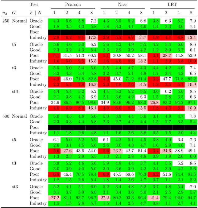
In Table 5 and again in Table 6 we use the same coloring scheme as previously, but a word of explanation is now required concerning the concepts of size and power.
The backtesting results for the oracle, who knows the correct model, should clearly be judged in terms of size since we need to control the type I error of falsely rejecting the null hypothesis that the oracle’s quantile “estimates” are accurate. We judge the results for the good modeller according to the same standards as the oracle. In doing this, we make the judgement that a sample of size n2 = 250 or n2 = 500 is sufficient to estimate quantiles
parametrically in a static situation when a modeller chooses the right class of distribution. We would not want to have a high rejection rate that penalizes the good modeller too often in this situation. Thus we apply the size coloring scheme to both the oracle and the good modeller.
The backtesting results for the poor modeller should clearly be judged in terms of power. We want to obtain a high rejection rate for this modeller who is using the wrong distribution, regardless of how much data he is using. Hence the power coloring is applied in this case. For the industry modeller the situation is more subtle. Empirical quantile estimation is an acceptable method provided that enough data is used. However it is less easy to say what is enough data because this depends on how heavy the tails of the underlying distribution
Test Pearson Nass LRT n2 G F |N 1 2 4 8 1 2 4 8 1 2 4 8 250 Normal Oracle 4.3 5.6 5.8 7.2 4.3 5.5 5.2 6.8 3.8 6.3 5.2 7.9 Good 1.8 3.5 4.3 5.8 1.8 3.3 4.1 4.6 1.4 3.3 3.6 7.1 Poor NA NA NA NA NA NA NA NA NA NA NA NA Industry 2.9 6.2 9.1 17.3 2.9 5.5 8.7 15.7 1.9 4.1 6.8 12.4 t5 Oracle 5.6 4.6 5.0 6.2 5.6 4.2 4.9 5.5 4.2 5.4 6.0 8.6 Good 2.3 3.2 4.3 5.4 2.3 2.9 3.9 4.2 1.2 3.0 3.7 6.1 Poor 5.1 31.5 51.3 60.2 5.1 30.8 50.2 58.1 3.1 28.7 44.8 52.9 Industry 1.6 5.0 9.5 15.5 1.6 4.6 8.8 13.2 1.1 3.9 5.8 10.0 t3 Oracle 5.5 5.0 5.4 5.0 5.5 4.4 4.7 4.3 4.4 4.2 4.6 7.4 Good 3.2 4.3 5.4 5.8 3.2 3.7 5.1 4.9 1.7 3.4 4.3 6.5 Poor 4.3 46.0 71.8 82.8 4.3 45.0 71.2 81.4 3.3 47.7 71.8 82.2 Industry 2.3 5.4 7.9 16.3 2.3 4.8 7.6 14.5 1.3 3.5 5.7 10.9 st3 Oracle 4.4 5.4 5.2 6.2 4.4 5.3 5.2 5.5 3.6 6.2 5.6 8.5 Good 2.1 3.8 4.2 6.9 2.1 3.6 4.2 6.3 1.5 2.8 3.5 6.3 Poor 34.9 86.5 96.5 98.6 34.9 85.6 96.2 98.3 26.8 83.2 94.2 97.1 Industry 4.0 6.9 8.9 16.1 4.0 6.0 8.5 13.5 1.8 4.5 6.2 10.9 500 Normal Oracle 5.0 4.5 4.8 5.6 5.0 3.9 4.4 5.0 3.1 4.8 4.7 7.8 Good 2.3 3.3 4.4 5.8 2.3 2.7 4.2 4.4 1.5 2.7 3.5 5.4 Poor NA NA NA NA NA NA NA NA NA NA NA NA Industry 1.1 1.8 2.6 4.8 1.1 1.6 2.6 3.8 0.5 1.5 2.0 4.4 t5 Oracle 6.1 5.0 5.2 5.9 6.1 4.2 5.1 4.5 3.8 4.9 6.4 7.6 Good 2.6 3.1 4.5 5.6 2.6 3.0 4.3 4.7 1.6 2.9 4.6 7.1 Poor 5.6 27.6 43.6 54.0 5.6 26.2 42.7 51.4 3.4 24.6 38.9 49.1 Industry 1.3 2.3 2.9 5.5 1.3 2.1 2.8 4.8 0.9 1.9 2.6 6.0 t3 Oracle 5.9 5.2 4.6 5.6 5.9 4.9 4.4 3.7 4.1 5.5 6.2 8.5 Good 3.0 3.9 4.0 5.0 3.0 3.6 3.9 4.2 2.4 3.9 4.2 5.6 Poor 6.9 46.4 70.5 78.4 6.9 45.5 69.6 76.3 6.2 51.6 74.4 81.5 Industry 1.8 1.5 2.6 5.4 1.8 1.4 2.6 4.7 0.7 1.1 2.1 5.2 st3 Oracle 5.2 4.1 5.1 6.0 5.2 3.4 4.8 5.2 3.7 4.8 5.4 7.0 Good 3.1 3.7 3.9 6.0 3.1 3.4 3.6 5.0 2.1 2.5 2.9 5.7 Poor 27.2 81.1 93.7 96.7 27.2 80.2 93.3 96.4 21.4 79.4 92.0 94.7 Industry 1.5 1.5 2.8 5.7 1.5 1.4 2.5 4.7 0.8 1.1 2.7 4.1
Table 5: Rejection rates for various VaR estimation methods and various tests in the static backtest-ing experiment. Models are refitted after 10 simulated values and backtest length is 1000. Results are based on 1000 replications. The coloring scheme is the same as in Table 3.
are, and how far into the tail the quantiles are estimated (which depends onN). For sake of simplicity we have made the arbitrary decision that a sample size ofn2 = 250 is too small to
permit the use of empirical quantile estimation, and have applied power coloring in this case; a modeller should be discouraged from using empirical quantile estimation in small samples. On the other hand we have taken the view that n2 = 500 is an acceptable sample size
for empirical quantile estimation (particularly for N values up to 4). We have applied size coloring in this case.
In general we are looking for a testing method that gives as much green coloring as possible in Table 5 and which minimizes the amount of red coloring.
3.2.3 Results
The results for the oracle and the good modeller are mostly in the desired green zone for all tests and all values ofN with the exception of L8 and, occasionally, P8 and N8; the rejection rate is in all cases less than 8.6%. It is in judging the results of the poor modeller that the increased power of the multinomial tests over the binomial test becomes apparent. Indeed using a binomial test (N = 1) does not lead to an acceptable rejection rate for the poor modeller and using a test with N = 2 is also generally insufficient, except for the skewed Student case. We infer that choosing a value N ≥4 is necessary if we want to satisfy both criteria: a probability less than 6% of rejecting the results of the modeller who uses the right model, as well as a probability below 30% (that is a power above 70%) of accepting the results of the modeller who uses the wrong model.
In the case of the industry modeller, for a sample sizen= 250, the tests begin to expose the unreliability of the industry modeller for N > 4. This is to be expected because there are not enough points in the tail to permit accurate estimation of the more extreme quantiles.
Ideally we want the industry modeller to be exposed in this situation so this is an argument for picking N relatively high. Increasing n2 to 500 improves the situation for empirical
quantile estimation. We obtain good green test results when setting the number of levels to be N ≤8. Increasingn2 further to, say, n2 = 1000 (or four years of data) leads to a further
reduction in the rejection rate for the industry modeller as empirical quantile estimation becomes an even more viable method of estimating the quantiles.
Considering the different tests in more detail, the table shows that for the Pearson test, the best option is to set N = 4; one might consider setting N = 8 if 500 values are used. The Nass test is again very stable with respect to the choice of N: the size is mostly correct and the rejection rate for the good modeller is seldom above 6% (only once for n2 = 250 in the
skewed Student case). To obtain high power to reject the poor modeller, a choice of N = 4 orN = 8 seems reasonable and this leads to rejection rates that are comparable or superior to Pearson with similar values ofN. The LRT is relatively stable, forN ≤4 with respect to size and to the rejection rate for the good modeller; we note that the sample size in Table 5 is always n = 1000 and we only detected real issues with the size of the LRT in smaller samples in Table 3. As already pointed out, the LRT gives broadly similar results to the Pearson and Nass tests with slightly reduced power.
In summary, it is again clear that taking values of N ≥ 4 gives reliable results which are superior to those obtained when N = 1 or N = 2. The use of only one or two quantile estimates does not seem sufficient to discriminate between light and heavy tails and a fortiori to construct an implicit backtest of expected shortfall based on N VaR levels.
3.3 Dynamic backtesting experiment
Here the backtesting set-up is similar to that used in Section 3.2 but the experiment is conducted in a time-series setup. The true data-generating mechanism for the losses is a stationary GARCH model with Student innovations.
We choose to simulate data from a GARCH(1,1) model with Student t innovations; the parameters have been chosen by fitting this model to S&P index log-returns for the period 2000–2012 (3389 values). The parameters of the GARCH equation in the standard notation are α0 = 2.18×10⁻⁶,α1 = 0.109 and β1 = 0.890 while the degree of freedom of the Student
innovation distribution is ν = 5.06. 3.3.1 Experimental design
A variety of forecasters use different methods to estimate the conditional distribution of the losses at each time point and deliver VaR estimates. The length of the backtest is n= 1000 (approximately 4 years) as in Section 3.2 and each forecaster uses a rolling window of n2
values to make their forecasts. We consider the valuesn2 = 500 andn2 = 1000; these window
lengths are longer than in the static backtest study since more data is generally needed to estimate a GARCH model reliably. All models are re-estimated every 10 time steps. The experiment is repeated 500 times to determine rejection rates for each forecaster.
The different forecasting methods considered are listed below; for more details of the method-ology, see McNeil et al. (2015), Chapter 9.
Oracle: the forecaster knows the correct model and its exact parameter values.
GARCH.t: the forecaster estimates the correct type of model (GARCH(1,1) with t inno-vations). Note that he does not know the degree of freedom and has to estimate this
parameter as well.
GARCH.HS: the forecaster uses a GARCH(1,1) model to estimate the dynamics of the losses but applies empirical quantile estimation to the residuals to estimate quantiles of the innovation distribution and hence quantiles of the conditional loss distribution; this method is often called filtered historical simulation in practice. We have already noted in the static backtesting experiment that empirical methods are only acceptable when we use a sufficient quantity of data.
GARCH.EVT: the forecaster uses a variant on GARCH.HS in which an EVT tail model is used to get slightly more accurate estimates of conditional quantiles in small samples. GARCH.norm: the forecaster estimates a GARCH(1,1) model with normal innovation
distribution.
ARCH.t: the forecaster misspecifies the dynamics of the losses by choosing an ARCH(1) model but correctly guesses that the innovations are t-distributed.
ARCH.norm: as in GARCH.norm but the forecaster misspecifies the dynamics to be ARCH(1).
HS: the forecaster applies standard empirical quantile estimation to the data, the method used by the industry modeller in Section 3.2. As well as completely neglecting the dynamics of market losses, this method is prone to the drawbacks of empirical quantile estimation in small samples.
3.3.2 Results
We summarize the results found in Table 6 considering first the true model (oracle), then the good models (GARCH.t, GARCH.HS, GARCH.EVT), and finally the poor models
(GARCH.norm, the ARCH models and HS). Note that we will include GARCH.HS among the good models based on our assumption in the static experiment of Section 3.2, that a data sample of sizen2 = 500 is sufficient for empirical quantile estimation; this is clearly an
arbitrary judgement.
We observe, in general, that the three tests are better able to discriminate between the tails of the models (heavy-tailed versus light-tailed) than between different forms of dynamics (GARCH versus ARCH). The binomial test (N = 1) is unable to discriminate between the Student t and normal innovation distributions in the GARCH model; takingN = 2 slightly improves the result, but we need N ≥ 4 in order to really expose the deficiencies of the normal innovation distribution when the true process has heavier-tailed innovations. All tests are very powerful, for any choice of N, when both the choice of dynamics and the choice of innovation distribution are wrong (ARCH.norm).
The Pearson and Nass tests give very similar test results. In this experiment the LRT actually performs quite well and gives stable size for the good methods and a little more power than the other tests for some of the poor methods like HS and GARCH.norm. The red and pink coloring in the table occurs in three kinds of situation. When the method is GARCH.norm (a poor method with misspecified distribution), it occurs when the number of quantiles levels is not set sufficiently high. When the method is ARCH.t (a poor method with misspecified dynamics), it occurs for the Pearson and Nass tests when N = 8; in this case only, it appears that fewer thresholds work slightly better, although the differences are not large. When the method is GARCH.HS (a method that we have deemed to be good provided that sufficient data are used), it occurs for the Pearson and Nass tests when
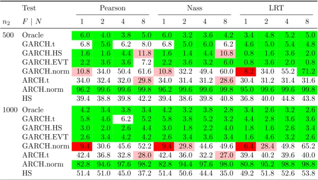
n2 = 500 andN = 8; this appears to show that the tests with more levels reveal deficiencies
Test Pearson Nass LRT n2 F |N 1 2 4 8 1 2 4 8 1 2 4 8 500 Oracle 6.0 4.0 3.8 5.0 6.0 3.2 3.6 4.2 3.4 4.8 5.2 5.0 GARCH.t 6.8 5.6 6.2 8.0 6.8 5.0 6.0 6.2 4.6 5.0 5.4 4.8 GARCH.HS 1.6 1.6 4.4 11.8 1.6 1.4 4.4 10.8 0.8 1.6 3.6 2.0 GARCH.EVT 2.2 3.6 3.6 7.2 2.2 3.6 3.2 6.0 0.8 3.6 2.0 0.8 GARCH.norm 10.8 34.0 50.4 61.6 10.8 32.2 49.4 60.0 8.2 34.0 55.2 71.2 ARCH.t 34.0 32.4 32.0 29.8 34.0 31.4 31.2 28.6 30.4 31.2 31.4 31.6 ARCH.norm 96.2 99.6 99.6 99.8 96.2 99.6 99.6 99.8 95.0 99.6 99.6 99.8 HS 39.4 38.8 39.8 42.2 39.4 38.6 39.8 40.8 36.8 40.0 44.8 43.8 1000 Oracle 4.2 3.4 3.8 3.4 4.2 3.2 3.8 2.8 3.4 2.6 3.2 2.6 GARCH.t 5.8 4.6 6.2 5.2 5.8 3.8 5.2 3.2 4.4 2.8 3.6 3.6 GARCH.HS 3.0 2.0 2.6 4.4 3.0 1.8 2.2 4.0 1.8 1.6 2.6 3.4 GARCH.EVT 2.6 3.4 4.2 4.2 2.6 3.4 3.6 3.4 1.6 4.6 3.2 2.6 GARCH.norm 9.4 30.6 45.6 52.2 9.4 29.8 44.6 49.6 6.4 28.4 49.8 65.2 ARCH.t 42.4 36.8 32.8 28.0 42.4 36.0 32.2 27.0 39.4 40.2 39.6 40.0 ARCH.norm 82.8 94.6 97.6 98.2 82.8 94.4 97.6 98.0 80.8 95.2 98.8 98.8 HS 51.4 51.0 45.0 37.2 51.4 50.6 44.4 35.0 49.2 51.8 52.6 53.8
Table 6: Estimated size and power of three different types of multinomial test (Pearson, Nass, likelihood-ratio test (LRT)) based on exceptions of N levels. Results are based on 500 replications of backtests of length 1000. The coloring scheme is the same as in Table 3.
4 A procedure to implicitly backtest ES
In view of the numerical results obtained in Section 3, we turn to the question of recom-mending a test procedure for use in practice. If we consider the simplicity of the test and the ease of explaining results to management and regulators to be the overriding factors, then a multinomial test with N = 4 or N = 8 can be recommended. This is an obvious improvement on a binomial test or a test using two quantiles, and is easy to implement with standard software. When consideringN = 4 orN = 8, we observe a similar general pattern for the three tests privided the backtest sample size exceeds 250. We would tend to rule out the LRT because of its relatively poor size and prefer the Nass test to the Pearson test, because of its more stable size and power. The choice of N = 4 or N = 8 for the Nass test will not impact the results very much because of this stability.
We can now propose an implicit backtest for ES, defining a decision criterion based on the multinomial approach we developed so far. Indeed, the ES estimate derived from a model that is not rejected by our multinomial test, is implicitly accepted by our backtest. Hence we can use the same rejection criterion for ES as for the null hypothesis H0 in the multinomial test.
The Basel Committee on Banking Supervision (2016) has proposed a traffic-light system for determining whether capital multipliers should be applied based on the results of a simple exception binomial test based on a backtest length of n1 = 250 days. We explain how the
traffic light system can be extended to any one of our multinomial tests and illustrate the results in the case when N = 2 (simply because this case lends itself to graphical display). Let B be the number of exceptions at the 99% level in one trading year of 250 days and let GB denote the cdf of a Binomial B(250,0.01) random variable. In the Basel system, if
GB(B) <0.95, then the traffic light is green and the basic multiplier of 1.5 is applied to a bank’s capital; this is the case provided B ≤ 4. If 0.95 ≤ GB(B) < 0.9999, then the light is yellow and an increased multiplier in the range [1.70,1.92] is applied; this is the case for
B ∈ {5, . . . ,9}. IfGB(B)≥0.9999, the light is red and the maximum multiplier 2 is applied; this occurs if B ≥10. A red light also prompts regulatory intervention.
We can apply exactly the same philosophy. In all our multinomial tests, the test statisticSN has a chi-squared distribution with some degree of freedom (sayθ) under the null hypothesis. LetGθdenote the cdf of a chi-squared distribution. IfGθ(SN)<0.95, we would set the traffic light to be green; if Gθ(SN)≥0.95, we would set the traffic light to be (at least) orange; if
Gθ(SN)≥0.9999, we would set the traffic light to be red. We could easily develop a system of capital multipliers for the orange zone based on a richer set of thresholds.
test that has been used is the Nass test. Obviously values ofN >2 correspond to cubes and hypercubes that are less easy to display, but we would use the same logic to assign a color based on the data (O0, O1, . . . , ON).
Figure 2: Traffic lights based on a trinomial test (N = 2) withn= 250,α1 = 0.975andα2= 0.9875.
O1 and O2 are the numbers of observations falling in the two upper bins (the lower bin contains
O0 = 250−O1−O2 observations). Cells are colored green unless the test p-value is less than or
equal 0.05, in which case they are either yellow (p-value greater than 0.0001) or red (p-value less than or equal 0.0001). O1 O2 0 1 2 3 4 5 6 7 8 9 10 11 12 13 0 1 2 3 4 5 6 7 8 9 10 11 12 13
5 Applying the backtest to real data
To illustrate the use of our multinomial test, we apply it to real data. We include three examples using different assets classes, different number of time periods and different block sizes, to understand better the situations in which our test gives significant results.
We consider first a hypothetical investment in the Standard & Poor’s 500 index where losses are given by the time series of daily log-returns. We conduct a backtest over the 40-year period from 1976–2016 carrying out a multinomial test in each 4-year period (approximately 1000 days) and comparing its power to that of a one-sided binomial LRT of VaR exceptions of the 99% level, which is the test that underlies the Basel traffic-light system. The results can be found in Table 7.
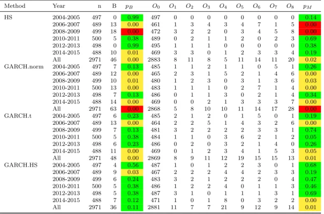
In the second example we consider an internationally diversified portfolio with investments in the S&P index, the FTSE index and the SMI index. This portfolio (also proposed as an example in McNeil et al. (2015), chapter 9), is subject to both equity and FX risk. Results are given in Table 8.
In a third example, we look at a long position in an in-the-money call option on the S&P 500 index. The option has a strike of 100 and a maturity of 1 year. We consider the situation where the stock is trading at 120, the interest rate is 1%, the annualized volatility is 30% and profits and losses are generated using log-returns of the S&P 500 index and the VIX volatility index; thus this example considers both equity and volatility risk. Results are given in Table 9. In this example and the previous example we use two-year blocks to increase the number of time periods, starting from 2004 (instead of 1976); this is dictated by the availability of the relevant time series data.
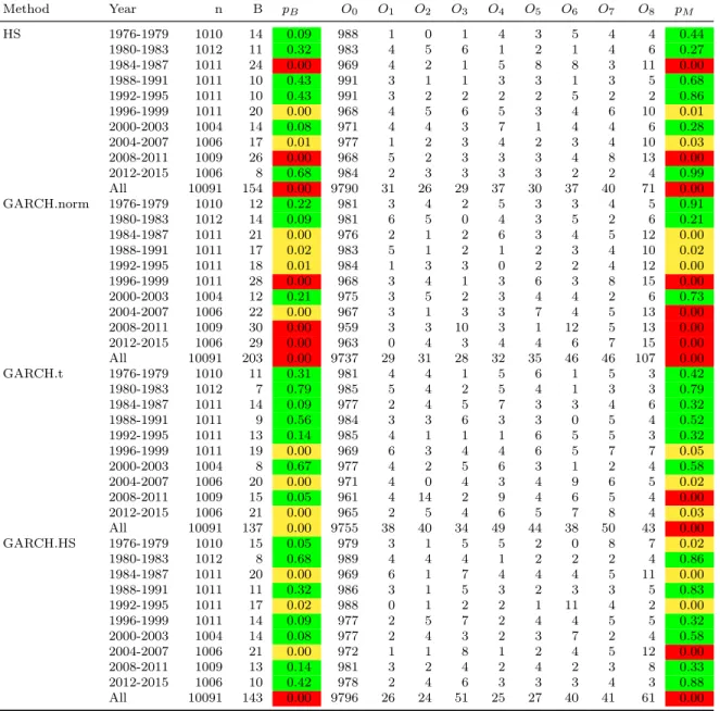
For the multinomial test, we choose the Nass test withN = 8 equally-spaced levels, starting as usual from α = 0.975. We give the results for four of the forecasters considered in Section 3.3: HS, GARCH.norm, GARCH.t, GARCH.HS. Note that for the GARCH.norm, GARCH.t and GARCH.HS methods we use a simple univariate dynamic risk estimation approach in which volatility is modelled at the level of the portfolio returns rather than the level of the underlying risk factors. In all methods a rolling window of n2 = 500 days is
used to derive one-step-ahead quantile estimates and these are compared with realized losses the next day. The parameters of the GARCH.norm and GARCH.t models are updated every 10 days. This is the same procedure as was used in the dynamic backtesting study of Section 3.3. Clearly, in order to initiate the analysis we need 500 days of data pre sample. In the three tables, the column markedB gives the number of exceedances of the 99% VaR estimate and the columns marked O0, . . . , ON give the observed numbers in equally-sized sells above the 97.5% level; pB andpM give thep-values for a one-sided binomial LRT at the 99% level and for a multinomial Nass test respectively.
We color the results according to the traffic-lights system described in Section 4 both within a single 4-year (or 2-year period), and over the whole period. Thus a p-value less than 0.05 leads to a yellow color and a p-value less than 0.0001 leads to a red color; both correspond to rejection of the null hypothesis.
It should be emphasized that, in contrast to all the other tables in this paper, Tables 7–9 contain p-values and not estimates of power or size. In interpreting the results we need to take into account the fact that each example is based on a single realization or sample path. Nevertheless, having demonstrated the superiority of the multinomial backtests withN ≥4 to the binomial test in a simulation study with 10,000 sample paths, we have much more faith in the p-values produced by the multinomial test than those provided by the binomial test, even when both have the same color. The color scheme is relatively crude with green covering the large range between 0.05 and 1 and the actualp-values can show differences between the two tests in evaluating the weight of evidence for good and bad modelling procedures that are not evident when we only consider the colors.
The general tendency across the three analyses is for slightly more yellow and red lights to be illuminated when the multinomial test is used. Over many further experiments this
tendency would be reinforced.
We observe that for the HS and GARCH.norm forecasters (which would be considered in general to be poor methods), the binomial and multinomial tests lead to broadly similar conclusions with slightly more pronounced rejection of these methods for pm than pB (see e.g. GARCH.norm in the period 2004-07, in Table 7).
The results of the HS forecaster are rejected in 4 out of 10 periods in Table 7, 3 out of 6 period in Table 8 and 2 out of 6 in Table 9), as well as over the whole period in all cases. The results of the GARCH.norm forecaster are rejected in 7 out of 10 periods in Table 7, 4 out of 6 in Table 8 and 1 out of 6 in Table 9), as well as for the whole period in all cases. The traffic-light coloring is mostly the same for both tests, but with more red lights for the multinomial test.
It is for the other two forecasters that the increased power of the multinomial test is apparent in particular when the block size is sufficiently large. When considering the GARCH.t forecaster, we observe that, in the case of Table 7, the multinomial test rejects in the period 2008–2011, which contains the 2008 financial crisis, whereas the binomial test does not. The GARCH.t model may be neglecting the asymmetry of the return process in this volatile period, a phenomenon which is detected by the multinomial test which also rejects the results of this forecaster over the whole period. When looking at shorter block sizes in the two other examples, we no longer observe this effect, showing the impact of the choice of block size. This is in line with what we found in the simulation study regarding the role of the sample size: to achieve satisfactory power requires enough data.
In the case of the GARCH.HS forecaster and the S&P500, the multinomial test also rejects in one additional period (1976–1979) and with higher significance in the period 2004–2007 (red versus yellow). For the period 2008–2011, the GARCH.HS forecaster seems to perform
better than the parametric forecasters. In the other two examples there are periods where the two tests lead to slightly different results for the GARCH.HS forecaster; these are 2006–07 and 2014–15 in Table 8 and 2004–05, 2006–07 and 2014–15 in Table 9.
To conclude, while these examples are based on single time series, they give an indication of the increased power of the multinomial test over the binomial. The tabulated numbers between each quantile estimate O1, . . . , ON give additional information about the region of the tail in which the models fail; in a backtest of lengthn = 1000 withN = 8 levels starting atα = 0.975, the expected numbers are 25/3≈3 in each cell.
Method Year n B pB O0 O1 O2 O3 O4 O5 O6 O7 O8 pM HS 1976-1979 1010 14 0.09 988 1 0 1 4 3 5 4 4 0.44 1980-1983 1012 11 0.32 983 4 5 6 1 2 1 4 6 0.27 1984-1987 1011 24 0.00 969 4 2 1 5 8 8 3 11 0.00 1988-1991 1011 10 0.43 991 3 1 1 3 3 1 3 5 0.68 1992-1995 1011 10 0.43 991 3 2 2 2 2 5 2 2 0.86 1996-1999 1011 20 0.00 968 4 5 6 5 3 4 6 10 0.01 2000-2003 1004 14 0.08 971 4 4 3 7 1 4 4 6 0.28 2004-2007 1006 17 0.01 977 1 2 3 4 2 3 4 10 0.03 2008-2011 1009 26 0.00 968 5 2 3 3 3 4 8 13 0.00 2012-2015 1006 8 0.68 984 2 3 3 3 3 2 2 4 0.99 All 10091 154 0.00 9790 31 26 29 37 30 37 40 71 0.00 GARCH.norm 1976-1979 1010 12 0.22 981 3 4 2 5 3 3 4 5 0.91 1980-1983 1012 14 0.09 981 6 5 0 4 3 5 2 6 0.21 1984-1987 1011 21 0.00 976 2 1 2 6 3 4 5 12 0.00 1988-1991 1011 17 0.02 983 5 1 2 1 2 3 4 10 0.02 1992-1995 1011 18 0.01 984 1 3 3 0 2 2 4 12 0.00 1996-1999 1011 28 0.00 968 3 4 1 3 6 3 8 15 0.00 2000-2003 1004 12 0.21 975 3 5 2 3 4 4 2 6 0.73 2004-2007 1006 22 0.00 967 3 1 3 3 7 4 5 13 0.00 2008-2011 1009 30 0.00 959 3 3 10 3 1 12 5 13 0.00 2012-2015 1006 29 0.00 963 0 4 3 4 4 6 7 15 0.00 All 10091 203 0.00 9737 29 31 28 32 35 46 46 107 0.00 GARCH.t 1976-1979 1010 11 0.31 981 4 4 1 5 6 1 5 3 0.42 1980-1983 1012 7 0.79 985 5 4 2 5 4 1 3 3 0.79 1984-1987 1011 14 0.09 977 2 4 5 7 3 3 4 6 0.32 1988-1991 1011 9 0.56 984 3 3 6 3 3 0 5 4 0.52 1992-1995 1011 13 0.14 985 4 1 1 1 6 5 5 3 0.32 1996-1999 1011 19 0.00 969 6 3 4 4 6 5 7 7 0.05 2000-2003 1004 8 0.67 977 4 2 5 6 3 1 2 4 0.58 2004-2007 1006 20 0.00 971 4 0 4 3 4 9 6 5 0.02 2008-2011 1009 15 0.05 961 4 14 2 9 4 6 5 4 0.00 2012-2015 1006 21 0.00 965 2 5 4 6 5 7 8 4 0.03 All 10091 137 0.00 9755 38 40 34 49 44 38 50 43 0.00 GARCH.HS 1976-1979 1010 15 0.05 979 3 1 5 5 2 0 8 7 0.02 1980-1983 1012 8 0.68 989 4 4 4 1 2 2 2 4 0.86 1984-1987 1011 20 0.00 969 6 1 7 4 4 4 5 11 0.00 1988-1991 1011 11 0.32 986 3 1 5 3 2 3 3 5 0.83 1992-1995 1011 17 0.02 988 0 1 2 2 1 11 4 2 0.00 1996-1999 1011 14 0.09 977 2 5 7 2 4 4 5 5 0.32 2000-2003 1004 14 0.08 977 2 4 3 2 3 7 2 4 0.58 2004-2007 1006 21 0.00 972 1 1 8 1 2 4 5 12 0.00 2008-2011 1009 13 0.14 981 3 2 4 2 4 2 3 8 0.33 2012-2015 1006 10 0.42 978 2 4 6 3 3 3 4 3 0.88 All 10091 143 0.00 9796 26 24 51 25 27 40 41 61 0.00
Table 7: Results of multinomial and binomial backtests applied to an investment in the S&P index. B gives the number of exceedances of the 99% VaR estimate and the columns O0, . . . , ON give the observed numbers in cells defined by settingα= 0.975. pB andpM give thep-values for a one-sided binomial LRT and a multinomial Nass test respectively. p-values less than 0.05 are colored green; p-values in (0.0001,0.05] are yellow;p-values less than or equal 0.0001 are red.
Method Year n B pB O0 O1 O2 O3 O4 O5 O6 O7 O8 pM HS 2004-2005 497 0 0.99 497 0 0 0 0 0 0 0 0 0.14 2006-2007 489 13 0.00 461 1 3 4 3 4 7 1 5 0.00 2008-2009 499 18 0.00 472 3 2 2 0 3 4 5 8 0.00 2010-2011 500 5 0.38 489 0 2 1 1 2 0 2 3 0.69 2012-2013 498 0 0.99 495 1 1 1 0 0 0 0 0 0.38 2014-2015 488 10 0.01 469 3 3 0 1 2 3 3 4 0.19 All 2971 46 0.00 2883 8 11 8 5 11 14 11 20 0.02 GARCH.norm 2004-2005 497 7 0.13 485 1 1 2 1 1 0 5 1 0.26 2006-2007 489 12 0.00 465 2 3 1 5 2 1 4 6 0.00 2008-2009 499 10 0.01 480 1 2 3 0 3 1 3 6 0.03 2010-2011 500 13 0.00 483 1 1 1 0 2 7 1 4 0.00 2012-2013 498 7 0.13 486 0 1 1 3 0 2 1 4 0.34 2014-2015 488 14 0.00 469 0 0 2 1 3 3 3 7 0.00 All 2971 63 0.00 2868 5 8 10 10 11 14 17 28 0.00 GARCH.t 2004-2005 497 6 0.23 485 2 1 2 0 1 5 0 1 0.19 2006-2007 489 13 0.00 464 2 2 5 1 4 3 2 6 0.00 2008-2009 499 7 0.13 481 3 2 2 2 2 3 3 1 0.74 2010-2011 500 5 0.38 484 1 1 0 3 6 2 1 2 0.05 2012-2013 498 6 0.23 486 0 2 0 3 2 1 4 0 0.26 2014-2015 488 11 0.00 469 0 1 2 3 4 1 5 3 0.05 All 2971 48 0.00 2869 8 9 11 12 19 15 15 13 0.01 GARCH.HS 2004-2005 497 4 0.56 487 1 0 1 2 2 3 0 1 0.68 2006-2007 489 9 0.03 467 2 2 2 4 4 2 3 3 0.19 2008-2009 499 6 0.24 483 3 2 1 2 2 2 0 4 0.47 2010-2011 500 5 0.38 486 1 2 2 4 0 1 1 3 0.46 2012-2013 498 5 0.38 487 3 1 0 1 1 1 3 1 0.69 2014-2015 488 7 0.12 471 1 0 1 8 0 3 2 2 0.00 All 2971 36 0.11 2881 11 7 7 21 9 12 9 14 0.01
Table 8: Results of multinomial and binomial backtests applied to a portfolio subject to equity and FX risk. B gives the number of exceedances of the 99% VaR estimate and the columnsO0, . . . , ON give the observed numbers in cells defined by setting α = 0.975. pB and pM give the p-values for a one-sided binomial LRT and a multinomial Nass test respectively. p-values less than 0.05 are colored green;p-values in (0.0001,0.05] are yellow; p-values less than or equal 0.0001 are red.