Statistical Methods for Multivariate Meta-Analysis of
Diagnostic Tests
A DISSERTATION
SUBMITTED TO THE FACULTY OF THE GRADUATE SCHOOL OF THE UNIVERSITY OF MINNESOTA
BY
Xiaoye Ma
IN PARTIAL FULFILLMENT OF THE REQUIREMENTS FOR THE DEGREE OF
Doctor of Philosophy
Advised by Prof. Haitao Chu
c
Xiaoye Ma 2015 ALL RIGHTS RESERVED
Acknowledgements
I would like to express the deepest appreciation to my advisor, Dr. Haitao Chu, for his excellent guidance and persistent support throughout my master and doctoral study, for his patience, enthusiasm, and immense knowledge. I am extremely grateful that Dr. Haitao Chu agreed to be my advisor since my Master’s study, when I was enlightened at the first glance of research. My journey of Ph.D. study is challenging, but with his persistent support and sincere advice, it turned out to be extremely rewarding and memorable. I am truly thankful to have Dr.Bradley P. Carlin be my committee chair. His intelligence and expertise has invaluable input in my dissertaion. I am also grateful that Dr.Bradley P. Carlin referred me to Dr.David Ohlssen at Novartis for a summer internship position. Without this experience I would not be able to find a full-time job as smoothly. Many thanks also go to my committee members Dr.Wei Pan and Dr.Richard MacLehose, for their friendly guidance, thought-provoking suggestions, and invaluable input. Thanks go to Dr.Muhammad Fareed K. Suri, who got me involved in his interesting research project. Thanks to all professors who taught me classes in my graduate study and all my classmates and officemates who shared ideas, discussions and help with each other’s difficulties.
I also want to send my thanks to my family overseas. Thank you mom and dad for sending me abroad to study, trusting me to pursue my dream, which opened a gate to an incredibly amazing life. Thank you grandpas and grandmas, in China and in heaven, for your endless care, and your lovely effort to try to remember name of my school. At last, special thanks to my husband, Chuan Shi. Thank you for always staying by my side, facing all difficulties together and helping me bulid my confidence. I can always feel your love and support no matter how far apart we are.
Dedication
To my husband, Chuan Shi, and my parents Lin Ma and Xun Sun, for their infinite love, trust and support.
Abstract
Accurate diagnosis is often the first step towards the treatment and prevention of disease. Many quantitative comparisons of diagnostic tests have relied on meta-analyses, which are statistical methods to synthesize all available information in various clinical studies. In addition, in order to effectively compare the growing number of diagnostic tests for a specific disease, innovative and efficient statistical methods to simultaneously compare multiple diagnostic tests are urgently needed for physicians and patients to make better decisions.
In the literature of meta-analysis of diagnostic tests (MA-DT), discussions have been focused on statistical models under two scenarios: (1) when the reference test can be considered a gold standard, and (2) when the reference test cannot be considered a gold standard. We present an overview of statistical methods for MA-DT in both scenarios. This dissertation covers both conventional and advanced multivariate approaches for the first scenario, and a latent class random effects model when the reference test itself is imperfect.
As study design and populations vary, the definition of disease status or severity could differ across studies. A trivariate generalized linear mixed model (TGLMM) has been proposed to account for this situation; however, its application is limited to cohort studies. In practice, meta-analytic data is often a mixture of cohort and case-control studies. In addition, some diagnostic accuracy studies only select a subset of samples to be verified by the reference test, which is known as potential source of partial verification bias in single studies. The impact of this bias on a meta-analysis has not been investigated. We propose a novel hybrid Bayesian hierarchical model to combine cohort and case-control studies, and correct partial verification bias at the same time.
A recent paper proposed an intent-to-diagnose approach to handle non-evaluable in-dex test results, and discussed several alternative approaches. However, no simulation studies have been conducted to test the performance of the methods. We propose an extended TGLMM to handle non-evaluable index test results, and examine the perfor-mance of the intent-to-diagnose approach, the alternative approaches, and the proposed approach by extensive simulation studies.
monly used: 1) the multiple test comparison design; 2) the randomized design; and 3) the non-comparative design. Existing MA-DT methods have been focused on evaluating the performance of a single test by comparing it with a reference test. The increasing number of available diagnostic instruments for a disease condition and the different study designs being used have generated the need to develop an efficient and flexible meta-analysis framework to combine all designs for simultaneous inference. We develop a missing data framework and a Bayesian hierarchical model for network meta-analysis of diagnostic tests (NMA-DT), and offer key advantages over traditional MA-DT meth-ods.
Contents
Acknowledgements i
Dedication ii
Abstract iii
List of Tables viii
List of Figures x
1 Introduction 1
1.1 Current development and challenges in meta-analysis of diagnostic tests
(MA-DT) . . . 2
1.1.1 Literature review in MA-DT . . . 2
1.1.2 Mixture of case-control and cohort studies . . . 3
1.1.3 Partial verification bias . . . 4
1.1.4 Non-evaluable subjects . . . 6
1.2 Network meta-analysis of diagnostic tests (NMA-DT) . . . 7
2 Statistical methods for multivariate MA-DT 10 2.1 Statistical methods when the reference test is a gold standard . . . 10
2.1.1 The summary ROC method . . . 11
2.1.2 A bivariate approach based on LMM . . . 13
2.1.3 The hierarchical summary ROC approach . . . 14
2.1.4 The bivariate generalized linear mixed model (GLMM) . . . 16
2.2 Statistical methods when the reference test is not a gold standard . . . 18
2.3 Discussion . . . 22
3 A hybrid Bayesian hierarchical model combining cohort and case-control studies for meta-analysis of diagnostic tests: Accounting for partial verification bias 24 3.1 Bayesian hierarchical model . . . 25
3.1.1 Notations . . . 25
3.1.2 The likelihood with random effects accounting for heterogeneity . 28 3.1.3 Bayesian posterior sampling approach . . . 29
3.2 Simulation . . . 30
3.2.1 Simulation design . . . 30
3.2.2 Simulation results . . . 31
3.3 Case study . . . 35
3.3.1 Meta-analysis of gadolinium-enhanced MRI in detecting lymph node metastases . . . 35
3.3.2 Meta-analysis of adrenal fluorine-18 fluorodeoxyglucose (FDG) positron emission tomography (PET) in characterizing adrenal masses . . . 43
3.4 Discussion . . . 44
4 A trivariate meta-analysis of diagnostic studies accounting for preva-lence and non-evaluable subjects: re-evaluation of the meta-analysis of coronary CT angiography studies 47 4.1 Methods . . . 48
4.2 Simulations . . . 51
4.2.1 Simulation Scenarios . . . 51
4.2.2 Simulation Results . . . 52
4.3 Re-evaluation of the meta-analysis of coronary CT angiography studies . 55 4.4 Conclusions . . . 55
5 A Bayesian Hierarchical Model for Network Meta-analysis of
Diagnos-tic Tests 59
5.1 Motivating studies . . . 60
5.1.1 NMA of deep vein thrombosis (DVT) tests . . . 60
5.1.2 NMA of latent tuberculosis (TB) tests . . . 61
5.2 A unified statistical framework . . . 61
5.2.1 Likelihood function . . . 62
5.2.2 Random effects and prior specifications . . . 63
5.2.3 Model implementation and a Bayesian ranking procedure . . . . 64
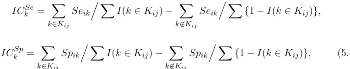
5.2.4 A measure of inconsistency . . . 65
5.3 Case study results and sensitivity analyses . . . 66
5.3.1 NMA of DVT tests . . . 66
5.3.2 NMA of latent TB tests . . . 72
5.4 Simulation Studies . . . 76
5.4.1 Simulation setups . . . 76
5.4.2 Simulation results . . . 78
5.5 Discussion . . . 78
6 Conclusions 82 6.1 Summary of major findings . . . 82
6.2 Limitations and extensions to future work . . . 83
References 85
Appendix A. Data for MA of gadolimium-enhanced MRI and MA of
FDG PET 97
Appendix B. Additional simulation results for hybrid GLMM 100
Appendix C. Glossary for abbreviations 103
List of Tables
1.1 2×2 table for a toy example . . . 2
2.1 2 by 2 table forith study . . . 11
2.2 2 by 2 table forith study accounting for prevalence . . . 18
2.3 2 by 2 table when the reference test is not a gold standard . . . 20
3.1 Data display for theith study when it is a cohort study and when it is a case-control study. . . 27
3.2 Summary of 2000 simulations with data generated from settings with 30 studies, true Se (Sp)=0.7 (0.8) and different correlation assumptions. . 33
3.3 Median estimates and 95% CI for meta-analysis of MRI: comparing two prior families (the scaled and unscaled inverse Wishart prior) and com-paring different choices of the Wishart prior parameterR. . . 37
3.4 Median estimates and 95% CI for meta-analysis of FDG PET: comparing the hybrid GLMM and model 3.2 where partial verification is ignored . 44 4.1 3×2 table accounting for prevalence and missing index test results. . . 49
4.2 Simulation results under three scenarios of MAR assumption: equal or unequal missing probabilities for the diseased and non-diseased groups. . . 54
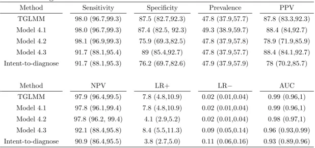
4.3 Median estimates and 95% confidence intervals (in brackets) for param-eter estimates using different methods . . . 57
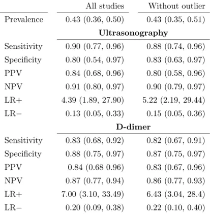
5.1 Meta-analysis of DVT tests: median estimates and 95% CIs. Estimates from models using all studies under “All studies” are compared to esti-mates excluding an “outlier” study 5 under “Without outlier”. . . 67
5.2 Meta-analysis of DVT tests: median parameter estimates and 95% CIs under different missingness assumptions. . . 71
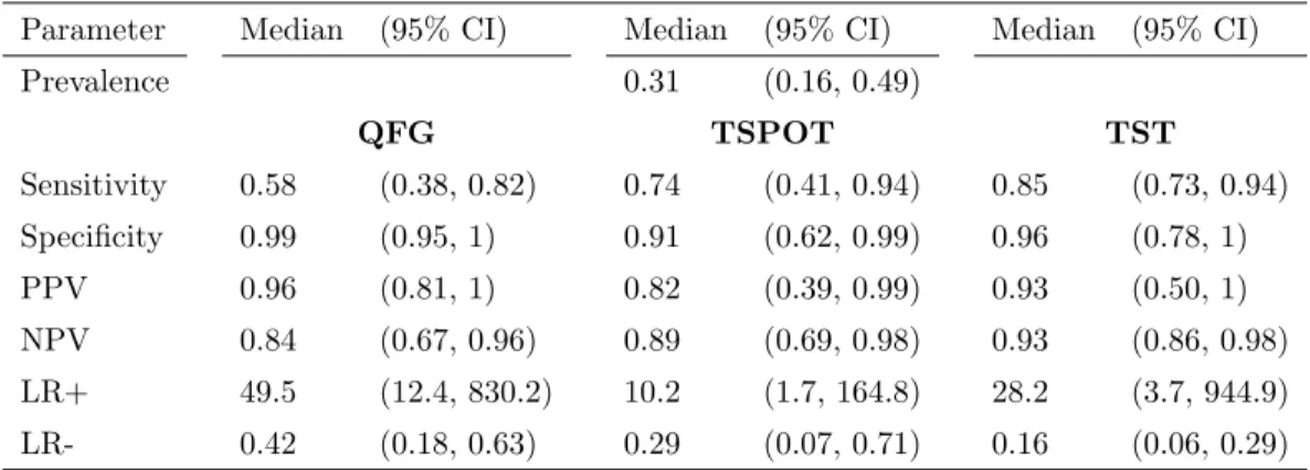
5.3 Meta-analysis of latent TB tests: posterior medians and 95% CI’s . . . . 73
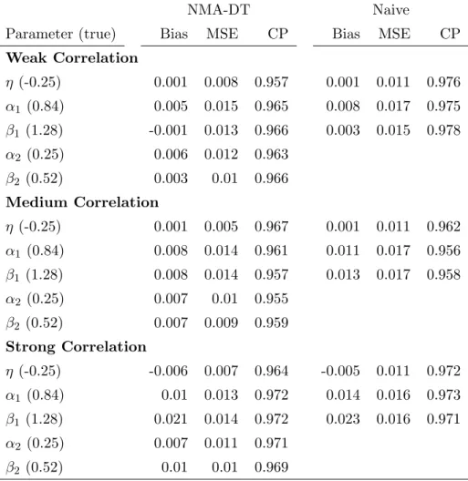
5.4 Meta-analysis of latent TB tests: posterior estimates under different miss-ingness assumptions. . . 76 5.5 Simulation results: bias, mean square error (MSE) and 95% CI coverage
probabilities (CP) of the estimates for fixed effects η, α1, β1, α2, β2. Es-timates from the proposed NMA-DT model and the “naive” method are compared forT1. . . 79 A.1 Data for the meta-analysis of gadolinium-enhanced MRI in detecting
lymph node metastases . . . 98 A.2 Data for the meta-analysis of FDG PET in characterizing adrenal masses 99 B.1 Summary of 2000 simulations with data generated from settings with 30
studies and true Se (Sp)=0.9 (0.95). . . 101 B.2 Summary of 2000 simulations with data generated from settings with 10
studies and true Se (Sp)=0.7 (0.8). . . 101 B.3 Summary of 2000 simulations with data generated from settings with 10
studies and true Se (Sp)=0.9 (0.95). . . 102
List of Figures
3.1 Quantile contours of posterior densities from estimates of the meta-analysis of gadolinium-enhanced MRI in detecting lymph node metastases assum-ing scaled Wishart prior. A-D plot posterior Se versus prevalence (π), Sp versusπ, Se versus Sp and PPV versus NPV, respectively, at quantile levels 0.25, 0.5, 0.75, 0.9 and 0.95. . . 39 3.2 SROC curves from the Hybrid GLMM and the bivariate GLMM using
MLE approach. Solid lines are the SROC curve from the hybrid GLMM estimates and the 95% prediction region for the summary point estimates of Se and Sp. Dashed lines are the SROC curve from the bivaraite es-timates and the 95% prediction region for the summary point eses-timates of Se and Sp. Black and gray circles are the observed Se and Sp from studies with and without missing counts, respectively. Red and blue tri-angles are the posterior estimates of Se and Sp from the Hybrid GLMM and the Bivariate GLMM ignoring partial verification, respectively. . . . 40 3.3 Density plots of posterior estimates of the meta-analysis of
gadolinium-enhanced MRI in detecting lymph node metastases under different prior assumptions. Panel A plots posterior densities of Se, Sp and prevalence (π). Panel B plots posteriors densities of PPV and NPV. . . 42
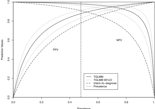
4.1 Overall PPV and NPV plot based on the extended TGLMM (denoted by “TGLMM”) and the intent-to-diagnose approach. The solid and dashed lines are the overall estimates of PPV and NPV from the extended TGLMM and the intent-to-diagnose approach corresponding to different prevalences ranging from 0 to 1, respectively. The dotted lines are the 95% confidence intervals of PPV and NPV estimates from the extended TGLMM approach. The vertical dashed line is the overall prevalence estimates from the meta-analysis of coronary CT angiography studies. . 56 5.1 Meta-analysis of DVT tests: posterior densities and study-specific posterior
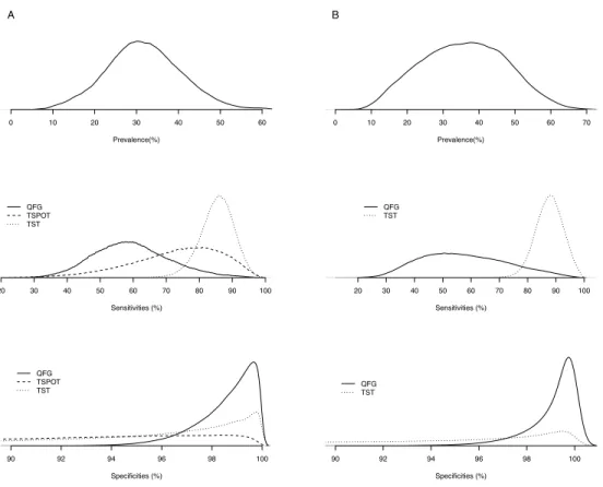
es-timates. The left column plots posterior densities and the right column plots study-specific posterior medians and their 95% CIs for prevalence, sensitivities and specificities of ultrasonography and D-dimer tests. Circles represent study-specific posterior medians and solid and dashed lines denote the corresponding 95% CIs when the test is included in the study and not included (imputed by MCMC sampling), respectively. A red line indicates a potential outlier study. Dotted lines indicate overall posterior medians across studies. . . 68 5.2 Meta-analysis of latent TB tests: panel A plots the posterior densities of
parameters using all studies; Panel B plots the posterior densities when studies reporting the TSPOT test are excluded. . . 74
Chapter 1
Introduction
Accurate diagnosis of a disease is often the first step toward its treatment and preven-tion. The performance of a binary test of interest (candidate or index test) is commonly compared to a reference test (preferably a “gold standard” test), then measured by a pair of indices such as sensitivity (Se) and specificity (Sp). Sensitivity is defined as the probability of testing positive given a person is diseased, and specificity is defined as the probability of testing negative given a person is disease-free[1]. For a toy example, ultrasound is the candidate or index test in diagnosing rotator cuff tears, and the gold standard test is arthroscopic surgery. In one study, to estimate the Se and Sp of ultra-sound, a group of participants are tested by both ultrasound and the gold standard, and test outcomes are compared in a cross-tabulated 2 ×2 table (Table 1.1). In this study, Se is estimated as P r(Ultrasound = +|Diseased) = 80/100 = 0.8 and Sp is estimated as P r(Ultrasound = −|Non-diseased) = 180/200 = 0.9. Other frequently used indices include positive and negative predictive values (PPV and NPV), and positive and neg-ative diagnostic likelihood ratios (LR+ and LR−). PPV is defined as the probability of being diseased given a positive index test result, and NPV is defined as the proba-bility of being disease-free given a negative index test result. In this example, PPV is estimated as P r(Diseased|Ultrasound = +) = 80/100 = 0.8 and NPV is estimated as P r(Non-diseased|Ultrasound =−) = 180/200 = 0.9.
The growing number of assessment instruments, as well as a rapid escalation in trial costs, has generated an increasing need for scientifically rigorous comparisons of the di-agnostic tests in clinical practice. Meta-analysis of diagnostic test (MA-DT)is a useful
2
Table 1.1: 2× 2 table for a toy example Arthroscopic
Ultrasound + (Diseased) −(Non-diseased) Total
+ 80 20 100
− 20 180 200
Total 100 200 300
tool to combine evidence on diagnostic accuracies from multiple studies. Compared to conventional meta-analyses of controlled clinical trials, it has several additional statis-tical challenges that have been extensively studied in the literature, such as correlation between test accuracy indices and heterogeneity of test performance across studies. Other important topics in MA-DT, such as partial verification and mixture of study designs remain challenging.
The increasing number of available diagnostic instruments for a disease condition has generated a need to develop an efficient and flexible meta-analysis framework for simultaneous inference. As a result, in order to effectively compare multiple diagnostic tests, extending MA-DT from studying the performance of a single test, to enabling simultaneous comparison of multiple test performance by a framework ofnetwork meta-analysis of diagnostic tests (NMA-DT), is urgently needed for physicians and patients to make better decisions in selecting tests.
1.1
Current development and challenges in meta-analysis
of diagnostic tests (MA-DT)
1.1.1 Literature review in MA-DT
In MA-DT, there is a great potential for heterogeneity due to differences in such things as disease prevalence, study population characteristics, laboratory methods, and study designs. While some study level covariates such as the mean age may explain some of the variability, random effects models are commonly recommended to account for other unobserved sources of variation. When a reference test can be considered as a gold standard, several meta-analysis methods are available to account for this
heterogeneity[2, 3, 4, 5, 6, 7, 8, 9, 10, 11]. Specifically, random effects models, including the hierarchical summary receiver operating characteristic model [2] and bivariate ran-dom effects meta-analysis on sensitivities and specificities[4, 10, 11], which are identical in some situations, have been recommended [5, 8, 12]. Indeed, extensive examples and simulations demonstrated that bivariate random-effects meta-analysis offers numerous advantages over separate univariate meta-analysis [13, 14]. In general, generalized linear mixed models (GLMM), which use the exact binomial likelihood, often perform better than the linear mixed models which use a normal approximation[10, 15]. In addition, a trivariate GLMM (TGLMM) was also proposed to jointly model the disease prevalence, sensitivities and specificities[16].
In practice, disease status is often measured by a reference test that is subject to nontrivial measurement error. This leads to a setting “without a gold standard”. When the reference test is subject to measurement error, the evaluation of diagnostic tests in a meta-analysis setting becomes more challenging. Only a few articles have described meta-analysis models for diagnostic tests in the absence of a gold standard. Walter et al.[17] discussed a latent class model for a meta-analysis of two diagnostic tests assuming varying prevalence, but constant sensitivity and specificity across studies. A more general latent class random effects model by Chu et al.[18] assumes sensitivity and specificity of both tests as well as prevalence to be random effects. Sadatsafavi et al.[19] presented a model where conditional dependence between tests is allowed but other than prevalence, only one of the sensitivity or specificity can be implemented as random effects. Dendukuri et al.[20] presented a Bayesian meta-analysis for the accuracy of a test for tuberculous pleuritis in the absence of a gold standard. In this thesis, we will perform a systematic review and comparison of the above mentioned methods.
1.1.2 Mixture of case-control and cohort studies
As introduced in the last section, the paired indices measuring diagnostic test perfor-mance are potentially correlated and heterogeneous across studies, such that bivariate random effects models on sensitivities and specificities have been recommended to ac-count for such correlation and heterogeneity [5, 10, 4]. In addition, because the clas-sification of disease status is typically based on a continuum of measurable traits, and such continuous traits not only determine disease prevalence, but also misclassification
4 rates (subjects with true levels close to the cut-point are more likely to be misclassified), sensitivities and specificities can be correlated with study prevalences [21]. TGLMMs on prevalence, sensitivities and specificities were proposed to account for such correlations [22]. However, many meta-analyses of diagnostic tests in practice contain both cohort and case-control study designs [23]. Using cohort design, a study first tests participants with the index test, and then confirms disease status with the gold standard[24]. In case-control design studies, groups of patients with and without disease are identified before performing the index test [25]. Thus, case-control studies cannot be used to estimate disease prevalence, and direct application of the trivariate random effects models has been restricted to a meta-analysis with cohort studies only. In such situations, ignoring the information on prevalence to fit the bivariate random effects model [10, 4, 8, 11] on Se and Sp, or excluding case-control studies to fit the trivariate random effects model [22] on prevalence, can potentially lead to a substantial loss of information contained in the data. For example, the former approach ignores disease prevalence information and the correlations between disease prevalence Se and Sp, which can lead to incorrect estimation of PPV and NPV.
1.1.3 Partial verification bias
Partial verification is a common and important potential source of bias that usually arises when the selection of samples to be tested by a reference standard test is affected by the results of a diagnostic test [26, 27]. As stated in the quality assessment tool for diagnostic accuracy studies (QUADAS), partial verification bias occurs when not all of the study group receive confirmation of the diagnosis by the reference standard [28]. As an illustration, let us use the previous example in Table 1.1 and assume that true Se and Sp of ultrasound are 0.8 and 0.9, respectively and no sampling variation. However, 80% of the subjects with ultrasound positive outcomes are verified, while only 20% of the subjects with ultrasound negative outcomes are verified by the gold standard. Let ntd denote the number of subjects with test results T = t and disease status Dis =d (t, d= 0,1, m indicating negative, positive and missing results, respectively). We will have n11 = 64, n01 = 4, n00 = 36, n10 = 16, n1m = 20 and n0m = 160. Now, if we only use verified samples, we overestimate Se as Sec = n11/(n11 +n01) = 0.94
magnitude of such bias depends on selection probabilities [29]. To avoid such bias, ideally, all subjects should be verified. However, due to some practical issues such as ethical and economic considerations, partial verification is ubiquitous. In a systematic review of bias and variation in meta-analysis of diagnostic accuracy studies, 15 out of 31 (48%) meta-analyses contain at least one study with partial verification [29]. Thus, it is important to adjust for partial verification bias in meta-analysis of diagnostic tests [29, 30].
Methods to adjust for verification bias in a single study are widely published. Most of the methods are built upon the missing at random (MAR) assumption, when the decision to ascertain disease status only depends on the observed index test result, T. Violations of this condition can happen when, for example, subjects with family disease history are more likely to verify their desease status[1]. Begg and Greenes [31] proposed a simple method based on Bayes theorem. Other methods such as multiple imputation, direct maximum likelihood, or Bayesian approaches have been proposed [32, 33, 34, 35, 36, 27]. These methods give unbiased estimates of Se and Sp for individual studies, instead of recovering missing counts of subjects. Thus we would not be able to apply the exact binomial likelihood assumption for a GLMM approach under meta-analysis settings. Few sensitivity meta-analysis methods are available under the assumption of Missing Not At Random (MNAR), i.e., the probability of being verified by a reference standard depends on the unobserved data[37, 38].
On the other hand, only limited papers are available on methods to adjust verifica-tion bias in a meta-analysis setting. De Groot et al. [39] extended the Bayes theorem method to adjusting for this bias in meta-analysis of diagnostic tests with nominal outcomes. A two-stage Bayesian approach was described, where in the 1st stage the probability distribution of the index test was calculated and in the 2nd stage PPV and NPV are calculated using observed data based on their unbiasedness property under the MAR assumption [1]. Bayes theorem is then applied to achieve pooled sensitivity and specificity estimates. A few papers have discussed the missing data problem caused by imperfect reference standards, but these papers are not aimed at partial verification problems specifically. Previously introduced papers by Chu et al. [18] and Sdatsafavi et al. [19] disscuss models for such a scenario.
6
1.1.4 Non-evaluable subjects
Most papers in the literature have discussed missing reference test outcomes (missing disease status) and how to correct such bias, known as partial verification bias[31, 39, 34, 26]. However, index test outcomes can be non-evaluable as well, especially for tests yielding dichotomous results, and different situations were discussed where index test result can be non-evaluable: uninterpretable, intermediate and indeterminate [40, 41].
For a single study, there are many discussions about how to deal with non-evaluable index test outcomes, such as excluding them [42], grouping them with positive or neg-ative outcomes[42, 40], or using a 3×2 table to report them as an extension of the standard 2×2 table[42]. On the other hand, in meta-analysis, there is little discussion of how to deal with missing index test outcomes[41]. The “classic” 2×2 table models such as the bivariate linear mixed models[2, 11, 5, 43, 4, 8], bivariate GLMM[10, 44, 45] and TGLMM [22] ignore missing index test outcomes. Recently, a paper by Schuetz et al.[41] discussed this issue by studying different approaches dealing with index test non-evaluable subjects. The paper conducted a meta-analysis of coronary CT angiography studies and presented an intent-to-diagnose approach together with three commonly applied alternative approaches. The intent-to-diagnose approach takes non-evaluable diseased subjects as false positives and non-diseased subjects as false negatives such that sensitivity and specificity won’t be overestimated. The other three alternative ap-proaches in Schuetz et al.[41] are described in Chapter 4. The authors concluded that excluding the index test non-evaluable subjects leads to over-estimation of sensitivity and specificity and recommended the conservative intent-to-diagnose approach by treat-ing non-evaluable diseased subjects as false negatives and non-evaluable non-diseased subjects as false positives. However, no simulation studies have been conducted to evaluate the performance of these approaches.
We can treat index test non-evaluable subjects as missing data. Schuetz et al.[41] concluded that sensitivity and specificity could be over-estimated by excluding non-evaluable subjects. In fact, under a reasonable general assumption, MAR, exclud-ing non-evaluable subjects can provide unbiased estimates of them. A special case of MAR is missing completely at random (MCAR), where missingness is indepen-dent of both observed and unobserved variables [46]. Under MAR, T and M are
independent given disease status Dis, where M = 1,0 indicates missingness of in-dex test outcome. Hence, excluding non-evaluable subjects will have unbiased esti-mates of Se and Sp: Sec = P r(T = 1|Dis = 1, M = 0) = P r(T = 1|Dis = 1) and
c
Sp = P r(T = 0|Dis = 0, M = 0) = P r(T = 0|Dis = 0). Similarly, positive and neg-ative likelihood ratios (LR+ and LR−) and area under the curve (AUC) estimates are unbiased too. Under MCAR, P r(M = 1|Dis = 1) =P r(M = 1|Dis = 0), and hence disease prevalence (π) estimate is also unbiased if non-evaluable subjects are excluded. However, when missing probabilities are not equal between diseased and non-diseased participants, disease prevalence estimate can be biased if non-evaluable subjects are excluded, leading overall estimates of PPV and NPV to be biased. PPV and NPV are generally preferred by clinicians as measurements of how well a test predicts true disease status because their interpretations are more intuitive: PPV is the probability that a subject with positive intex test result is truly diseased and NPV is the probability that a subject with negative intex test result is truly non-diseased[1]. However, none of the approaches discussed in Schuetz et al. [41] can correct the bias in their estimates.
1.2
Network meta-analysis of diagnostic tests (NMA-DT)
As discussed, in the methodology literature of meta-analysis of diagnostic tests, a great deal of attention has been devoted to developing methods to estimate the performance of one candidate test compared to a reference test. However, in practice, it is becoming common to compare multiple diagnostic tests in a meta-analysis, where studies may compare different candidate tests and some studies may not include a gold standard [47, 48, 19, 49, 50, 51]. As a consequence, existing meta-analysis methods reviewed previously are not able to effectively analyze such data.
To compare the accuracy of multiple tests in a single study, three designs are com-monly used [52]: 1) the multiple test comparison design where all subjects are diagnosed by all candidate tests and verified by a gold standard; 2) the randomized design where subjects are randomly assigned to one of the candidate tests, and all subjects are verified by a gold standard; and 3) the non-comparative design where different sets of subjects are used to compare a candidate test to a gold standard or to another candidate test. In the first two types of designs, confounding can be avoided because the comparisons
8 are made on the same population or randomly assigned sub-populations. However, in practice, many studies adopt the non-comparative design. Systematic reviews and meta-analysis methods have been developed as useful tools to improve the estimation of diagnostic test accuracy by combining information from multiple studies [2, 11]. The growing number of assessment instruments, as well as the rapid escalation in their cost, have generated an increasing need for scientifically rigorous comparisons of multiple diagnostic tests in clinical practice. Thus, a flexible meta-analysis framework is needed to combine information from all three designs for effectively ranking all candidate tests. Very few papers have discussed how to simultaneously compare multiple candidate tests in meta-analysis [19, 51]. A naive procedure is to conduct separate MA-DT of each candidate test then compare their summary estimates [53]. However, there are some important drawbacks of this procedure. First, for studies that compared multiple tests, the accuracy estimates of each candidate tests from separate MA-DT are typically correlated. Ignoring such correlations can potentially lead to invalid inference. Secondly, when a candidate test is compared to a non-gold standard reference test in some studies, at least a second study comparing the same set of tests is needed to solve the non-identifiability problem [18]. Thirdly, when candidate tests are evaluated one at a time, the number of studies is typically small, which can potentially lead to issues of model fitting [15, 44]. In addition, as the test performance is summarized using a different study population, the candidate tests are not directly comparable without certain strong assumptions, thus limiting the generalizability of results. At last, separate MA-DT does not allow for “borrowing of information”, which can potentially lead to statistical efficiency loss.
The remainder of this thesis is structured as follows. First, Chapter 2 provides a comprehensive review of the pros and cons of existing statistical methods for MA-DT, including models for settings with and without a gold-standard test. We go through both traditional and advanced methods in detail, and make recommendations for their application. Chapter 3 then proposes a hybrid GLMM to combine information from cohort and case-control studies, and to correct partial verification bias in meta-analyses of diagnostic tests simultaneously. We build this model under the assumption of a gold standard reference test. Model properties are investigated via simulation studies and model application is demonstrated by case studies. In Chapter 4, we discuss the
situation with non-evaluable subjects. We extend the TGLMM approach[22] by treating non-evaluable subjects as missing data to adjust for potential bias. By extending the TGLMM to account for missing data, potential bias in disease prevalence estimate can be adjusted, and thus, bias in PPV and NPV estimates can be avoided. We add simulation studies to investigate and compare the extended TGLMM and alternative methods discussed in Schuetz et al.[41]. Next, we extend our topic from MA-DT to NMA-DT in Chapter 5, where we develop a NMA-DT framework from the perspective of missing data analysis. By simultaneously comparing all candidate tests and the gold standard, the proposed approach can make use of all available information, allow for borrowing of information across studies and rank diagnostic tests through full posterior inferences. Finally, Chapter 6 summarizes our findings, limitations, and discuss areas for potential future work.
Chapter 2
Statistical methods for
multivariate MA-DT
In this chapter, we provide a comprehensive review of existing statistical methods for MA-DT, including models for settings with and without a gold-standard test. Both conventional and advanced models are illustrated and compared for their advantages and disadvantages. In section 2.1, we summarize and compare different models when the referent test can be considered as a gold standard. In section 2.2, we introduce models in the absence of a gold standard. In section 2.3 we draw summaries of all methods and give recommendations.
2.1
Statistical methods when the reference test is a gold
standard
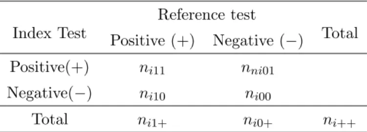
When the reference test can be considered as a gold standard, letnitddenote the number of subjects with index test results T = t and disease status Dis = d for study i (i = 1,2, . . . , N), wheretanddare defined in Chapter 1. Thus,ni11,ni00,ni01, andni10 are the number of true positives, true negatives, false positives and false negatives for theith study, respectively. Let ni1+ =ni11+ni10 and ni0+ =ni01+ni00 be the study-specific numbers of diseased and disease-free subjects. Then the study-specific sensitivity and specificity can be estimated as dSei =ni11/ni1+, and dSpi =ni00/ni0+. See Table 2.1 for
Table 2.1: 2 by 2 table for ith study Reference test
Index Test Positive (+) Negative (−) Total
Positive(+) ni11 nni01
Negative(−) ni10 ni00
Total ni1+ ni0+ ni++
a typical 2 by 2 table for study i.
In this section, we will first discuss the conventional summary receiver operating characteristic (ROC) approach and a bivariate approach using linear mixed models (LMM). Both methods require direct calculations of study-specific sensitivities and specificities, and an ad hoc continuity correction when there are zero events in either arm of a study. Second, we will discuss the hierarchical summary ROC approach for jointly modeling positivity criteria and accuracy parameters, and a bivariate approach using GLMM for jointly modeling sensitivities and specificities. At last, we will discuss a trivariate approach using GLMM for jointly modeling prevalence, sensitivities and specificities to assess the correlations among the three parameters. The hierarchical summary ROC approach, and the bivariate and trivariate approaches are based on the exact binomial distribution and thus do not require any ad hoc continuity correction. [43]
2.1.1 The summary ROC method
The summary ROC curve method was first proposed by Moses et al. [54]. Reflecting the trade-off between sensitivity and specificity caused by implicit thresholds, this method has been widely used in diagnostic tests studies. The observed Se and Sp estimates form a concave ROC curve shape as the threshold varies. Such curve can be fitted by back-transforming the linear relationship between logit transformations of Se and Sp to the ROC space: First, if some studies have ni11 = 0 or ni00 = 0, an ad hoc continuity correction is applied by adding 0.5 to each of the 4 cells of such studies. After the correction, sensitivity is estimated to be dSei = (ni11+ 0.5)/(ni1++ 1) and specificity is
12 S and Das the sum and the difference of logit transformed sensitivity and specificity, such that Si= logit(dSei) + logit(dSpi) andDi = logit(dSei)−logit(Spdi), where logit(p) =
log{p/(1−p)}, 0 < p < 1. (This notation is slightly different than Moses et al.[54] because the original transformation is on Se and false positive rate (FPR, equivalent to 1-Sp)). One can see that Si = log(ORdi), where ORdi = nni11
i10
ni01
ni00 is the diagnostic odds
ratio for the ith study. Third, for N studies, fit a linear regression line S = a+bD either by an ordinary least squares or by a weighted least squares method weighing by the inverse of within-study variances var(log(ORi))−1, where var(log(ORi)) = 1/ni11+ 1/ni10+ 1/ni01+ 1/ni00 [4]. After fitting the regression line using either method, one can plot the summary ROC curve by the two estimated coefficients (i.e., intercept ˆa and slope ˆb),
Se={1 +e−ˆa/(1−ˆb)× Sp/(1−Sp)(1+ˆb)/(1−ˆb)
}−1, (2.1)
with Se on the y-axis and 1−Sp on the x-axis. To adjust for study-level covariates
Z (e.g., different sites the diagnostic tests were taken), one can fit a model with Si = a+bDi+cZi. We can then haveSi = ˆa+ ˆbDi+ ˆcZi= (ˆa+ ˆcZi) + ˆbDi= ˆa0+ ˆb0Di. The summary ROC curve can be plotted according to new estimates ˆa0 and ˆb0 given Z.
The summary ROC method is easy to perform but suffers some shortcomings. On the one hand, its interpretations are known to be problematic. Walter discussed the in-terpretation of area under the curve (AUC) [17]. A summary ROC curve located closer to the left upper corner of the ROC space will have a larger AUC, indicating better predictive accuracy of a test [17]. However, the conclusion becomes unreliable when comparing tests whose summary ROC curves may cross each other. Alternative statis-tics, such as the partial AUC [55] and the Q point [56] also have limited applications. On the other hand, the model setting has some drawbacks. First, because Si = log(ORdi),
the data are reduced to one outcome measure per study: diagnostic odds ratio. In-dependent summaries of sensitivity and specificity are not available, which could be important in test evaluating. Second, the model is restricted in that the between-study heterogeneity can only be adjusted by study level covariates, such that some compo-nents of the variance might not be explained. This is the reason why both Moses et al.[54] and Irwig et al. [57] recommended the unweighted least squares rather than the weighted as in a fixed effect model as a few large studies may dominate the result if
the between-study variation is present. Third, in practice, study characteristics besides the cut-point effect contribute to the trade-off between sensitivity and specificity within a study[54, 58], which are not incorporated in the summary ROC curves. Finally, an arbitrary continuity correction is needed to handle zero cells. Moses showed that it can push the summary ROC curve far from the ideal upper left corner of the ROC space, giving biased results [55].
2.1.2 A bivariate approach based on LMM
To improve over the summary ROC method, Reitsma et al. proposed a bivariate LMM [11]. The model proceeds as follows. First, a logit transform of the sensitivity and specificity is applied to each study. Different from the summary ROC method, they are considered as random by allowing variation according to normal distributions, that is logit(Sei) ∼ N(α, σµ2) and logit(Spi) ∼ N(β, σν2) . A bivariate normal distribu-tion can include possible correladistribu-tion between sensitivity and specificity within study:
logit(Sei) logit(Spi) ! ∼ N α β ! ,Σ ! , where Σ = σ 2 µ σµν σµν σ2ν !
and σµν denotes the
covariance between logit sensitivity and specificity.
Second, to account for the sampling variation, the estimated logit sensitivity and
specificity are assumed to be normally distributed as logit(dSei) logit(Spdi) ! ∼N logit(Sei) logit(Spi) ! , Ci !
for study i, with Ci =
var(logit(dSei)) 0
0 var(logit(dSpi)) !
, var(logit(dSei)) = 1/ni11+
1/ni10 and var(logit(dSpi)) = 1/ni10+ 1/ni00. Note that, the general rule that ni1+dSei,
ni1+(1−dSei), ni0+Spdi and ni0+(1−Spdi) are at least five need to hold for normal
ap-proximation to be valid. Consequently, logit(dSei) and logit(dSpi) are assumed to have
the following bivariate normal distribution:
logit(dSei) logit(dSpi) ! ∼N α β ! ,Σ+Ci ! (2.2)
Because the distributions of sensitivity and specificity are often skewed, one may prefer inference based on the medians rather than means as the overall diagnostic test perfor-mance summary. Based on parameter estimates, the median sensitivity and specificity can be back-transformed asSe[M = logit−1(αb) andSp[M = logit
−1(
b
14 the inverse logit function such that logit−1(x) = 1/(1 + exp(−x)). Similarly, confidence intervals forSe[M andSp[M can be transformed from the confidence intervals of ˆαandβb.
The correlation between sensitivity and specificity can be estimated as σˆµν ˆ
σµ×σˆν. The stan-dard errors are SE(Se[M) = SE(α)
1/Se[M+1/(1−Se[M)
and SE(Sp[M) = SE(β) 1/Sp[M+1/(1−Sp[M)
based on the Delta method. A summary ROC curve can be constructed by the regression of logit sensitivity over given specificity as
logit(Se) = ˆα+ ˆσµν ˆ σ2 ν logit(Sp)−βˆ. (2.3)
In general, this approach is superior to the summary ROC model by analyzing sensitivity and specificity jointly in a bivariate LMM (BLMM). However, the bivariate approach estimates the degree of correlation between sensitivity and specificity, as well as both within- and between-study variation in the two indicators separately. A drawback of this approach is that an ad hoc continuity correction is required in the presence of zero cells, as with the summary ROC approach. In addition, the general rule of normal approximation is sometimes violated in practice[10]. The bivariate model can adjust for covariates by regression model in the mean vector of the bivariate normal distribution:
logit(Sei) logit(Spi) ! ∼N α+γZi β+λZi ! ,Σ !
, where Zi is the study-level covariate andγ,
λare the corresponding coefficient parameters [4].
2.1.3 The hierarchical summary ROC approach
Rutter and Gatsonis proposed a hierarchical summary ROC approach[2], which is a simplification of the ordinal regression model by Tosteson and Begg: g(γj(x)) = (θj −
α0x)eβ0x, whereg(·) is a link function,γj(x) is the probability of a response being in one of the ordered categories given covariates x,θj is the cutoff values of each category, α is the location parameters and βis the scale parameter[59]. The hierarchical summary ROC approach reduces the ordinal regression model to two categories (j = 1,2), x
indicates true disease status (coded as 0.5 for Dis= 1 and−0.5 forDis= 0) andγj(x) correspond to positive test rates: Sei and 1−Spi (FPR)[2].
The first stage assumes binomial distributions of the number of positive outcomes in the ith study, i.e., ni11 ∼Bin(ni1+, Sei) and ni01 ∼Bin(ni0+,1−Spi). Choose g(·)
to be logit link, the model is written as
logit(Sei) = (θi+ 0.5αi)e−0.5β,logit(1−Spi) = (θi−0.5αi)e0.5β, (2.4) where the latter is the same as logit(Spi) =−(θi−0.5αi)e0.5β. The positivity criteriaθi model the tradeoff between sensitivity and specificity in each study. Direct interpreta-tions of the accuracy parametersαi are that whenβ = 0,αi = logit(Sei) + logit(Spi) = log(ORi), which is independent ofθi. In the second stage, Rutter and Gatsonis allow θi and αi to vary across studies[2]. Thus, θi and αi are assumed independently normally
distributed as: θi αi ! ∼N θ0 α0 ! , σ 2 θ 0 0 σ2 α !! .
A summary ROC curve can be derived based on solving functions in (2.4) as
logit(Sei) =αie−β/2+e−βlogit(1−Spi)
Another possible construction of summary ROC curve pointed out by Chu et al.[12] is based on the bivariate normal distribution of θi and αi and the Delta method as
logit(Se) =e−0.5 ˆβ(0.5 ˆα0+ ˆθ0)+
0.25ˆσα2 −σˆ2θ 0.25ˆσ2
α+ ˆσ2θ
×e−βˆ{logit(Sp)−e−0.5 ˆβ(0.5 ˆα0−θˆ0)}. (2.5) In addition, Arends et al. discussed several choices of SROC curves[9]. Median sen-sitivity and specificity estimates are Se[M =
n 1 +exp{−(ˆθ0 + 0.5 ˆα)e−0.5 ˆβ} o−1 and [ SpM = n
1 +exp{(ˆθ0 −0.5 ˆα)e0.5 ˆβ}o−1. Also, similar as the previous model, the hier-archical summary ROC approach can incorporate study level covariates by θi
αi ! ∼ N θ0+γZi α0+λZi ! , σ 2 θ 0 0 σα2 !! .
The hierarchical summary ROC approach incorporates both within- and between-study variability and the correlation between the summary statistics by random effects θi and αi. Because sparse data is common in meta-analysis of diagnostic tests, espe-cially under low event rates, an important advantage over the previous models is that the hierarchical summary ROC approach avoids the continuity correction by assuming binomial distributions[2]. A practical limitation of this model is that originally it is fitted via Bayesian Markov Chain Monte Carlo approach using BUGS, which requires some level of programming skills. This approach is found to be the same as the following bivariate GLMM with alternative parameterizations in some situations.
16
2.1.4 The bivariate generalized linear mixed model (GLMM)
Chu and Cole presented a bivariate GLMM to jointly analyze sensitivity and specificity using logit link[10]. Later, the bivariate GLMM was adjusted to a general link function [45]. The model starts with binomial distribution assumptions and applies link functions on the probability parameters:
ni11∼Bin(ni1+, Sei), ni00∼Bin(ni0+, Spi), g(Sei) =α+µi, g(Spi) =β+νi, (2.6) where µi and νi are random effects follow bivariate normal distribution
µi νi ! ∼ N 0 0 ! , σ 2 µ ρµνσµσν ρµνσµσν σ2ν !!
, and g(·) is a link function such as the logit, probit, and complimentary log-log link. Different link functions can be applied to sensitivity and specificity separately. Though logit link is widely used in meta-analysis to date, Chu et al. argued that, for some meta-analyses, the choice of the link may affect model fit and inference[45]. The parametersσµ2 andσ2ν estimate the between-study variances and ρµν explain possible correlations.
The model gives median estimates as Se[M = logit−1( ˆα) and Sp[M = logit−1( ˆβ). Similarly, confidence intervals forSe[M andSp[M can be transformed from the confidence intervals of ˆα and ˆβ. Study-level covariateZ can be adjusted byg(Sei) =α+µi+γZi andg(Spi) =β+νi+λZi, whereγ,λare corresponding coefficient parameters. Different covariates could be adjusted for sensitivity and specificity. A regression line of g(Se) on g(Sp),g(Se) = ˆα+ ˆρµνσσˆˆµν[g(Sp)−βˆ], gives the summary ROC curve by transforming to the ROC space. Also, alternative choices of the regression lines can construct different summary ROC curves with corresponding interpretations[9].
In addition to estimating the heterogeneity and correlation parameters, both hi-erarchical summary ROC and bivariate GLMM approaches have advantages over the bivariate LMM. First, the bivariate GLMM does not require the general rule of nor-mal approximation to estimate var(logit(Seci)) and var(logit(Spci)). Second, neither the
two approaches require continuity correction because direct calculation of study-specific sensitivities and specificities is not involved. In the absence of study-level covariates, the two approaches are the same model with alternative parameterizations[5].
Both hierarchical summary ROC and bivariate GLMM can be fitted using the max-imum likelihood approach. Several numerical methods might be used, for instance,
the dual quasi-Newton optimization techniques, as implemented in SAS NLMIXED procedure. The standard errors and confidence intervals for interested parameters are estimated by the Delta method and are reported if specified in the ESTIMATE state-ment. To restrict the correlation coefficient ρµν in the range [-1, 1] in the bivariate GLMM, one can use the Fisher’s z transformation of ρµν in programming. AUC for both hierarchical summary ROC and bivariate GLMM can be computed by numerical integration implemented in SAS macro.
2.1.5 The trivariate GLMM
The above approaches involving only sensitivities and specificities work best if all or the majority of the studies use case-control designs with non-identifiable prevalence. When disease prevalence estimation is allowed in cohort study designs, we can derive other clinically interested indices such as positive and negative predictive values (PPV and NPV) by estimates of sensitivity, specificity and prevalence. In this case, a challenge is the potential dependence of test performance on prevalence, which can be termed spectrum bias[26]. Typically, such dependence is mostly concerned when the bivariate diagnostic outcome is based on the cut point on continuous traits, thus misclassification rates could be higher among subjects with true value around the cut point[60]. To account for this potential dependence, Chu et al. extended the bivariate GLMM to a trivariate GLMM jointly modeling the disease prevalence, sensitivity and specificity[16]. Recently, Li and Fine proposed a Pearson type correlation coefficient to assess this dependence by an estimating equation-based regression framework[61].
Here, we only consider a trivariate GLMM based on the parameterization ofπi,Sei and Spi, where πi is the disease prevalence in ith study. The first level of this model assumes binomial distributions:
ni1+ ∼Bin(ni++, πi), ni11∼Bin(ni1+, Sei), ni00∼Bin(ni0+, Spi). (2.7) The parameters are modeled via link functions: g(πi) = η+εi, g(Sei) = α+µi and g(Spi) =β+νi. See Table 2.2 a two by two table accounting for disease prevalence.
18
Table 2.2: 2 by 2 table forith study accounting for prevalence Reference test
Index Test Positive (+) Negative (−) Total
ni11 nni01 Positive(+) π iSei (1−πi)(1−Spi) ni10 ni00 Negative(−) π i(1−Sei) (1−πi)Spi ni1+ ni0+ ni++ Total π i 1−πi 1
and νi are assumed to be random effects with trivariate normal distribution:
εi µi νi ∼N 0 0 0 ,Σ , where Σ = σ2ε ρεµσµσε ρενσνσε σ2µ ρµνσµσν σ2ν
The parameters σε2, σµ2 and σ2ν capture the between-study variance of the disease prevalence, sensitivity and specificity while ρεµ,ρεν and ρµν represent correlations.
Standard software such as SAS NLMIXED can maximize the likelihood. To avoid including unnecessary parameters, model selection criteria such as Akaike information criterion (AIC) can be used. By parameter estimates, the medians are derived as πcM = g−1(ˆη),Se[M =g−1( ˆα) andSp[M =g−1( ˆβ). In this model, covariates can be incorporated in sensitivities, specificities and disease prevalence as was done for the bivariate GLMM.
2.2
Statistical methods when the reference test is not a
gold standard
Limited meta-analysis tools are available when the reference test is imperfect. Walter et al. discussed the latent class model for a meta-analysis of two diagnostic tests[17]. Sadatsafavi et al. presented a latent class random effects model[19]. However, other than prevalence, only one of the sensitivity and specificity can be implemented as a random effect. Dendukuri et al. presented a Bayesian approach, which is an extension of the hierarchical summary ROC model, to adjust for different reference standards[20].
We hereby introduce the latent class random effects model by Chu et al. using random effects to allow variation and correlation in sensitivity, specificity and prevalence between studies[18].
Let (SeBi, SpBi) be the pair of diagnostic accuracy parameters for the reference test while (SeAi, SpAi) be the pair for the index test. To construct the 2 by 2 table (Table 2.3) for such studies, both the above pairs of statistics and the disease prevalence are needed.
20 Table 2.3: 2 by 2 table when the reference test is not a gold standard
Reference test
Index Test Positive (+) Negative (−) Total
ni11 ni01 Positive(+) p i11=πiSeAiSeBi+ (1−πi)(1−SpAi)(1−SpBi) pi01=πiSeAi(1−SeBi) + (1−πi)(1−SpAi)SpBi ni10 ni00 Negative(−) p i10=πi(1−SeAi)SeBi+ (1−πi)SpAi(1−SpBi) pi00=πi(1−SeAi)(1−SeBi) + (1−πi)SpAiSpBi ni1+ ni0+ ni++ Total p i1+=πiSeBi+ (1−πi)(1−SpBi) pi0+=πi(1−SeBi) + (1−πi)SpBi 1
The four counts in Table 2.3 follow a multinomial distribution, with log-likelihood being:
logL=X i
{ni11log(pi11) +ni10log(pi10) +ni01log(pi01) +ni00log(pi00)}. (2.8) Chu et al. used random effects to model between and with-in study heterogeneity and potential correlations[18]. We write this model in a form suit for a general link functiong():
g(πi) =η+εi;g(SeAi) =αA+µAi;g(SpAi) =βA+νAi;
g(SeBi) =αB+µBi;g(SpBi) =βB+νBi
where random effects follow a multivariate normal distribution: (εi, µAi, νAi, µBi, νBi)0 ∼ N(0,Σ) with variance-covariance matrix
Σ= σ2ε ρεµAσεσµA ρενAσεσνA ρεµBσεσµB ρενBσεσνB σ2 µA ρµAνAσµAσνA ρµAµBσµAσµB ρµAνBσµAσνB σν2A ρνAµBσνAσµB ρνAνBσνAσνB σµ2B ρµBνBσµBσνB σ2νB
Median estimates of prevalence, sensitivities and specificities can be achieved by
c
πM = g−1(ηb), Se\AM = g
−1(
c
αA), Sp\AM = g−1(βcA), Se\BM = g−1(αcB) and Sp\BM =
g−1(βcB). Variance and correlation parameter estimates can be derived from Σb.
Co-variates Z can be adjusted by linear regressions in the mean vectors, for instance g(πi) =η+εi+γZi.
This latent class random effects model fills in the gap of models for meta-analysis of diagnostic test under imperfect reference test condition. It can evaluate the performance of both the diagnostic test of interest and the reference test while keep all the advantages of the GLMMs. A limitation applies when fitting this model by SAS NLMIXED. One could encounter convergence problem because of limited number of studies and relatively large number of parameters. Possible simplifying assumption could be independence of disease prevalence against the other parameters. Also, to avoid including redundant random effects whose variance approximates zero, one can apply a forward selection based on AIC.
22
2.3
Discussion
In this chapter, we discussed the methods for evaluating the performance of diagnostic tests for situations when the reference test can be considered a gold standard, as well as situations when it is error-prone. Under the scenario with gold standard, we reviewed the traditional summary ROC method, bivariate LMM and the hierarchical summary ROC model. Then we focused on the random effect GLMM, because it has several advantages over simpler methods. In this section, we showed how the bivariate GLMM can be fitted using different link functions other than logit link, and extended the approach to a trivariate GLMM to model prevalence as well as sensitivity and specificity. Under the situation with no gold standard, we built upon the latent class model proposed by Walter et al.[17] by adding random effects to quantify possible correlation and variation following the method by Chu et al.[18].
Among the models presented, the summary ROC approach is simple and widely used, while receives a number of critical comments on problems related to the interpretation of summary ROC curves, the fixed effects model and the continuity correction. The bivariate LMM improves over the summary ROC approach by assuming random effects to explain both within- and between study variations and possible correlation. The bivariate LMM can give inferences both in terms of summary ROC curves and summary statistics of overall test performance. However, it has some limitations due to the continuity correction and the validity of normal approximation. The GLMMs do not have the limitations of the above models by assuming exact binomial distributions. The bivariate GLMM, which is essentially the same as the hierarchical summary ROC model in some situations, can be used when the majority of the studies use case-control designs and the trivariate GLMM can be used when most of the studies are cohort studies.
A limitation related to the GLMMs is that the meta-analysis reported often includes a mixture of case-control and cohort studies designs. Thus using either the bivariate or the trivariate GLMM for all the studies can lead to some issues. Another problem arises when fitting the trivariate GLMM and the latent class random effects models in SAS procedure NLMIXED. The more random effects included, the longer it took to converge. Under such situations, one can first get raw estimates of the desired parameters by fitting the data in models with less random effects. The raw estimates can then be used to
adjust the initial values to improve convergence. For the latent class random effects model, one may need to apply simpler assumptions for ease of fitting.
Chapter 3
A hybrid Bayesian hierarchical
model combining cohort and
case-control studies for
meta-analysis of diagnostic tests:
Accounting for partial verification
bias
As discussed in the previous Chapter, many meta-analyses of diagnostic tests in practice contain both cohort and case-control study designs [23]. However, the trivariate GLMM [16] can only include cohort studies with information estimating study-specific disease prevalence and the bivaraite GLMM cannot estimate prevalence and account for the correlation between prevalence and accuracy parameters. On the other hand, some diagnostic accuracy studies only select a subset of samples to be verified by the reference test. It is known that ignoring unverified subjects may lead to partial verification bias in the estimation of prevalence, sensitivities, and specificities in a single study [31]. However, the impact of this bias on a meta-analysis has not been investigated. In this chapter, we propose a novel hybrid Bayesian hierarchical model combining cohort and
casecontrol studies and correcting partial verification bias at the same time. We first describe the proposed method in Section 3.1. We investigate the performance of the proposed methods through a set of simulation studies in Section 3.2. Section 3.3 provides two motivating case studies: assessing the diagnostic accuracy of gadolinium-enhanced magnetic resonance imaging (MRI) in detecting lymph node metastases and of adrenal fluorine-18 fluorodeoxyglucose positron emission tomography (PET) in characterizing adrenal masses. This chapter ends with a discussion in Section 3.4. The data sets for the two case studies are given in Appendix A.
3.1
Bayesian hierarchical model
3.1.1 Notations
Suppose that we have a meta-analysis with N diagnostic accuracy studies, and the studies are indexed such that theN1cohort studies come first, followed byN2 =N−N1 case-control studies. To allow partial verification in some of the first N1 cohort studies, let nitd be the number of subjects with disease status Dis = dand test results T =t (d, t= 0,1, mindicating negative, positive and missing results, respectively) in the ith study (i= 1,2, . . . , N1) andpitd be the corresponding probability. As subjects with both DisandT missing do not provide any information, we will not consider them. Defineπi, Sei andSpi as in previous chapters. LetV = 1 andV = 0 denote the subject is verified or not, respectively. Let ωitm (t= 0,1) and ωimd (d= 0,1) be the mutually exclusive probabilities of missing for subjects with test result T =t and disease statusDis =d, respectively. Furthermore, given the nature of case-control studies, it is unnecessary to consider the influence of missing data in case-control studies: subjects with unverified disease status generally do not exist and subjects with missing diagnostic test outcomes can be ignored as prevalences in such studies are not well defined.
Table 3.1 presents the data structure and notation for the ith study when it is a cohort study or a case-control study. In each cell, the number of cell counts and the corresponding probabilities are presented. The left panel is for a cohort studies, which extends a standard 2×2 table (Table 2.2) to allow for partial verification. The sum of all cell probabilities is one. The right half is for a case-control studies with a typical
26 2×2 table (Table 2.1). The cell probabilities sum up to one for diseased and non-diseased subjects separately. Derivations of the cell probabilities for cohort studies are also provided at the footnote of Table 3.1 .
27 Gold standard
Cohort (i= 1, . . . , N1) Case-control (i=N1+ 1, . . . , N)
Index test + − Missing + −
+ ni11 ni10 ni1m ni11 ni10 (1−ωi1m−ωim1)πiSei (1−ωi1m−ωim0)(1−πi)(1−Spi) ωi1m{πiSei+ (1−πi)(1−Spi)} Sei 1−Spi − ni01 ni00 ni0m ni01 ni00 (1−ωi0m−ωim1)πi(1−Sei) (1−ωi0m−ωim0)(1−πi)Spi ωi0m{πi(1−Sei) + (1−πi)Spi} 1−Sei Spi Missing nim1 nim0 ωim1πi ωim0(1−πi)
In each cell, the number of cell counts are presented and the probabilities corresponding to the cell counts are presented below the cell counts.
Probabilities for subjects withV = 1 in theith cohort study:
pi11=P(V = 1|Dis= 1, T = 1)P(Dis= 1)P(T = 1|Dis= 1) = (1−ωi1m−ωim1)πiSei,
pi10=P(V = 1|Dis= 0, T = 1)P(Dis= 0)P(T = 1|Dis= 0) = (1−ωi1m−ωim1)(1−πi)(1−Spi), pi01=P(V = 1|Dis= 1, T = 0)P(Dis= 1)P(T = 0|Dis= 1) = (1−ωi0m−ωim1)πi(1−Sei), pi00=P(T = 0|Dis= 0)P(V = 1|Dis= 0, T = 0)P(Dis= 0) = (1−ωi0m−ωim0)(1−πi)Spi. Probabilities for subjects withV = 0 in theith cohort study:
pi1m = P(V = 0|T = 1)P(T = 1) = P(V = 0|T = 1){P(T = 1, Dis= 1) +P(T = 1, Dis= 0)} =P(V = 0|T = 1){P(Dis= 1)P(T = 1|Dis= 1) +P(Dis= 0)P(T = 1|Dis= 0)}=ωi1m{πiSei+ (1−πi)(1−Spi)},
pi0m = P(V = 0|T = 0)P(T = 0) = P(V = 0|T = 0){P(T = 0, Dis= 1) +P(T = 0, Dis= 0)} =P(V = 0|T = 0){P(Dis= 1)P(T = 0|Dis= 1) +P(Dis= 0)P(T = 0|Dis= 0)}=ωi0m{πi(1−Sei) + (1−πi)Spi},
28
3.1.2 The likelihood with random effects accounting for heterogeneity
Letω={ωi}and θ={θi}, whereωi= (ωi0m, ωi1m, ωim0, ωim1) andθi = (πi, Sei, Spi) for study i. Assuming independence among subjects conditional on θi and ωi, the likelihood is the product of contribution from each study. Multinomial likelihoods are used for cohort studies and binomial likelihoods are used for case-control studies. In this paper we assume verification is MAR, where the missing probabilitiesωare independent of prevalence and test accuracy parameters,θ. Therefore, the likelihood can be factored asL(θ,ω|Data)∝L(θ|Data)×L(ω|Data). Specifically,
L(ω|Data)∝ N1 Y i=1 ωni1m i1m ω nim1 im1 ω nim0 im0 ω ni0m i0m Y j,k=0,1
(1−ωijm−ωimk)nijk
(3.1) and L(θ|Data)∝ N Y i=1 Seni11 i (1−Spi)ni10(1−Sei)ni01Spnii00 N1 Y i=1 πi P j nij1 (1−πi) P j nij0 hni1m i1 h ni0m i0 , (3.2) where hi1 =πiSei+ (1−πi)(1−Spi),hi0=πi(1−Sei) + (1−πi)Spi andj = 0,1, m.
To account for potential between-study heterogeneity, we consider a GLMM:
g(πi) =η+εi; g(Sei) =α+µi; g(Spi) =β+νi, (3.3)
where g() is a link function, and (εi, µi, νi)T is a random effect vector. To account for potential correlation among πi, Sei and Spi, (εi, µi, νi)T is assumed to be multivariate normally distributed as (εi, µi, νi)T ∼N(0,Σ), where
Σ= σε2 ρεµσµσε ρενσνσε σ2 µ ρµνσνσµ σν2 .
The diagonal of the variance-covariance matrixΣ, (σ2ε, σµ2, σν2), characterize the between-study heterogeneity of disease prevalence, test sensitivities and specificities, while the parameters (ρεµ, ρεν, ρµν) capture the correlations between the corresponding random ef-fects (πi, Sei), (πi, Spi) and (Sei, Spi) in transformed scale, respectively. For simplicity, we assume the same correlation structure for sensitivities, specificities and prevalences for both case-control and cohort studies in this paper, which can be easily relaxed if
necessary. However, for case-control studies, the study-specific prevalences are not con-tained in the likelihood and not directly estimable, and can be predicted using this correlation structure and study-specific sensitivity and specificity.
Study-level covariates, such as study quality, type of design (case-control versus cohort studies), race distribution and mean age, can be incorporated through meta-regression when necessary. For example, let g(πi) = η0 +η1Xi+εi, g(Sei) = α0 +
α1Wi +µi and g(Spi) = β0+β1Zi +νi, where Xi, Wi and Zi denote the possibly overlapping study-level covariate vectors. Note that the hybrid GLMM accounts for different study designs in the construction of likelihood. Including type of study design as a covariate is helpful when there is a systematic difference between cohort and case-control studies, e. g., if the pooled sensitivity and specificity are believed to be different between the two designs.
The marginal likelihood integrated over random effects is:
L(θ,ω) =
Z Z Z
L(θ,ω|Data)×p(µi, νi, εi|Σ)dεidµidνi (3.4) Frequentist methods (such as the maximum likelihood estimate) may converge slowly or have convergence problems due to the need to maximize the marginal likelihood with trivariate integrations, and the corresponding asymptotic approximations for standard errors of functions of parameters may not be sufficiently accurate [44].
3.1.3 Bayesian posterior sampling approach
In this chapter, we consider fully Bayesian approaches using Markov chain Monte Carlo (MCMC) methods for parameter estimation. In most instances, inferences obtained by Bayesian and classical frequentist methods are similar when the former uses non-informative or weakly non-informative prior distributions for all model parameters [62]. Compared to the frequentist methods, MCMC algorithms permit full posterior inference (e.g., credible intervals) even when the normality approximation based on large sample theory is insufficient, which is valuable here because the sampling distributions of π, Se, Sp, PPV, NPV, LR+ and LR− are often skewed and the number of studies in the meta-analysis is relatively small or moderate (e.g., N < 30). Specifically, we will draw posterior inference using Gibbs and Metropolis-Hastings sampling algorithms [63,
30 64, 65, 66] with convergence assessed using trace plots, sample autocorrelations, and statistical convergence diagnostic tests [67, 68].
Letp(η), p(α),p(β) and p(Σ) denote the prior distributions for η,α,β and Σ. We take non-informative normal priors on η, α, β and a Wishart prior on the precision matrix Σ−1 (inverse Wishart prior onΣ), denoted by
p(η)∼N(0,102); p(α)∼N(0,102); p(β)∼N(0,102); p(Σ−1)∼W(R, v), (3.5) where R is a 3 by 3 matrix, and a small number is chosen as the degrees of freedom v (v≥3). The posterior distribution of η, α, β and Σcan be written as:
p(η, α, β,Σ|Data)∝L(θ|Data)p(η)p(α)p(β)p(Σ) N
Y
i=1
p(εi, µi, νi|Σ) (3.6) where L(θ|data) depends on (η, α, β) through πi =g−1(η+εi), Sei=g−1(α+µi) and Spi = g−1(β +νi), and g−1(·) is the inverse function of the link function g(·). When study-level covariates are included in the link functions, plug inπi =g−1(η0+η1Xi+εi), Sei =g−1(α0+α1Wi+µi) andSpi=g−1(β0+β1Zi+νi) instead. Here we focus on the model without covariates for simplicity of the presentation.
Using the MCMC samples of η, α, and β, the posterior samples for population-averaged PPV, NPV, LR+, LR−can be approximated by the following formulas:
P P V = g −1(η)g−1(α) g−1(η)g−1(α) +{1−g−1(η)}{1−g−1(β)} N P V = {1−g −1(η)}g−1(β) {1−g−1(η)}g−1(β) +g−1(η){1−g−1(α)} LR+ =g−1(α)/{1−g−1(β)}, LR−={1−g−1(α)}/g−1(β)
3.2
Simulation
3.2.1 Simulation designWe conduct 12 sets of simulations to compare the proposed Bayesian hybrid GLMM (3.1) to two alternative approaches which researchers are likely to apply in practice: 1) a complete case analysis approach in which subjects not verified are ignored (model 3.2); and 2) a trivariate GLMM approach in which case-control studies are excluded from the
analysis (model 3.3). To fit model 3.2, case-control and cohort studies are combined as in the hybrid GLMM, while the missing counts are excluded. To fit model 3.3, the missing counts are accounted for as in the hybrid GLMM, while all case-control studies are excluded from the data. To investigate the performance of the proposed hybrid GLMM, for each generated dataset, we fit the hybrid GLMM, model 3.2 and model 3.3 separately using R package BRugs [69]. Each dataset contains equal numbers of case-control and cohort studies, where cohort studies are subject to partial verification. The probabilities of missing a reference test are 0.2 and 0.8, given diagnostic test results being positive and negative, respectively. The median prevalence is set to be 0.2 with the variances asσ2
ε = σ2µ=σν2 = 1, and the number of subjects per study is chosen to be similar to the case studies in Section 3.3. Specifically, we consider 12 settings with small (10) or moderate (30) number of studies in a meta-analysis and high sensitivity (specificity) as 0.9 (0.95), or low sensitivity (specificity) as 0.7 (0.8), respectively. To evaluate the impact of the correlation structure, the correlation parameters (ρεµ, ρεν, ρµν) are chosen as (0, 0, 0), (0.5, −0.5, −0.5) or (0.8, −0.8, −0.8) to correspond to no correlation, moderate or strong correlations among disease prevalence and test sensitivity and specificity (in logit scale). We assume a positive correlation between πi and Sei as it is likely to happen when population with higher prevalence may have more patients with clear-cut disease condition, leading to a higher sensitivity. However, a negative correlation was also observed in some studies[21]. For each setting, 2000 replicates are generated using the trivariate logit-normal random effects model. The posterior statistics (median and 95% equal tailed credible interval) are summarized from 10000 posterior samples with 5000 burn-in iterations. Model performance