ARISTOTELIS PANAGIOTOPOULOS AND S LAWOMIR SOLECKI
Abstract. We represent the universal Menger curve as the topological real-ization|M|of the projective Fra¨ıss´e limitMof the class of all finite connected
graphs. We show that M satisfies combinatorial analogues of the Mayer–
Oversteegen–Tymchatyn homogeneity theorem and the Anderson–Wilson pro-jective universality theorem. Our arguments involve only 0-dimensional topol-ogy and constructions on finite graphs. Using the topological realization
M7→ |M|, we transfer some of these properties to the Menger curve: we prove
the approximate projective homogeneity theorem, recover Anderson’s finite ho-mogeneity theorem, and prove a variant of Anderson–Wilson’s theorem. The finite homogeneity theorem is the first instance of an “injective” homogeneity theorem being proved using the projective Fra¨ıss´e method. We indicate how our approach to the Menger curve may extend to higher dimensions.
Introduction
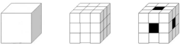
The Menger curve is a 1-dimensional Peano continuum that is classically ex-tracted from the cube in the same way that the Cantor space is exex-tracted from the interval: subdivide C0 = [0,1]3 into 33 congruent subcubes; let C1 be the union
of these subcubes which intersect the one-skeleton of [0,1]3; repeat this process
on each subcube again and again to define Cn; the Menger curve is defined to be the intersectionT
nCn. With this construction Menger found the first example of
a universal space for the class of 1-dimensional continua, that is, a 1-dimensional continuum in which every other 1-dimensional continuum embeds [14].
Figure 1. FromC0 toC1.
The Menger curve is a canonical continuum whose topological properties do not depend on the various geometric parameters of the above iterative process. In fact, many other constructions of universal 1-dimensional continua (e.g., [12, 16]) which appeared soon after [14] were later shown to produce the same space; see [1].
2010Mathematics Subject Classification. 03C30, 54F15.
Key words and phrases. Projective Fra¨ıss´e limits, Menger curve, homogeneity, universality, homology Menger compactum.
Research of Solecki supported by NSF grants DMS-1800680 and 1700426.
In this paper, we develop a combinatorial model for the Menger curve using an analogue of projective Fra¨ıss´e theory from [10]. The Menger prespace M is a compact graph-structure on the Cantor space. In a sense,Mis thegeneric inverse limit in the category C of all connected epimorphisms between finite connected graphs. The edge relation on M turns out to be an equivalence relation and the
Menger curve is then defined to be the quotient|M|=M/RofM with respect to this relation.
This definition of the Menger curve as the topological realization |M| of the
combinatorial objectMhas certain technical and foundational advantages. On the foundational side, the definition ofMis canonical since it is constructed throughC without making any ad-hoc choices for the bonding maps. Moreover, the definition of |M| is intrinsic, in that it makes no reference to external spaces such as such
as [0,1]3. On the technical side, when proving results about the Menger curve,
we can often replace various complications coming from 1-dimensional topology of |M| with combinatorial problems about graphs in C. Moreover, like any other
projective Fra¨ıss´e limit,Mhas the following projective extension property built in
by the construction: for everyg ∈ C and any connected epimorphism f as in the diagram, there is a connected epimorphismhwithg◦h=f.
M A
B h
f
g
Having this universal property ofMas our point of departure, and expanding on it using combinatorial properties ofC, we can integrate various aspects of the Menger curve into a unified theory as follows.
• Anderson’s homogeneity theorem [1] states that any bijection between finite subsets of|M|extends to a global homeomorphism of|M|. This theorem was
later generalized in [13] to the strongest possible homogeneity result for|M|,
namely, that every homeomorphism between locally non-separating, closed subsets of|M|extends to a global homeomorphism of|M|. In Theorem 4.1,
we prove a homogeneity result forM analogous to the homogeneity result
for the Menger curve in [13]. From that we recover Anderson’s homogeneity result for|M|. Our proof of Theorem 4.1 relies onC being closed under a certain mapping cylinder construction.
• Anderson–Wilson’s projective universality theorem states that|M|admits
an open, continuous, and connected map onto any Peano continuum1.
Moreover, all preimages of points under this map can be taken to be home-omorphic to the Menger curve [2, 20]. In Theorem 5.1, we prove a combi-natorial analogue of the Anderson–Wilson theorem for M. In the process, we isolate a combinatorial property ofC that is responsible for this strong form of projective universality. In Corollary 5.1, we establish a variant
1In this paper we use the newer termconnected mapin place of the synonymous termmonotone
of Anderson–Wilson’s theorem for|M|where the map produced is weakly
locally-connected instead of open.
• In Theorem 6.1, we prove that |M|satisfies an approximate projective ho-mogeneity property that is analogous to the property satisfied by many other continua presented as topological realizations of projective Fra¨ıss´e limits; see [3] and [10] for examples. Namely, we show that ifγ0, γ1:|M| → X are continuous connected maps onto a Peano continuumX, then there is a sequence (hn) of homeomorphisms of |M| so that (γ0◦hn) converges
uniformly toγ1.
It is worth mentioning that throughout Section 4 one can find analogies with the abstract homotopy theory in the spirit of model categories.
Finally, pursuing an extension of this approach to higher dimensional Menger compacta, we define higher dimensional analogues ofC,M, and|M|. For everyn∈
{0,1, . . .} ∪ {∞}, we defineCnto be the class of all (n−1)-connected epimorphisms
between finite, n-dimensional, (n−1)-connected simplicial complexes. We show thatCn is a projective Fra¨ıss´e class. Interestingly, the same is shown to hold for the
classCen, which is defined by replacing “(n−1)-connected” with “(n−1)-acyclic”
in the definition ofCn. As far as we are aware, these “homologyn-Menger spaces”
introduced here—and for n = ∞ this “homology Hilbert cube”—have not been considered before.
Contents
Introduction 1
1. The classC of finite connected graphs 3 2. Topological graphs and Peano continua 5
3. The Menger curve 8
4. The combinatorics of homogeneity 10
5. The combinatorics of universality 15
6. The approximate projective homogeneity property 18
7. Then-dimensional case 21
References 25
1. The class C of finite connected graphs
LetA be a set and letR be any subset ofA2. We say thatR is areflexiveif
R(a, a) holds for alla∈A. We say thatRissymmetricif for everya, b∈Awe have thatR(a, b) impliesR(b, a). We finally say thatR istransitiveif the conjunction ofR(a, b) andR(b, c) impliesR(a, c). By agraph(A, RA), simply denoted by A, we mean a setAtogether with a specified subsetRAofA2that is both reflexive and symmetric. Notice that reflexivity makes our definition of a graph non-standard but it allows us to treat graphs as 1-dimensional simplicial complexes. Acliqueof a graph (A, RA) is any subsetCofAwith the property that for alla, b∈Cwe have that RA(a, b). A mapf:B →A is ahomomorphism between graphs if it maps
edges to edges, that is, if RB(b, b0) implies RB(f(b), f(b0)), for every b, b0 ∈B. A homomorphismf is anepimorphism if it is moreover surjective on both vertices and edges. An isomorphism is an injective epimorphism. By a subgraph of a graph we understand an induced subgraph.
We isolate a collection C of finite graphs together with special epimorphisms between them, the point being, that various topological and dynamical properties of the Menger curve are reflections of combinatorial properties ofC. A subsetX of a finite graphAisconnectedif, for all non-emptyU1, U2⊆X withX =U1∪U2,
there existx1∈U1 andx2∈U2such thatRA(x1, x2). A graphAisconnectedif
the domain ofA is a connected subset. An epimorphismf:B→Aisconnected if the preimage of each connected subset ofAis a connected subset ofB.
Definition 1.1. LetCbe the category of all finite connected graphs with morphisms inC being connected epimorphisms.
Our first task is to establish thatCis a projective Fra¨ıss´e class. Projective Fra¨ıss´e theory was developed in [10] in the more general setting of L-structures. For the sake of perspective, we recall from [10] the Fra¨ıss´e class axioms in this more general setup. For the unfamiliar reader, we point out that a graph is just an example of an L-structure where the languageL consists of a binary relation symbolR. An important difference between the definition below and the one in [10] is that here, a Fra¨ıss´e class is allowed to consist of a strict subcollection of epimorphisms, e.g. only the epimorphisms which are connected.
LetF be a class of finite L-structures with a fixed family of morphisms among the structures inF. We assume that each morphism is an epimorphism with respect toL. We say thatF is aprojective Fra¨ıss´e classif
(1) F is countable up to isomorphism, that is, any sub-collection of pairwise non-isomorphic structures ofF is countable;
(2) morphisms are closed under composition and each identity map is a mor-phism;
(3) forB, C ∈ F; there existD∈ F and morphismsf:D→Bandg:D→C; and
(4) for every two morphisms f:B →Aandg:C→A, there exist morphisms
f0:D→B andg0:D→Csuch that f◦f0=g◦g0.
We will refer to the last property above as the projective amalgamation property. We have the following theorem.
Theorem 1.1. C is a projective Fra¨ıss´e family.
Proof. We check here thatC satisfies the projective amalgamation property. The rest of the properties follow easily. Let f:B → A and g:C → A be connected epimorphisms and letD be the subgraph of the product graphB×C, induced on domain
{(b, c)∈B×C:f(b) =g(c)}.
Recall that in the product graphB×Cthere is an edge between (b, c) and (b0, c0) if and only ifRB(b, b0) andRC(c, c0). Let alsof0=p
the canonical projections. By the definition of B×C it is immediate that πB, πC
are homomorphisms.
We show thatpBis a connected epimorphism. By symmetry, the same argument applies forpC. The fact thatgis surjective on vertexes implies thatpB is surjective on vertexes since for every b there is a cb with f(b) = g(cb), and hence there is
d = (b, cb) with πB(d) =b. By the same argument, and since g is surjective on
edges, we have that pB is surjective on edges as well. So pB is an epimorphism. Moreover, sinceg is connected,g−1(f(b)) is connected for everyb∈B. Hence the point fibers
p−B1(b) ={b} ×g−1(f(b))
ofπBare connected for everyb∈B. The following general lemma implies therefore
thatπB is connected.
Lemma 1.1. A function between two graphs of C is a connected epimorphism if and only if it is an epimorphism and preimages of points are connected.
Proof. Only the direction⇐needs to be checked. Letf:B→Abe an epimorphism such that preimages of points are connected. It suffices to show that preimages of edges are connected. Let b1, b2 ∈ B be such that RA(f(b1), f(b2)). Since f is an
epimorphism, there areb01, b02∈Bthat form an edge and are such thatf(b01) =f(b1)
andf(b02) =f(b2). Since the preimages off(b1) and f(b2) are connected, there is
a path connectingb1 with b01 andb2 withb02. Sinceb01 and b02 are connected by an
edge,b1andb2are connected by a path, as required.
2. Topological graphs and Peano continua
We import some notions from [10] and we apply them here in the special case of graphs. A topological graph K is a graph (K, RK), whose domain K is a
0-dimensional, compact, metrizable topological space andRK is a closed subset of K2. All types of morphisms we consider between topological graphs are assumed
to be continuous. Moreover, we automatically view all finite graphs as topological structures endowed with the discrete topology.
We extendC to the classCω of all topological graphs and epimorphisms which
are “approximable” withinC. A concrete description ofCω is given in Proposition
2.1. The rest of the paragraph definesCωin abstract terms. Let (K
n, fmn,N) be an
inverse system of finite connected graphs with bonding mapsfn
m:Kn→Km from
C. It is easy to check that the inverse limitK= lim
←−(Kn, fmn)∈ Cωis a topological
graph, where (x0, x1, . . .) is R-connected with (y0, y1, . . .) in K if for every n, xn
is R-connected with yn in Kn; see for example the proof of Proposition 2.1. We
collect in Cω all topological graphs K which are inverse limits of sequences with
bonding maps from C. Notice that every finite connected graph is inCω. IfA∈ C
andK= lim←−(Kn, fmn)∈ Cω, then an epimorphismh:K→Ais inCω if and only if
there existsm, and a morphismh0:Km→Ain C, such thathis the composition
ofh0 with the canonical projectionfmfrom K toBm. For two topological graphs
K, L∈ Cω, an epimorphismh:L→Kis said to be inCωif for eachA∈ Cand each g:K→AinCω, the compositiong◦his inCω. Finally, an epimorphismh:L→K
is an isomorphism if it is injective and bothh, h−1 are inCω. Notice that his an
isomorphism betweenK= lim
←−(Kn, fmn)∈ CωandL= lim←−(Ln, gmn)∈ Cωif and only
if there is a sequence (hi) of morphisms in Cand two strictly increasing sequences (ki) and (li) of natural numbers such that for eachi
h2i◦h2i+1=f ki+1
ki and h2i+1◦h2i+2=g li+1
li .
We now give a more concrete description of the graphs and morphisms ofCω.
Let K be a topological graph. We say a subset X of K is connected if, for all open U1, U2 ⊆ K with X ∩U1 6=∅ 6= X ∩U2 and X ⊆ U1∪U2, there exist x1∈X∩U1andx2∈X∩U2such thatRK(x1, x2). We say that a topological graph
(K, RK) is connectedifK is connected as a subset of the graph. We say that it is locally-connected if it admits a basis of its topology consisting of connected sets in then above sense. Let K, L be topological graphs and let f:L → K be an epimorphism. We say that f is a connected epimorphism if the preimage of each closed connected subset of K is connected. Note that the above notions coincide with the analogous notions introduced for finite graphs.
Proposition 2.1. Cωis the class of all connected epimorphisms between connected, locally-connected, topological graphs.
Proof. LetK= lim
←−(Kn, fmn)∈ Cωwithfmn ∈ C. The underlying space of the graph K is 0-dimensional, compact, and metrizable, since it is a countable inverse limit of discrete finite spaces. The set RK is closed and contains the diagonal as an intersection of closed relations containing the diagonal. This proves that thatK is a topological graph. We see now thatK is also connected. Let alsofn:K→Kn
be the projection induced by the inverse system. Assume that U1, U2 are
non-empty open subsets of K with K ⊆U1∪U2. SinceK0 is connected, we can pick x0 ∈ f0(U1) and y0 ∈ f0(U2) with RK0(x0, y0). Assume by induction that we
pickedxn ∈fn(U1) and yn ∈fn(U2), with RKn(xn, yn), so thatfnn−1(xn) =xn−1
and fn
n−1(yn) = yn−1. Using the fact that fn−1({xn, yn}) is connected and that fnn+1 is an epimorphism we can pickxn+1 ∈fn+1(U1) and yn+1 ∈fn+1(U2) with RKn+1(x
n+1, yn+1), and so that fnn+1(xn+1) = xn and fnn+1(yn+1) = yn. Hence,
(x0, x1, . . .)∈U1 and (y0, y1, . . .)∈U2 are such thatRK((x0, x1, . . .),(y0, y1, . . .)).
The exact same argument can be applied to show that every clopen set ofK of the formf−1
n (x), wherex∈Kn, is connected. Hence Kis locally-connected as well.
Let nowL= lim
←−(Ln, gmn)∈ Cω as well and leth:L→K be a morphism inCω.
By definition, for everymthere is annand a connected epimorphismh0:Ln →Km, so that h0◦gn = fm◦h, where gn:K → Kn is the canonical projection. Since every connected clopen subset ∆ of K is of the form f−1
m (X) for large enough m
and some connected subset X of Km, we have that h−1(∆) = (h0 ◦gn)−1(X) is
a connected clopen subset of L. The rest follows from the fact that every closed connected subsets ofKandLare interstions of a decreasing sequence of connected clopen subsets of the same spaces.
We turn to the converse statements first for graphs and then for morphisms. Let K be a connected, locally-connected, topological graph. It is not difficult to see thatK admits a basisU of connected clopen sets. Using compactness of K as
well as of every element of U, we can find a sequence Un of finite covers of K so
that Un ⊂ U, Un refinesUn−1, if U, V ∈ Un then U∩V =∅, andSnUn separates
points ofK. One can define a graph structure onUnby putting anR-edge between U and V if there is x∈ U and y ∈ V with RK(x, y). It is easy to see now that fmn: Un → Um is a connected epimorphism between finite connected graphs and
thatK= lim
←−(Un, fmn).
Let now h: L → K be a connected epimorphism between connected, locally-connected, topological graphs. By the previous paragraph K = lim
←−(Kn, f
n m) and L= lim
←−(Ln, gnm), wherefmn, gmn ∈ C. It suffices to show that for everymthere isn,
and a maph0:Ln →Kmwithh0 ∈ C andgm◦h=h0◦fn. Fix somemand letn
large enough so that{g−1
n (y) :y∈Ln} refines{(fm◦h)−1(x) :x∈Km}. Let also h0: Ln→Kmbe the unique map that witnesses this refinement. Using thatfm◦h
andgn are connected epimorphisms it is easy to see that h0 is in Cas well.
Next we illustrate the relationship between topological graphs and Peano con-tinua. Recall that a continuum is a connected, compact, metrizable space. A Peano continuumis a continuum that is locally-connected. A map φ:Y →X
between topological spaces is connected if φ−1(Z) is connected for every closed
connected subsetZ of X. Here connected and locally-connected refer to the stan-dard topological notion. We also adopt the convention that the empty space is not connected. We will always accompany ambiguous terminology such as “connected” with further specification such as “graph” or “space” to distinguish between our combinatorial and the standard topological notion of connectedness.
A topological graphK∈ Cωis aprespaceif the edge relationRis also transitive.
In other words, ifKis a collection of cliques. This makesRan equivalence relation and we denote by [x] the equivalence class ofx∈K. Similarly, for every subsetF
ofK we denote by [F] the set of all y∈K which lie in some equivalence class [x] withx∈F. Thetopological realization|K|of a prespaceKis defined to be the quotient
K/RK={[x] :x∈K},
endowed with the quotient topology. We denote by πthe quotient mapK7→ |K|. SinceRKis compact,|K|is compact and metrizable. In fact, we have the following
theorem.
Theorem 2.1. For a topological spaceX the following are equivalent:
(1) X is a Peano continuum;
(2) X is homeomorphic to|K| for some prespaceK∈ Cω.
We start with a lemma.
Lemma 2.1. LetK= lim←−(Kn, gnm)∈ Cωbe a prespace, letx∈Kand letgn:K→ Kn be the natural canonical projections. Consider the following families:
• Px
1 ={g−1(a) : g∈ Cω, g([x]) =a}, whereg ranges over all maps g:K→ A inCω, with A∈ C,anda∈A;
• Px
2 = {g−
1(Q) : g ∈ Cω, g([x]) = Q}, where g ranges over all maps g:K→A inCω, withA∈ C, andQ⊆A;
• Px
3 ={g−1(Q) : g∈ Cω, g([x]) =Q}, where everything is as in P2x, but g ranges only over{gn:n∈N}.
If Px is either of the above families, thenPx
π ={π(P) :P ∈ Px} is a neighborhood basis of[x] in|K|consisting of closed sets.
Proof. LetP ∈ Px
i and set U = [Pc]c ⊆K. Notice that [Pc] is the projection of
the closed set
{(x, y)∈K×K|(x, y)∈ RK\(K×Pc)},
along the compact second coordinate and therefore U is open. Since RK is an
equivalence relation and [Pc] isRK invariant, then so isU. Hence,π(U) is an open
subset of |K|, and it clearly holds that [x] ∈ π(U) ⊆ π(P). Since π:K → |K| is continuous and P clopen we have that π(P) is a closed neighborhood of [x]. Compactness ofK implies that any open cover ofK can be refined by a partition of the form{gn−1(b) :b∈Kn}, for large enoughn. HencePx
3 projects throughπto
a neighborhood basis of [x]. It is not difficult now to see thatPx
1 =P2x⊇ P3x.
We turn now back to the proof of Theorem 2.1.
Proof of Theorem 2.1. First we show that (2) =⇒ (1). LetP be the collection of clopen subsets of K of the formf−1(a), wheref ranges over all f:K→A in Cω
and a ∈A. By Lemma 2.1,P projects via π to a neighborhood basis of |K|. It suffices to show that π(P) is connected for every P ∈ P; see Theorem 2.5 [8], for example. Since every P ∈ P is itself an element ofCω, it suffice to show that|K|
is a connected space for every prespace K ∈ Cω. But any clopen partition of |K|
pulls back throughπto a clopen partition{U1, U2}ofKwhich is invariant, that is,
[U1] =U1 and [U2] =U2. By Theorem 2.1,U1 is either empty or the whole space.
For (1) =⇒ (2), letX be a Peano continuum. By Bing’s Partition theorem (see [5]) there is a sequence (On) of finite collections of disjoint open subsets ofX, so
that for alln∈Nwe have that:
(1) S
On is dense inX;
(2) O is connected, for allO∈ On;
(3) On+1 refinesOn;
(4) any open cover ofX is refined byOm, for large enoughm.
We turn each finite setOn into a graph by putting an edge betweenO and O0, if
and only if,O∩O0 6=∅. Letfn
m:On→ Ombe the uniquely defined refinement map.
Since everyO∈S
nOn is connected, it follows thatfmn ∈ C. LetK= lim←−(On, fmn).
Let ρ: K → X, mapping each point x = (O1, O2, . . .) ∈ K to the unique—by
property (4) above—pointρ(x) with{ρ(x)}=T
nOn. It is easy to see that R K is
the pullback of equality onXunderρ, and hence,Kis a prespace withX' |K|.
3. The Menger curve
The next theorem is proved using the methods of [10]. For completeness we summarize the construction ofFbelow.
Theorem 3.1. IfF is a projective Fra¨ıss´e family, then there exists a unique topo-logical structureF∈ Fω such that:
(1) for eachA∈ F, there exists a morphism inFω from
FtoA;
(2) forA, B ∈ F and morphisms f:F→A andg: B→A inFω there exists a morphism h:F→B inFω such that f =g◦h.
We say thatF is the projective Fra¨ıss´e limit of F. The second property in
the above statement is calledprojective extension property. We briefly sketch here the construction ofFout ofF. For more details, see [10].
Construction of a generic sequence. We buildFas an inverse limit of ageneric sequence (Ln, tnm) of morphisms tnm ∈ F. By property (1) in the definition of a
Fra¨ıss´e class we can make two countable lists (An: n≥0), (en:Cn →Bn:n≥1)
containing all isomorphism types of structures and morphisms ofF. Moreover we make sure that every morphism type contained inFappears infinitely often in (en) above. LetL0=A0. Assume thatLn has been defined together with all mapstni,
for alli < n. Using property (3) in the definition of a Fra¨ıss´e class we getH ∈ F together with maps f:H →Ln,g:H →An+1. Notice now that sinceH is finite,
there is a finite list s1, . . . , sk of morphism types from H to Bn+1 in F. Using k-many times projective amalgamation we get f0:H0 →H andd
j:H0→Cn+1 in
F with sj◦f0 =en+1◦dj for allj ≤k. Set Ln+1 =H0 andtni+1 =tni ◦f◦f0. It
is not difficult to see that the way “saturated” (Ln, tn
m) with respect to (An) and
(en) endowsFwith properties (1) and (2) of Theorem 3.1 above.
As a consequence of Theorems 1.1,3.1, we can now consider projective Fra¨ıss´e limitMofC. We callM theMenger prespace.
Theorem 3.2. The Menger prespaceM is a prespace containing cliques of size at most2. Its topological realization|M| is the Menger curve.
Proof. The Menger curve is the unique 1-dimensional, Peano continuum with the disjoint arcs property ([4], see also [1, 13]). Recall that a space X has the dis-joint arcs property if every continuous map {0,1} ×[0,1]7→ X can be uniformly approximated by maps which send{0} ×[0,1] and{1} ×[0,1] to disjoint sets.
By Theorem 2.1, we know that |M| is a Peano continuum. To show that |M|
is 1-dimensional we find for every open cover a refinement whose nerve is one-dimensional. Let V be any open cover of |M| and let f: M →A be anyf ∈ Cω
withA∈ C, so thatVf ={π(f−1(a)) :a∈A}refinesV. Letg:B→A be inC, so
that B has no cliques of size 3. For example one can barycentrically subdivideA
and map the new vertexes to either of its two neighbors. The projective extension property of Mprovides us with a further refinement Vh ={π(h−1(b)) : b∈ B} of
Vf. Notice that sinceB has no cliques of size 3, the nerve ofVh is isomorphic to B. Since |M| is a regular topological space andVh is finite, we can find for every W ∈ Vh an open UW ⊇W, so that {UW:W ∈ Vh} has the same nerve asVh and
still refinesV.
For the disjoint arcs property, letγ0, γ1: [0,1]→ |M|be two maps and letV be
γ0andγ1, that is, for everyx∈[0,1], there isV ∈ V, so that bothγi(x), γi0(x) lie in V. As in the previous paragraph, letVf ={π(f−1(a)) :a∈A}be a refinement ofV
and consider an open coverUf ={Ua:a∈A}refining ofV, withUa ⊇π(f−1(a)),
having the same nerve asVf. Notice that for everyi∈ {0,1}there is a finite cover
Vi of [0,1] with connected open intervals, and an assignmentαi: Vi →A, so that γi(V)⊆Ua, for everyV ∈ Viwithαi(V) =a. LetJ be the unique graph on domain
{0,12,1} so thatRJ(j, j0) if and only if|j−j0| ≤ 1
2, and notice that the canonical
projection ρ: J ×A → A is in C. Hence by the projective extension property of
Mwe have a connected epimorphismh:M→J ×Aso that f =ρ◦h. Using the
fact thatπ(h−1(X)) is path-connected for every connected subset X of J×A, it
is easy now to construct a pathsγ00andγ10 which areV-close to the original paths and that moreover,γi([0,1])⊂π(h−1({i} ×A)).
4. The combinatorics of homogeneity
In Theorem 4.1 below, we prove an injective homogeneity result for M analo-gous to the main result for |M| in [13]. In Corollary 4.1, we recover Anderson’s
homogeneity result for the Menger curve |M|. We note that, as in Section 6, an
appropriate version ofprojectivehomogeneity can always be obtained naturally and without much difficulty for any continuum which has been presented as a topolog-ical realization of some projective Fra¨ıss´e limit; see [3] and [10] for example. Here we provide the first example of aninjectivehomogeneity property that is obtained using projective Fra¨ıss´e theoretic methods.
LetK be a closed subgraph ofM. We say thatKislocally non-separatingif
for each clopen connectedW, the set W\K is connected.
Theorem 4.1. If K= [K] andL= [L]are locally non-separating subgraphs ofM, then each isomorphism fromK toL extends to an automorphism ofM.
For the proof of Theorem 4.1 we run a standard “back and forth” argument based on a lifting property for inclusionsK ,→Mof locally non-separating sets; see page 13. This lifting property strengthens the projective extension property ofM.
Viewed from an abstract homotopy theoretic standpoint, the lifting property suggests that maps inCrelate to the above inclusionK ,→Min the same way that trivial fibrations relate to cofibrations within a model category. The analogy with model categories is also reflected in the way we prove the lifting property: we define a combinatorial analogue of themapping cylinder constructionfor homomorphisms between graphs and we show that for anyf:M→AinCω, the induced map from K to A factors through a map of the form r◦i, where i is an inclusion and r a mapping cylinder retraction. Before we describe the mapping cylinder construction we start with two general lemmas. The next result is probably known, but we could not find a reference for it.
Lemma 4.1. A closed subset K of M is locally non-separating if and only if for each clopen connected setW ⊇K and each clopen set V with K ⊆V ⊆W there exists a clopen setU such that K⊆U ⊆V andW\U is connected.
Proof. Only the direction from left to right needs a proof. Fix a connected clopen set W. SinceW \K is open, we haveW \K =S
k∈NVk for some Vk clopen and
connected. Letk(0) = 0 and defineU0=V0. GivenUn, letk(n+ 1) be the smallest
natural number such that Vk(n+1) 6⊆ Un and Un ∪Vk(n+1) is connected, if such k(n+ 1) exists. Otherwise, letk(n+ 1) =k(n). LetUn+1=Un∪Vk(n+1).
SinceUn⊆Un+1 for eachn, by compactness, it will suffice to show that
(1) W \K= [
n∈N Un.
This follows as in the last part of the proof of Lemma 6.1: assume thatx∈W\K
andx6∈S
n∈NUn; letk(x) be such thatx∈Vk(x); check that [Vk(x)]∩
S
n∈NUn =∅;
and derive a contradiction from the fact thatW \Kis connected. Lemma 4.2. If K∈ Cω is a prespace, Z ⊆V ⊆K,Z= [Z], andV is open, then there isW ⊆K open with Z⊆W and[W]⊆V. If moreover Z is closed, then W can be additionally chosen to clopen.
Proof. It suffices to show that for everyz∈Z we can findWzclopen withz∈Wz
and [Wz]⊆V. If such Wz doesn’t exist then one can find sequences (xn)and (yn)
so that yn ∈ [xn], xn converging to z, and yn ∈ Vc. By compactness of Vc we
can assume that (yn) converges toy∈Y. But sinceRK is closed this implies that y∈[x], contradicting thatZ = [Z]⊆V. Let X be any finite (reflexive) graph and let α: X → A be a graph homo-morphism with A ∈ C. We assume that dom(A)∩dom(X) = ∅. Themapping cylinderCαofαis the unique graph on domain dom(A)∪dom(X) with:
(1) Cαdom(A) =AandCαdom(X) =X;
(2) for each x∈X anda∈A, there is an edge in Cα betweenxand aif and only ifa=α(x0) for some x0∈X withRX(x, x0).
The mapping cylinderCαcomes together with two natural graph inclusionsA, X ,→
Cα and a canonical retraction rα: Cα→ A given by: rα(x) =α(x), ifx∈X; andrα(x) =x, otherwise. It is easy to check that bothCα, rα are inC.
Lemma 4.3. Let K = [K] be a locally non-separating subgraph of M; let X be a finite graph; let α: X → A be graph homomorphism, with A ∈ C. For every f:M→A inCω and every graph homomorphism q:K →X with α◦q=f
K, there isf˜:M→Cα inCω, withrα◦f˜=f andf˜K=q.
K X Cα M A q α rα f ˜ f
Proof. LetK,X,A,α,f, qbe the data provided in the statement of Lemma 4.3 and setKx=q−1(x), for everyx∈X.
Claim. There is g: B →A in C and h: M →B in Cω, with g◦h= f, together
with collections{Dx:x∈X}and{Da:a∈A}of subgraphs ofB, so that if we set Ba =g−1(a) for alla∈A, we have:
(1) {dom(Da)} ∪ {dom(Dx) :x∈X, α(x) =a}is a partition of dom(Ba); (2) the image ofKxunderhis contained inDx;
(3) RX(x, x0) if and only if there isb∈D
xandb0∈Dx0 withRB(b, b0);
(4) RX(x, x0) for somex0 with α(x0) =a if and only if there is b ∈ D
x and b0 ∈Ba withRB(b, b0);
(5) for every connected componentC ofDx there isc∈Candb∈Dα(x)with R(b, c);
(6) if De is the subgraph ofB on domainSa∈Adom(Da), then gDe: De →A is inC and as a consequenceDa is connected.
Proof of Claim. Since {Kx:x∈ X} is a finite collection of closed subsets of a 0-dimensional, metrizable topological space we can find for eachxa clopen subsetWx0
ofMcontainingKx so thatWx0∩Wx06=∅if and only ifx=x0. By Lemma 4.2 we
can find for eachxa clopen subsetW1
x ofMcontaining [Kx] so that [Wx1]∩[Wx10]6=∅
if and only ifRX(x, x0) and [Wx1]∩f−1(a)6=∅ if and only if there isx0∈X with
RX(x, x0) andα(x0) =a. Finally, sinceK is locally non-separating, we can chose
for every—possibly trivial—edgee={a, a0}ofA, a clopen subsetWeof M\K so
thatf(We) =e.
Let nowh0:M→B0 be any map inCω which refinesf as well as the partition
generated by all the setsW0
x,Wx1,Wecollected above. Let alsog0:B0→Abe the
unique map withh0◦g0=f and setDx0 be the subgraph ofBa0 generated on domain
h0(Kx) and D0a be the subgraph ofBa0 generated on dom(Ba0)\(S
xdom(D0x)). It
is easy to see thatg0∈ C and the resultingh0, g0,{D0a},{D0x}satisfy properties (1),
(2), (3), (4) above. Moreover ifDe0is the subgraph ofB0on domainSa∈Adom(D0a), theng0De0:De0→A is an epimorphism.
Since locally non-separating sets are nowhere dense, for everya∈Awe can chose a clopen setVa0 off−1(a)\Kso thath0(V0
a) intersects every connected component
of every graphD0xwitha=α(x). For everya∈A, setWa=f−1(a),Ka =Wa∩K, Va= (h0)−1(S
x:α(x)=aDx0)
\Va0. By Lemma 4.1 we get a clopen subsetUa ofM
withKa ⊆Ua⊆Vaso thatWa\Ua is connected. As above we can findh: M→B
in Cω and g00: B → B0 in C withg00◦h=h0, and so thath refines the partition
generated by {Ua:a∈A}. Set g =g0◦g00 and Ba =g−1(a). Let also Da be the
subgraph ofBaon domainh(Wa\Ua) and letDxbe the subgraph ofBa on domain (g00)−1(D0
x)∩h(Ua). Notice that all properties we established forg0 are preserved
under refinements and thatg additionally satisfies properties (5) and (6). Given the configuration of the above claim, letExbe the subgraph ofBgenerated on dom(Dx)∪dom(Dα(x)). Properties (5) and (6) above imply thatExis connected.
LetEx0 be an isomorphic copy ofExand letix:Ex0 →Bbe an embedding witnessing
this isomorphism. LetGbe the mapping cylinder with respect to the mapi: tx∈X Ex0 → B, where i = tx∈Xix, and let r: G → B be the associated retraction.
properties (3), (4), (5), (6) above, and the fact that (f1)−1(x) is connected for
all x ∈ X, we have the map f1:G → Cα that maps E0x∪Dx to x and Da to a is in C. It is also immediate that rα◦f1 = g◦r. To finish the proof we set
˜
f =f1◦f0. As a consequence we haverα◦f˜=rα◦f1◦f0 =g◦r◦f0 =f and
˜
f(Kx) =f1◦f0(Kx)⊆f1(dom(E0x)∪dom(Dx)) ={x}.
We can turn now to the proof of the main theorem of this section.
Proof of Theorem 4.1. The proof of Theorem 4.1 is a standard “back and forth” argument based on the following lifting property. Notice that the content of the lower commuting triangle is our usual projective extension property.
Lifting property for M. Let K = [K] be a locally non-separating subgraph of M. Let also g: B → A in C and f: M → A in Cω. Then for every graph
homomorphism p: K → B, with g◦p = f K, there is h: M → B in Cω with g◦h=f andhK=p. K B M A p g h f
We are left to show that the above lifting property holds. Notice first that if
g: B → A is in C and β: X → B, α: X → A, are graph homomorphisms with
g◦β=α, then there is a unique extensiong∗:Cβ →Cαofgwhich makes the right
diagram below commute. It is easy to check thatg∗ is in C.
X B A β α g X Cβ Cα B A rβ g∗ rα g
Let now f, g, pbe as in the statement of the Lifting Property forM and letX
be a graph isomorphic to the graph that is the image of K in B under p. Let also β:X → B be this isomorphism and letq: K →X be the unique map with
β ◦q = p. Notice that β is not an embedding—in general—but it is always an injective homomorphism. Setα:X →Abe the homomorphismg◦β.
By Lemma 4.3 we have ˜f: M → Cα in Cω, with rα◦f˜= f and ˜f K = q.
Letg∗: Cβ →Cα be the extension of g toCβ described above. By the projective extension property ofMwe get a map ˜h:M→Cβ withg∗◦h˜= ˜f. It follows that
the maph: M→B defined byrβ◦˜his the desired map. To see this notice that f =rα◦f˜=rα◦g∗◦˜h=g◦rβ◦˜h=g◦h. By a similar diagram chasing, using
thatg∗X = idX and (g∗)−1(X) =X we get thatp=hK.
We finish this section by showing how one can derive Anderson’s homogeneity for the Menger curve [1] from Theorem 4.1.
Corollary 4.1 (Anderson [1]). Any bijection between finite subsets of |M|extends to a homeomorphism of|M|.
Proof. Let φ0:F → F0 be a bijection between finite subsets of |M|. If φ0 lifts
through π: M → |M| to a bijection φπ0 between ∪F and ∪F0 then by Theorem
4.1, φπ
0 extends to a global automorphism φπ:M → M, and φ =π◦φπ ◦π−1 is
the required homeomorphism extending φ0. Here we used that finite subsets ofM
are locally non-separating, which easily follows from Lemma 4.1 and the projective extension property ofM. Hence the proof reduces to the following claim.
Claim. For every finite subset F of|M|, there exists a homeomorphismψ:|M| → |M|so that every element [y] inψ(F) ={ψ([x]) : [x]∈F}is a singleton (as a subset
ofM).
Proof of Claim. Let E be the equivalence relation onMdefined byxEx0 if either
x=x0; or ifx0∈[x] and [x]∈F. LetM0 =M/E, letρ:M→M0 be the quotient
map, and let R0 be the equivalence relation on M0, that is the push-forward of R
underρ. SinceρisR-invariant,R0is well defined. Notice thatρis continuous since
E is compact and hence the induced map |ρ|:|M| →M0/R0 on the quotients is a
homeomorphism. It suffices to show that there exists an isomorphismφ:M→M0
in Cω. If so, the mapπ◦φ−1◦(π0)−1◦ |ρ|, whereπ0:
M0 →M0/R0 is the quotient
map, is the desired homeomorphism ψ. Hence, by Theorem 3.1, we have to check that M0 (with the relationR0) is inCω and that it satisfies properties (1) and (2)
therein.
To see thatM0 is inCωnotice first that the union of any twoR-connected clopen
subsets ofMis clopen andR-connected. SinceF is finite one can easily generate a basis for the topology ofM0consisting of clopenR0-connected sets. The rest follows from Proposition 2.1.
We now check thatM0 satisfies property (1) from Theorem 3.1. Let A∈ C and
letnbe a number strictly larger than the cardinality ofF. Consider the graphδnA
which is attained by subdividing every edge ofA n-times, that is, each non-trivial edge (v, v0) of A is replaced a chain (v, v1),(v1, v2), . . . ,(vn, v0) of n-many edges.
Notice that for every map (v, v0) 7→
γ {0, . . . n} which assigns to each edge (v, v0)
of A a number less or equal to nwe define a map dγ: δnA →A collapsing every
vertex vmwith m > γ((v, v0)) to v0 and every vertex vm withm≤γ((v, v0)) tov. Letf:M→δnA be anyCω map. By the choice ofn, there is an assignment γ as
above so that for every edge (v, v0) there is no [x] ∈ F with f([x]) = (vk, vk+1),
wherek=γ((v, v0)). The map g:M→A withg=dγ◦f is easily shown to push forward throughρto aCωmapgρ:
M0→A.
Property (2) from Theorem 3.1 is proved forM0in a similar fashion. Letf: M0→ A in Cω and g:B → A in C. Notice that f: ρ:
M → A is in Cω. We can now
construct the desired maph:M0→B by relativizing the argument of the previous
paragraph with respect to the constrainsf andg. The claim and, therefore, also
5. The combinatorics of universality
In Theorem 5.1 we prove forMa combinatorial analogue of a strengthened ver-sion of Anderson–Wilson’s theorem. We use this to establish a variant of Anderson– Wilson’s theorem for the Menger curve|M|; see Corollary 5.1. Notice that the
fol-lowing weak version of Corollary 5.1 already follows from the projective extension property ofMand Theorem 2.1.
Proposition 5.1. Every Peano curve X is the continuous surjective image of the Menger curve|M|under a continuous and connected map|h|:|M| →X.
Proof. By Theorem 2.1, the space X is homeomorphic to |K| for some prespace
K = lim
←−(Kn, gnm)∈ Cω. By the first property of Theorem 3.1 we get a connected
epimorphismh0:M→K0. We lift h0 to a connected epimorphism h:M→K by
repeated application of the second property of Theorem 3.1. Since his a graph homomorphism cliques in M map to cliques inK. As a consequence h induces a map|h|:M→ |K|between the quotients which is easy to see that it is continuous
and connected.
To strengthen the features of the maphin Proposition 5.1 we will isolate certain combinatorial properties ofCand incorporate them in the construction of the map
habove. Our arguments can be adapted to other Fra¨ıss´e classes F which satisfy the analogous properties.
Definition 5.1. LetF be a projective Fra¨ıss´e class. The projective amalgamf0, g0 off, g below is called structurally exact(with respect tof), if for every B0⊆B withf B0inF, if we setD0= (f0)−1(B0), then we haveD0∈ F andg0D0∈ F.
D B C A g0 f0 f g
We say that F has structurally exact amalgamation if every f, g as above admit structurally exact amalgam. We say that F has two–sided structurally exact amalgamationif everyf, g as above admit an amalgam that is structurally exact with respect to bothf andg.
Structural exactness is a natural generalization of the well studied notion of
exactness. Recall that an amalgamation diagram, as in Definition 5.1, is exact if for every b ∈ B, c ∈ C with f(b) = g(c) there is d ∈ D so that f0(d) = b and
g0(d) = c; see [7]. In the context of Proposition 5.1, structural exactness of C will allow us to strengthen the connectedness properties of the maph. Two–sided structural exactness together with the next property will additionally allow us to control isomorphism type of the fibers ofh.
Definition 5.2. Let F be a projective Fra¨ıss´e class. We say thatF admitslocal refinementsif for everyf:B0→A0 inF and every embeddingi:A0→A, there isg: B→Ain F and an embedding j:B0→B so that g◦j =i◦f.
Lemma 5.1. The class C has two–sided structurally exact amalgams and local refinements.
Proof. The amalgam provided in the proof of Theorem 1.1 is structurally exact with respect to both f and g as well. It is also easy to check that C admits local
refinements.
We can now prove the main theorem of this section.
Theorem 5.1. For everyK∈ Cω there exists a connected epimorphismh:
M→K which is open and satisfies the following properties:
(1) for every x ∈ M there exists a collection N of clopen subsets of M, with
TN = [x], so that for everyN ∈ N and for every closed connected subgraph
F of h(N)⊂K the subgraph h−1(F)∩N ofM is connected;
(2) for every closed subgraph Qof K that is a clique, the subgraph h−1(Q) of Mis isomorphic to M.
Proof. Fix sequences (Mn, fn
m) and (Kn, gmn) inC withM= lim←−(Mn, fmn) andK=
lim
←−(Kn, gmn). We denote byfn andgn the induced mapsM7→Mn andK7→Kn.
We will first use the fact thatChas structurally exact amalgams to produce map
h:M→KinCωwhich is open and satisfies the property (1) in the statement of the
theorem. Then, we will illustrate how to adjust the construction to additionally fulfill property (2) of the statement. We point out that part of the argument below—deriving from exactness that the maphis open—can also be found in [7].
We build h as an inverse limit of a coherent sequence of maps hi: Mn(i) → Ki from C where (n(i) : i ∈ N) is some increasing sequence of natural numbers.
By the first property of Theorem 3.1 we get n(0) and a connected epimorphism
h0:Mn(0) →K0. Assume now that we have defined n(i) andhi. Setting f =hi
andg=gii+1in initial diagram of Definition 5.1 we get a structurally exact amalgam
D,f0:D→Mn(i),g0:D→Ki+1. Using the extension property of Theorem 3.1 we
findn(i+1) and a mapp:Mn(i+1)→Dsuch thatf0◦p=f n(i+1)
n(i) . Sethi+1=p◦g
0.
This finishes the induction and we therefore get a map h= lim
←−(hi) inC
ω from M
toK.
Claim. For everyi∈Nand a∈Mn(i)we have thath(fn−(1i)(a)) =g
−1 i (hi(a)). Proof of Claim. The non-trivial direction, h(fn−(1i)(a)) ⊇ g−i 1(hi(a)), follows from
exactness ofD in the inductive step above. In particular, let x= (x0, x1, . . .)∈K
with xi = hi(a) and let yi = a. Then, since D is exact, there is d ∈ D with f0(d) =yi and g0(d) = xi+1. Letyi+1 =d0 for any d0 ∈ p−1(d). Continuing this
way we build inductivelyy= (y0, y1, . . .)∈Mwithh(y) =x.
By the above claim, the fact thathi is open, and since the family of all sets of the formfn−(1i)(a) forms a basis for the topology ofM, it follows thathis open.
Next we show thathsatisfies Property (1) in the statement of the Theorem. Let
x∈Mand notice that for everyn, the subgraphQx,n=fn([x]) ofMnis a clique (of
size at most 2). SetN ={f−1
that N is indeed a collection of clopen subsets ofMwith TN = [x]. LetN ∈ N
and let F be a closed connected subgraph of h(N)⊂K. By reparametrizing the sequences (Mn) and (Kn) above we can assume thatN =f0−1(Q) for some clique
Q in M0 and that n = n(i) = i in the definition of the sequence hi above. Set Qn = (f0n)−1(Q) and let Fn = gn(F). It is immediate that Fn is a connected
subgraph of Kn included in hn(Qn), for every n ∈ N. Let En = h−n1(Fn)∩Qn.
While fn
m En could fail to be a connected epimorphism, the following claim is
true:
Claim. En is a connected subgraph ofQn.
Proof. We prove this inductively. To run the induction we will actually need the stronger statement thathnEn:En→Fn is inC. LetE0=h−01(F0)∩Q0. Since Q0 is a clique,h0E0is a connected epimorphism fromE0 ontoF0.
Assume now thathn En: En →Fn is in C. Since the structural exactness of
D, f0, g0at the stagenof the construction above is stable under precomposing with
p: Mn+1 → D, we have that hn+1 (fnn+1)−1(En) is a connected epimorphism
from (fnn+1)−1(En) to (gnn+1)−1(Fn). Notice now thatEn+1, that was defined as h−n+11 (Fn+1)∩Qn+1, equalsh−n+11 (Fn+1)∩(fnn+1)−1(En). SinceEn+1is the preimage
of the connected setFn+1 under the connected epimorphismhn+1(fnn+1)−1(En),
the maphn+1En+1:En+1→Fn+1 is connected as well.
Sincefn
m(En) =Em, the above claim implies that the inverse limit E= lim
←−(En, f
n mEn)
is a closed and connected subgraph ofM(although not in general locally-connected), withh−1(F)∩N=E. Hence indeedhsatisfies the property (1) above.
We finish by describing how the above construction can be modified so thath
additionally satisfies property (2) of the statement. Recall from Section 3 that any topological graph is isomorphic to M if it can be expressed as an inverse limit of a generic sequence (Ln, tnm). Recall also that a sequence (Ln, tnm) is generic if is “saturated” with respect to (An) and (en); see the construction in Section 3.
Let Q be the collection of all closed subsgraphs of K which are cliques. Fix
Q∈ Qand for eachisetQi=gi(Q) and LQi =h−i 1(Qi). Notice thatQiis a clique in Ki and as a consequence gii+1 Qi+1 is a connected epimorphism from Qi+1
to Qi. Hence, by assuming during the construction of hi+1 in the above that the
amalgam f0: D →Mn(i), g0: D →Ki+1 is two–sided structurally exact, we have
that f0 (f0)−1(Qi+1) is in C, and therefore, f n(i+1) n(i) L Q i+1: L Q i+1 → L Q i is in C.
Therefore, for everyQ∈ Qwe already have thath−1(Q) = lim
←−(LQn, fmn LQn)∈ Cω.
In order to arrange forhto have property (2) we need to make sure that for every
Q∈ Q the sequence (LQn, fmn LQn) is generic. This is done by modifying slightly the definition of hi above. In particular, let (An) and (en:Cn →Bn) be as in the construction described in Section 3 and assume that for every Q ∈ Q the finite sequence (LQ
n, fmn LQn;n, m ≤i) has been saturated with respect to (An;n ≤i)
and (en;n≤i). In the process of defininghi+1, after we constructD, f0, g0 as the
r:D0 →D in C which makes sure that ifr0 =f0◦r is the map from D0 to Mn(i)
then for everyQ∈ Q we have that:
(i) there exists a map inCfrom (r0)−1(Qi
+1) toAi+1;
(ii) ifs∈ C is any map from (f0)−1(Qi+1) toBi+1then there existsd∈ C from
(r0)−1(Q
i+1) toCi+1 so thats◦ r(r0)−1(Qi+1)
=ei+1◦d.
This is easily done since the “local problems” (i) and (ii) can be turned into “global problems” given thatChas the local refinement property, and then get solved using finitely many application of the amalgamation property ofC.
Going back to the construction of hi+1 above, we can now use the extension
property ofMto findn(i+ 1) and a map p:Mn(i+1)→D0 such thatf0◦r◦p= fnn((ii)+1) and sethi+1=p◦r◦g0.
As a corollary we get the following variant of Anderson–Wilson’s projective uni-versality theorem [2, 20]. Notice that the corresponding map in [2, 20] is shown to bemonotone, that is, preimages of points are connected. Since we are working with compact spaces, a map is monotone if and and only if it is connected [11, p.131]. Moreover, as pointed out by Gianluca Basso, the map we construct is not open. Instead we get that it isweakly locally-connected: a continuousφ:Y →X between topological spaces is calledweakly locally-connectedifY admits a collectionN of neighborhoods so that{int(N) :N ∈ N }generates the topology ofY and for ev-eryN ∈ N, and for every closed subsetZ ofφ(int(N)) we have thatφ−1(Z)∩N is
connected. This property seems rather technical but is very useful for constructing nice sections for the mapφ; see [15].
Corollary 5.1 (see also Anderson [2], Wilson [20]). If X is a Peano continuum, then there exists a continuous surjective map |h|:|M| → X which is connected, weakly locally-connected, and |h|−1(x)is homeomorphic to |
M|, for everyx∈X. Proof. By Theorem 2.1, the space X is homeomorphic to |K| for some prespace
K = lim ←−(Kn, g
n m) in C
ω. Let h:
M → K be the map provided by Theorem 5.1.
Sincehis anR-homomorphism, the map hinduces a map|h|:|M| → |K|between
the quotients. It is easy to check that|h|continuous and surjective and connected. The rest follow from properties (1) and (2) of Theorem 2.1.
6. The approximate projective homogeneity property
The Menger prespace M, being the projective Fra¨ıss´e limit ofC, automatically enjoys theprojective homogeneity property: for everyf, g:M→A, withA∈ Cand f, g∈ Cω, there isφ∈Aut(
M) withf◦φ=g. From this property we can naturally
derive the following approximate projective homogeneity property for the Menger curve|M|.
Theorem 6.1. If γ0, γ1:|M| →X are continuous and connected maps from the Menger curve onto some Peano continuum X, then for every open cover V of X there ish∈Homeo(|M|)so that(γ0◦h) andγ1 are V-close, that is,
In other words, if we endow the space Maps0(|M|, X), of all continuous and
connected maps from |M| onto the Peano continuum X with the compact open
topology, then the orbit of each γ ∈ Maps0(|M|, X) under the natural action of Homeo(|M|) on Maps0(|M|, X) is dense in Maps0(|M|, X). We start with a lemma.
Lemma 6.1. Let A ∈ C and let U ={Ua:a ∈ dom(A)} be an open cover of M consisting of connected subgraphs. If Ua ∩Ub 6= ∅ ⇐⇒ RA(a, b), then there is u:M→Ain Cω so that u−1(a)⊆U
a, for all a∈dom(A).
Proof. First we pick for each eacha∈dom(A) a clopen connected subgraphWa of M, with dom(Wa)⊆dom(Va), so that
(2) Wa∩Wb6=∅ if and only ifRA(a, b).
This can always be arranged as follows. Let f0:M→B be any map in Cω, with B∈ C, so that{f0−1(b) :b∈dom(B)}refinesU. LetB×QA∈ Cbe the product—
see proof of Theorem 1.1—of B with the clique QA on domain dom(A), and let
p: B ×QA → B the natural projection. Let C ∈ C be the graph attained by subdividing every non-trivial edge of the graphB×QA, and let r: C→B×QA
be any map which maps every vertex that came from a subdivision to either of its two neighbors; and every vertex already in dom(B×QA) to itself. Clearly the map s: C → B with s = p◦r is in C. By the projective extension property of
M—see; Theorem 3.1—we can replacef0 with a mapf:M→C from Cω. Notice
that for the mapf we can choose: for every a∈ dom(A), a vertex va ∈dom(C) with f−1(va)⊆ Ua, so thatva 6= vb if a 6= b; and for every a, b ∈ dom(A) with
RA(a, b), a pathP :=P(a, b) in C fromv
a to vb, withf−1(P)⊆UaSUb, so that
the collections of all these paths forms a “strongly pairwise disjoint” system, i.e., if the pathsP, P0 are distinct andv ∈P, v0 ∈P0, withRC(v, v0), then either v is
an endpoint ofP orv0is an endpoint ofP0. Using this “strongly pairwise disjoint” system of paths it is easy to define the collection{Wa :a∈dom(A)}.
Next we find clopen, connected subgraphsWaf ofMwith
(3) dom(Wa)⊆dom(fWa)⊆Ua, Wfa∩Wfa0 =∅ ifa6=a0, dom(M) = [
a
dom(fWa),
and define the mapu:M→Awithu−1(a) =fWa. Properties (2), (3), and the fact thatUa∩Ub6=∅ ⇐⇒ RA(a, b) will then imply that this is indeed the desired map.
We defineWaf as the union S
nW n
a of an increasing sequence of clopen subgraphs
ofUa. Let (Ok) be an enumeration of a basis for the topology of dom(M) consisting
of clopen connected graphs with the property thatOk∩Ua6=∅impliesOk ⊆Uafor
alla∈dom(A) andk∈N. We setWa0=Wa, for everya∈dom(A). Assume that Wan has been defined for alla∈dom(A), and letk(n+ 1) be the smallest natural number so thatOk(n+1)∪(SaW
n
a) is a connected graph strictly expanding
S
aW n a,
if suchknumber exists; otherwise, letk(n+ 1) =∞. Ifk(n+ 1)∈NthenOk(n+1)
is compact and locally-connected. Hence,Ok(n+1)\(
S
aWan) is the union of finitely
many clopen connected subgraphsR1, . . . , Rm ofM. It is easy to see that for each i≤m there is somea(i) so that Wn
a(i)∪Ri is connected. LetWan+1 be the union
ofWn
k(n+ 1) =∞. This finishes the definition of {Wan :a∈dom(A)} for eachn∈N
and an easy induction shows that {Wn
a : a ∈ dom(A)} is a disjoint collection of
clopen connected graphs withWn
a ⊆Ua. We are left to show that M= [ n [ a Wan,
since then, by compactness of dom(M), the union along N will stabilize at some
finiten, andfWa=SnW n
a will therefore be clopen. Assume towards contradiction
that some x∈ dom(M) is not in the domain of the above union and let k(x) be
such thatx∈Ok(x). It follows that
(4) [Ok(x)]∩ [ n [ a Wan =∅, since otherwise [Vk(x)]∩Sn≤l S aW n
a 6=∅for some l, implying that for eachn > l, k(n)6=k(n+ 1) and k(n)< k(x), which is contradictory. But then, setting X = dom(M)\Sn S adom(W n a), we have by (4) that: M= [ [ x∈X Ok(x)] [ [ n [ a Wan , with [[ x∈X Ok(x)] \ [ n [ a Wan =∅,
Contradicting thatM is a connected graph.
We can now finish the proof of Theorem 6.1.
Proof of Theorem 6.1. By Theorem 2.1, X is homeomorphic to |K| =πK(K) for
some prespace K ∈ Cω. Let g: K → A be a map in Cω with A ∈ C so that
{πK(g−1(a)) | a ∈ dom(A)} refines V. Since each πK(g−1(a)) is a compact and connected subset of a locally-connected space we can find connected open subsets
Va ⊇π(g−1(a)) of|K|, withVa∩Vb 6=∅ if and only ifRA(a, b), so that{Va |a∈
dom(A)} refines V. Let U0
a := (γ0◦πM)−1(Va), Ua1 := (γ1◦πM)−1(Va), and set
U0 :={U0
a |a ∈dom(A)},U1 :={Ua1 |a ∈dom(A)}. Then U0 and U1 are open
covers ofMconsisting of connected graphs ofMso that: (5) Ua0∩Ub06=∅ ⇐⇒ RA(a, b) ⇐⇒ Ua1∩Ub16=∅ To see that U0
a and Ua1 are connected graphs, notice that, since X is a Peano
continuum, Va is the increasing union of compact connected sets, and sinceγ is a
connected map,γ−1(Va) is also the increasing union of compact connected sets.
Letu0andu1be the maps given by applying Lemma 6.1 to the coversU0andU1,
respectively. By the projective homogeneity property ofMthere isϕ∈Aut(M) so thatu0◦ϕ=u1. Leth: |M| → |M|withh([x]) = (πM◦ϕ)(x). Sinceϕ∈Aut(M),
it follows that h is a well-defined homeomorphism of |M|. To check that this is
the desired homeomorphism, let y ∈ |M| and fix x ∈ dom(M) with πM(x) = y.
Set a := u1(x) and notice that since x ∈ u1−1(a) ⊆ (γ1 ◦πM)
−1(V
a), we have
that γ1(y) = γ1◦πM(x) ∈ Va. On the other hand, h(y) = πM(ϕ(x)), and since u−01(a)⊆(γ0◦πM)−
1(Va), we have that ϕ(x)∈ u−1
0 (a)⊆(γ0◦π)−1(Va). Hence, h(y) =γ0◦πM◦ϕ(x)∈Va. Since{Va: a∈dom(A)} refinesV, we are done.
7. The n-dimensional case
In this section, we consider simplicial complexes that are more general than graphs. Asimplicial complexCis a family of finite sets that is closed downwards, that is, if σ∈C and τ ⊂σthen τ ∈C. The elementsσof C are called facesof the simplicial complex. We set dom(C) =∪C to be the domainof the simplicial complex. AsubcomplexDofCis a simplicial complex withD⊆C. Asimplicial map f:B →Ais a map from dom(B) to dom(A) with f σ∈A wheneverσ∈B, wheref σ stands for the set{f(v) :v∈σ}.
Let C be simplicial complex and let σ ∈ C. The dimension dim(σ) of σ is
n ≥ (−1) if the cardinality of σ is n+ 1. We say that C is n-dimensional if dim(σ) ≤ n for every σ ∈ C. We briefly recall some definitions from algebraic topology. For more details see Definition 7.2 and the discussion after the proof of Theorem 7.1. We say thatC is n-connectedif all homotopy groups πk(C) ofC,
with k≤n, vanish. We say that it is n-acyclicif all (reduced) homology groups e
Hk(C) of C, withk ≤n, vanish. Similarly, a simplicial map f: B → A is called
n-connectedif the preimage of everyn-connected subcomplex of Aunderf isn -connected, and it is calledn-acyclicif the preimage of everyn-acyclic subcomplex of A under f is n-acyclic. Since a simplicial complex A is (−1)-connected if and only dom(A) 6= ∅, a simplicial map is (−1)-connected if it is a surjection on the domains of the simplicial complexes.
Definition 7.1. For every n∈ {0,1, . . .} ∪ {∞}, letCn be the class of all(n−1) -connected simplicial maps between finite,n-dimensional,(n−1)-connected simpli-cial complexes. Similarly let Cen be the class of all(n−1)-acyclic simplicial maps between finite, n-dimensional,(n−1)-acyclic simplicial complexes.
Theorem 7.1. For alln as above, bothCn andCen are projective Fra¨ıss´e.
For the proof of Theorem 7.1 will need the next lemma. Let ρbe a finite set. Thesimplex ∆(ρ)on ρis the simplicial complex{σ: σ⊆ρ}. IfC is a simplicial complex andρ∈Cthen ∆(ρ) is a subcomplex ofC.
Lemma 7.1. If f:B →A is a simplicial map between two finite simplicial com-plexes, then we have that:
(1) f is (n−1)-connected if and only if f−1(∆(ρ)) is (n−1)-connected for every ρ∈A with dim(ρ)≤n.
(2) f is (n−1)-acyclic if and only if f−1(∆(ρ)) is (n−1)-acyclic for every ρ∈A withdim(ρ)≤n.
Before we discuss the proof of Lemma 7.1 we show how it implies Theorem 7.1.
Proof of Theorem 7.1. We just check here the projective amalgamation property. Fixnand letf:B→Aandg:C→Abe maps inCn. We will define the projective
amalgamD, f0, g0as then–skeleton Skn(B×AC) of the simplicial pullbackB×AC,
together with the canonical projection maps πB, πC. Recall that the simplicial pullbackB×AC is defined on domain dom(B)×dom(A)dom(C) as the simplicial
complex whose faces are precicely all sets of the form
σ×Aτ={(b, c) :b∈σ, c∈τ, f σ=gτ},
whereσ∈B andτ ∈C. We letD be the simplicial complex attained byB×AC
after we omit all faces of dimension strictly larger than n. Let f0 = π
B and g0 = πC be the projection maps (b, c) 7→ b and (b, c) 7→ c from D to B and
C respectively. It is easy to check that both f0, g0 are simplicial epimorphisms (surjective on faces). We now check that f0: D → B is (n−1)-connected. The fact that D is (n−1)-connected is a special case of this and the fact. The same argument applies symmetrically tog0.
LetB0be a (n−1)-connected subcomplex ofB. To show thatD0= (f0)−1(B0) is
(n−1)-connected it suffices by Lemma 7.1(1) to show that (f0)−1(∆(ρ)) is (n−
1)-connected for every ρ ∈ B. Let τ be the image of ρ under f and let ∆(τ) the corresponding simplex, that is a subcomplex of A. Let also C0 = g−1(∆τ) and
notice that, since g ∈ Cn, C0 is a (n−1)-connected subcomplex of C. Notice
that C0 is isomorphic to the subcomplex K of Skn(∆(τ)×∆(τ)C0) spanned by
the vertexes in graph∗(g dom(C0)) :={(w, v)∈τ×dom(C0) :g(v) =w}, where
∆(τ)×∆(τ)C0 is formed with respect to id : ∆(τ)→∆(τ) andgdom(C0) :C0→
∆(τ). Now, again by Lemma 7.1(1), it is easy to see that the function (f ρ)×id from Skn(∆(ρ)×∆(τ)C0) to Skn(∆(τ)×∆(τ)C0) is (n−1)-connected. But D0
is simply the preimage of K under this map and K is isomorphic toC0 which is
(n−1)-connected. A similar argument, using Lemma 7.1(2) instead of Lemma 7.1(1), shows thatCen satisfies the projective amalgamation property.
Lemma 7.1 (1) and (2) are special cases of [19, Proposition 7.6] and [6, Corollary 4.3], respectively. However, since we are dealing with finite combinatorial objects, one can provide a direct proof of Lemma 7.1. In the rest of this section we sketch the steps for a hands-on proof Lemma 7.1 (2). The interested reader can fill the missing details. For Lemma 7.1 (1) recall that, by the Hurewicz Theorem, a simplicial complex is (n−1)-connected for n≥2, if it is (n−1)-acyclic and it has a trivial fundamental group. A combinatorial proof of Lemma 7.1 (1) is now possible using the notions ofcombinatorial paths andcombinatorial homotopy from [9].
We now recall from [18] basic notions from homology and the proceed to sketch a direct proof of Lemma 7.1 (2). Let C be a simplicial complex and let σ ∈ C. An orientation for σ is an equivalence class of expressions (v0, . . . , vn), where σ = {v0, . . . , vn} and ∈ {−1,1}. For n = −1 we have the empty listing. Two
such expressions (v0, . . . , vn) and 0(v00, . . . , v0n) are equivalent if for the unique
permutation π with vi = v0π(i), we have that sgn(π) = 0. There are precisely two orientations associated with each face. An oriented face*σ in C is just an orientation forσwithσ∈C.
Thechain groupC(C) of a complexC is the abelian group generated by
ori-ented faces of C, with the relations*σ+*τ = 0, for any two distinct oriented faces
*
σand*τ with σ=τ. Elements ofC(C) are calledchains. Each chain is uniquely
represented as a finite sum P
i *
σi, where each*σi is an oriented face and, for all
i, j, if σi =σj, then * σi = * σj. We say that * σi is in the chain Pi * σi. The empty
sum represents the identity element 0 ∈C(C). Ann-chain is a chain consisting
entirely ofn-dimensional oriented faces. A (≤n)-chainconsists of oriented faces whose dimension is less that or equal to n. The chain group is equipped with an endomorphism∂ which is defined on the generators ofC(C) by the following
pro-cedure. If*σis one of the two (−1)-dimensional oriented faces, let∂*σ= 0. If*σ is the equivalence class of(v0, . . . , vn) withn≥0, let
(6) ∂*σ= n X i=0 * σi,
where *σi is the equivalence class of (−1)i(v
0, . . . , vi−1, vi+1, . . . , vn). Let finally f:B→Abe a simplicial map. This map induces a function
f#:C(B)→C(A)
given by the following rules. Let*σbe an oriented face in B. Iff σ has dimension strictly smaller than that of σ, let f#(
*
σ) = 0. If the dimensions of f σ and σ
are equal and *σ is the equivalence class of (v0, . . . , vn), define f#( *
σ) to be the equivalence class of(f(v0), . . . , f(vn)). One checks that
f#◦∂=∂◦f#.
We have now developed all homological prerequisites for the main definition. Definition 7.2. Let n≥(−1). A complex C will be calledn-acyclic if for each
(≤n)-chain ζ with ∂ζ= 0 there is a chain η withζ=∂η.
The non-trivial direction of Lemma 7.1 (2) reduces to the following more general statement whose proof relies on Lemma 7.3 and Lemma 7.4
Lemma 7.2. If f:B→Ais a simplicial map between finite simplicial complexes and for somel, n∈Nwe have that:
(1) f is still simplicial when viewed as a map from Skn(B)toSkl(A);
(2) f−1(∆(σ))is(n−1)-acyclic for everyσ∈Skl(A); thenB is(n−1)-acyclic ifA is(l−1)-acyclic.
For any simplex ∆(ρ) on a setρwe define theboundaryBd(∆(ρ)) of ∆(ρ) to be the simplicial complex ∆(ρ)\ {ρ}.
Lemma 7.3. Let f:B →Abe a simplicial map such thatf−1(∆(σ))isn-acyclic, for every σ∈A. Letζ be an (≤n)-chain inB such that each*σ inζ we have that
dim(σ)>dim(f σ). If∂ζ = 0, then there is a chainη such that ζ=∂η.
Sketch of Proof. The proof is by induction on l = max{dim(f σ) :*
σ in ζ}. Let
ζ=P
ρζρ+ζ−, where ρvaries over alll-dimensional faces ofAfor which there is
a*σ inζ withf σ=ρ, and withζρ collecting all such*σ. Since
0 =∂ζ =X
ρ
∂ζρ+∂ζ−
and each∂ζρis a chain inf−1(∆(ρ)) it follows actually that each∂ζρ is a chain in
f−1(Bd(∆(ρ))). By inductive hypothesis, and since ∂∂ζ
ξρ in f−1(Bd(∆(ρ))) with∂ξρ =∂ζρ. Sincef−1(∆(ρ)) isn-acyclic we get a chain
ηρ in f−1(∆(ρ)) withηρ−ξρ=∂ηρ. We have that ζ−∂(X ρ ξρ) =X ρ ξρ+ζ−. Since P ρξρ+ζ− is a (≤n)-chain in f−1(Skl−1(A)) with ∂(Pρξρ+ζ−) =∂ζ− ∂∂(P
ρξρ) = 0 we have, by inductive hypothesis, a chainη−with∂η−=Pρξρ+ζ−.
Setη=P
ρηρ+η−.
Lemma 7.4. Letf:B→Abe simplicial such thatf−1(∆(σ))isl-acyclic for every σ∈A. Let*σand*τ be oriented faces ofB withf#(
* σ) =f#( * τ) =*ρ. If*σ,*τ,*ρhave dimension l and f#( * σ) +f#( *
τ) = 0, then there is anl+ 1-chain in f−1(∆(ρ))
and anl-chain γ inf−1(Bd(∆(ρ)))so that *