Blind equalization based on pdf distance criteria and
performance analysis
Souhaila Fki, Malek Messai, Abdeldjalil Aissa El Bey, Thierry Chonavel
To cite this version:
Souhaila Fki, Malek Messai, Abdeldjalil Aissa El Bey, Thierry Chonavel. Blind equalization
based on pdf distance criteria and performance analysis. [Research Report] D´
ept. Signal et
Communications (Institut Mines-T´
el´
ecom-T´
el´
ecom Bretagne-UEB); Laboratoire en sciences et
technologies de l’information, de la communication et de la connaissance (UMR CNRS 6285
-T´
el´
ecom Bretagne - Universit´
e de Bretagne Occidentale - Universit´
e de Bretagne Sud). 2013,
pp.26.
<
hal-00836795
>
HAL Id: hal-00836795
https://hal.archives-ouvertes.fr/hal-00836795
Submitted on 21 Jun 2013HAL is a multi-disciplinary open access archive for the deposit and dissemination of sci-entific research documents, whether they are pub-lished or not. The documents may come from teaching and research institutions in France or abroad, or from public or private research centers.
L’archive ouverte pluridisciplinaire HAL, est destin´ee au d´epˆot et `a la diffusion de documents scientifiques de niveau recherche, publi´es ou non, ´emanant des ´etablissements d’enseignement et de recherche fran¸cais ou ´etrangers, des laboratoires publics ou priv´es.
Collection des rapports de
Télécom Bretagne
RR-2013-03-SC
Blind Equalization Based on pdf distance
criteria and Performance Analysis
Souhaila Fki (Télécom Bretagne)
Malek Messai(Télécom Bretagne)
Abdeldjalil Aissa-El-Bey (Télécom Bretagne)
Thierry Chonavel (Télécom Bretagne)
Blind Equalization Based on pdf distance criteria
and Performance Analysis
Souhaila Fki*,
Graduate Student Member, IEEE,
Malek Messai, Abdeldjalil
Aïssa-El-Bey,
Senior Member, IEEE,
and Thierry Chonavel,
Member, IEEE,
Institut Télécom; Télécom Bretagne; UMR CNRS 3192 Lab-STICC
Technopôle Brest Iroise CS 83818 29238 Brest, France
Université européenne de Bretagne
Email: [email protected]
Abstract
In this report, we address M-QAM blind equalization by fitting the probability density functions (pdf) of the equalizer output with the constellation symbols. We propose two new cost functions, based on kernel pdf approximation, which force the pdf at the equalizer output to match the known constellation pdf. The kernel bandwidth of a Parzen estimator is updated during iterations to improve the convergence speed and to decrease the residual error of the algorithms. Unlike related existing techniques, the new algorithms measure the distance error between observed and assumed pdfs for the real and imaginary parts of the equalizer output separately. The advantage of proceeding this way is that the distributions show less modes, which facilitates equalizer convergence, while as for multi-modulus methods phase recovery keeps being preserved. The proposed approaches outperform CMA and classical pdf fitting methods in terms of convergence speed and residual error. We also analyse the convergence properties of the most efficient proposed equalizer via the ordinary differential equation (ODE) method.
I. INTRODUCTION
In transmissions, multipath propagation introduces intersymbols interference (ISI) that can make it difficult to recover transmitted data. Thus, an equalizer must be used to reduce the ISI. Without knowledge of the channel, the first equalization methods rely on periodic transmission of training sequences that are known from the receiver. Then, adaptation of the equalizer coefficients is done by minimizing a cost function that measures some distance between
the actual equalizer output and the desired reference sequence. When the transmitter sends a training sequence, the equalizer taps can be easily adapted by using simple optimization criteria such as the Least Mean Squares (LMS) criterion that minimizes the expectation of the squared error [1]. However, in many digital communication systems, the transmission of a bandwidth consuming training sequence is not suitable. In order to avoid training, blind equalization techniques have been developped to retrieve symbols transmitted through an unknown channel by only using received data and some knowledge upon the statistics of the original sequence. There exist many blind algorithms. Sato algorithm [2] was the first blind technique proposed. The Godard algorithm [3] and the Constant Modulus Algorithm (CMA) [4] which is a particular case of Godard algorithm, are probably the most popular blind equalization techniques. However, they require a long data sequence to converge and show relatively high residual error. To overcome these limitations, several approaches have been proposed in the literature like the Modified Constant Modulus Algorithm (MCMA), that performs blind equalization and carrier phase recovery simultaneously [5], the Multi-Modulus Algorithm (MMA) that measures the errors of the real part and imaginary part of the equalizer output separately [6] and the Normalized-CMA (NCMA), that accelerates convergence by estimating the optimal step size of the algorithm at each iteration [7].
In the last decade, new blind equalization techniques, based on information theoretic criteria and pdf estimation of transmitted data, have been proposed. These criteria are optimized adaptively, in general by means of stochastic gradient techniques. Among these techniques, Renyi’s entropy has been used as a cost function [8]. It involves pdf estimation with the Parzen window kernel method. This equalizer is very sensitive to noise and provides excellent results for some channels but fails to equalize some others. So, an alternative criterion based on forcing the pdf at the equalizer output to match the known constellation pdf has been proposed in [9]. As a cost function, it uses the Kullback-Leibler Divergence (KLD) between the pdfs. The Euclidean distance has also been proposed in [10]. It uses Parzen window with Gaussian kernels for pdf estimation. In [11], a technique based on fitting the pdf of the equalizer output at some relevant points that are determined by the modulus of the constellation symbols was proposed. It is known as sampled-pdf fitting. The authors of [11] also proposed in [12] the square quadratic distance (SQD) algorithm which involves fitting the whole pdf. This method is designed for multilevel modulations and works at symbol rate.
Many digital transmission systems with a high number of states use QAM modulations. As the multi-modulus approaches are well suited for such modulutions, we propose to use these techniques to equalize QAM constellations. Therefore, in this report, we propose two new blind algorithms based on the SQD fitting, that we call Multi-Modulus SQD-l2 (MSQD-l2) and MSQD-l1. Unlike the method in [12], MSQD-l2 measures the distance error between observed and assumed pdfs for the real and imaginary parts of the equalizer output separately. The advantage of proceeding this way is that involved distributions show less modes, leading thus to reduced complexity, while preserving phase recovery as for multi-modulus methods. In addition, we benefit from the fact that 1D pdfs can be accurately estimated with less data than 2D pdfs. MSQD-l1 works like MSQD-l2 but without squaring the real and the imaginary parts of the equalizer outputs. Instead, their absolute values are considered. Thus, the shape of equalized constellation modes is Gaussian which is in accordance with the statistical behavior of received data from a single path propagation, what the equalizer tries to achieve.
These techniques are designed for multilevel modulations, work at the symbol rate and admit a simple stochastic gradient-based implementation. For pdf estimation, we use the Parzen window. The proposed methods outperform CMA and classical pdf fitting approaches, in terms of convergence speed and residual error. As much as possible, it is interesting to analyze the convergence properties of blind equalizers to better understand their performance. In this report, we focus on performance anlysis of the MSQD-l1 which is the most efficient of both algorithms that we present. To this goal, we employ the Ordinary Differential Equation (ODE) method. Indeed, the ODE approach supplies a solid theoretical framework for such a task [13]. The exact convergence analysis of adaptive blind equalization algorithms is often difficult because they are derived from nonlinear criteria. Therefore, the convergence analysis of the MSQD-l1 is conducted under some usual assumptions that are commonly met in the related literature. The contributions of this work to the field of blind equalization include:
1) Two new blind equalization algorithms, MSQD-l1 and MSQD-l2, that converge faster than the CMA and the classical SQD pdf fitting [12] and achieve lower residual error;
2) Convergence and performance analysis of the most effective MSQD-l1 algorithm based on the ODE method. This report is organized as follows. In section II, we explain why to use pdfs for blind equalization. In section III, we present the blind equalization problem and some techniques, in the literature, based on pdfs. In section IV,
we propose the new cost functions and their corresponding stochastic gradient expressions. The convergence and performance analysis of the MSQD-l1 algorithm is developed in section V. Simulations are presented in section VI and conclusions of our work are given in section VII.
II. STATE OF THE ART ABOUT BLIND EQUALIZATION BASED ON PROBABILITY DENSITY FUNCTIONS
A. Why to use probability density functions for blind equalization channels?
Most blind equalization methods are based on statistical informations upon the transmitted symbols. The goal is to find a cost function that enables to adapt the equalizer in such a way that it produces a signal that has the same statistical properties as the emitted sequence. To extract much or ideally full statistical information from the signal of interest, the equalizer has to use high order statistics (HOS). However, a good quality of HOS estimators can not be achieved when calculated from a limited data set. That’s why an order of less than or equal to fourth order statistics is usually considered. But, data distribution contains more information than the statistical properties employed in classical blind equalization methods such as the CMA that uses the fourth order statistic. Then, finding other criteria for blind equalization that better exploit statistical information about transmitted data would be interesting. Moreover, the statistics of a random variable are obtained from its distribution. Thus, it can be thought that blind equalization using probability density functions of transmitted data could achieve better performance than blind equalization based on statistical properties. Indeed, it has been shown that blind equalization methods based on probability density functions of observed and transmitted signals are more efficient than methods based on a limited set of statistical features. The idea behind blind equalization channels using pdfs is simple: knowing the target pdf of transmitted data (pdf of a constellation) in the ideal case when propagating signal is only corrupted by an additive white Gaussian noise (AWGN), we can look for an equalizer that outputs data with the same noisy constellation pdf. In the case of an AWGN channel and independent identically distributed transmitted symbols, the target pdf is a mixture of Gaussian modes that have the same probability. Fig.1 bellow summarizes the idea of blind equalization based on pdf fitting.
In the next section, we introduce the signal model and recall some blind equalization methods based on pdf fitting that can be found in the literature.
Fig. 1. The idea behind blind equalization based on pdf fitting
B. Kernel density function estimation
Let us consider any random variable with probability density function f. Kernel density estimation supplies a density function estimate fˆfrom observed data x1, ..., xn drawn from f, that has the form bellow [14]:
ˆ f(x) = 1 nh n X i=1 K(x−xi h ) = 1 n n X i=1 Kh(x−xi) (1)
where, Kh(t) =h−1K(h−1t). The kernel estimate is a mixture density, which hasnidentical component densities
shifted around the data points. Any probability density may be chosen as a kernel. In this report, we use the Parzen estimator of pdfs [15] that involves a Gaussian kernel, as shown hereafter.
III. SIGNAL AND EQUALIZER MODELS
A. Signal model
To transmit digital data, a sequence {s(n)}n∈Z of independent identically distributed (i.i.d) complex symbols
belonging to a digital modulation constellation is sent through a propagation channel. Transmitted data are affected by multipath propagation, resulting in intersymbol interference (ISI) at the receiver side. To combat the ISI, an equalizer is used. In our work, we are interested in blind equalization, that only requires knowledge of the modulation
used to send the data. The basic scheme of a blind equalization system is described in Fig.2. We assume that the symbols {s(n)}n∈Z are drawn from a symmetric QAM constellation.
Transmitter Channelh +
b(n)
Equalizerw
s(n) x(n) y(n)
Fig. 2. Basic scheme of a blind equalization system
Fig.2 summarizes the transmission model, where the channel is modeled by its impulse responseh= [h0, h1, ..., hLh−1]
T,
with (.)T denotes the transpose operator. b = {b(n)}
n∈Z is a circular complex additive white Gaussian noise,
independent fromswith varianceσb2=E|b(n)|2,x={x(n)}n∈Zis the equalizer input,w= [w0, w1, ..., wLw−1]
T
is the equalizer impulse response, with length Lw andy(n) is the equalized signal at timen. x(n) and y(n) can be modeled as
x(n) = LXh−1 i=0 his(n−i) +b(n) (2) and y(n) = LwX−1 i=0 wix(n−i) =w(n)Tx(n) (3) where x(n) = [x(n), x(n−1), ..., x(n−Lw+ 1)]T.
The weights of the equalizer will be adapted by using a stochastic gradient algorithm in the form
w(n+ 1) =w(n)−µ∇wJ(w) (4)
where µis the step size and J(w) is the cost function to be minimized.
The most popular blind algorithms are the family of Godard algorithms [3], which are stochastic gradient descent methods for minimizing the cost functions
JG(w) =E[(|y(n)|p−Rp)2]p= 1,2, ... (5)
where, Rp =
E[|s(n)|2p]
E[|s(n)|p] and E[.] denotes mathematical expectation. For the particular case where p = 2, JG(w)
is the cost function of the CMA [4], which was independently developed using the idea of penalizing the output samples that do not have the constant modulus property. With a stochastic gradient optimization approach, the CMA
update can be written as:
w(n+ 1) =w(n)−µ(|y(n)|2−R
2)y(n)x(n)∗ (6)
where, the subscript ∗ denotes complex conjugate.
B. Blind equalization techniques based on pdf fitting in the litterature
1) Blind equalization with Renyi’s entropy [16]: Instead of minimizing the squared error deviations from the desired constant modulus property as with the CMA, the authors of [16] proposed to minimize the entropy of the deviations. They considered that Shannon’s entropy, the most widely known definition of entropy, was too hard to estimate and minimize and proposed alternatively to minimize the order-α Renyi’s entropy which for a random variable with pdf f, is defined as [17]
Hα(f) = 1 1−αlog Z +∞ −∞ f(x)αdx (7)
The following family of entropy-based cost functions was used in [16]:
Jαp(w) =Hα(y(n)p−Rp)p= 1,2, ... (8)
Since the entropy does not depend on the mean of the signal, the following simple criteria were used equivalently:
Jαp(w) =Hα(y(n)p)p= 1,2, ... (9)
The authors of [16] focussed on the case p = 2. It was shown in [16] that the minimization of the entropy cost
function Eq.(9) is equivalent, for α >1, to the maximization of Vα(w) =E[f(|y(n)|2)α−1]. Using a window of
N samples formed by the current and the past N −1 outputs of the equalizer, the information potential can be estimated by substituting the expectation by a sample mean:
Vα(w)≈ 1 N X j f(|y(j)|2)α−1 (10)
Then, the coefficients of the equalizer are updated by
w(n+ 1) =w(n) +µ∂Vα(w)
∂w (11)
where µis the stepsize of the algorithm. The authors of [16] showed that the use of quadratic entropy (α= 2) and
a short window (N = 2) is recommended since in this case an algorithm with a computational cost similar to that
2) Blind equalization with the Kullback-Leibler Divergence (KLD) [18]: The idea behind this technique is to compare the KLD between the observed pdf and the target one. With an ideal linear equalizer, the output of the equalizer can be written as
y(n) = (Hs(n) +b(n))Twideal
= sT(n)gideal+b(n)
= s(n−δ) +b(n) (12)
where, gideal is the ideal system response, δ is the system delay thus s(n−δ) is the transmitted symbol at time
n−δ and b(n) is a random variable assumed to be Gaussian. From the last equation Eq.(12), it is clear that the pdf of the signal at the optimal equalizer output is a mixture of equiprobable Gaussian distributions with the same variance σ2b =E|b(n)|2. Then, the target pdf is also a mixture of equiprobable Gaussians:
pY,ideal(y) = 1 Ns q 2πσ2 b Ns X i=1 e −|y(n)−s(i)|2 2σb2 (13)
where, Ns is the number of complex symbols in the constellation. Thus, the equalization criterion is constructed
in such a way that it forces the adaptive filter to produce signals with the same pdf than the ideal one. In order to use the KLD, the authors of [18] constructed a parametric model of Gaussian mixture, like that one in Eq.(13). Thus, the observed pdf was estimated by the following parametric model as it was explained in [18]:
φ(y, σ2r) = 1 Ns p 2πσ2 r Ns X i=1 e− |y(n)−ai|2 2σ2 r (14)
where, σr2 is the variance of each Gaussian in the model which is different from σb2 until the optimal equalizer is not yet reached. Then, the KLD is expressed by:
DpY,ideal(y)||φ(y,σr2)= Z ∞ −∞ pY,ideal(y)ln pY, ideal(y) φ(y, σ2 r) dy (15)
For simplicity, instead of minimizing the KLD, the authors of [18] minimized only the φ(y, σr2) dependent term.
They considered then the following cost function:
JF P(w) = −E ln[φ(y, σ2r)] = −E ( ln h 1 Ns p 2πσ2 r Ns X i=1 e− |y(n)−ai|2 2σ2 r i) (16)
and, the equalizer was adapted by
w(n+ 1) =w(n)−µ∇wJF P(w) (17)
3) SQD pdf fitting using Parzen Estimator [12]: As it was mentioned in the last section when using the KLD criterion, the first term of the KLD was dropped from the cost function, since it can not be easily evaluated or estimated. By dropping it, important statistical information about the pdf of the actual random variable Y is eliminated. To avoid this drawback, a stochastic algorithm based on pdf fitting was proposed. Equalization techniques based on pdf matching intend to minimize some distance between the data distribution at the equalizer output and some target distribution. Transmitted symbols have a discrete distribution. But, since they are affected by additive Gaussian noise at the receiver side, it can be assumed that after removing channel multipath effects, the equalizer output should consist of a Gaussian mixture, with Gaussian modes centered at the constellation points. So, a target distribution of this form can be chosen. In [12], a quadratic distance between pdfs for the cost function was proposed. It is given by J(w) = Z ∞ −∞ fYp(z)−fSP(z) 2 dz (18) where, Yp = {|y(n)|p}, Sp = {|s(n)|p} and f
Z(z) denotes the pdf of Z at z. Thus, J(w) is intended to match pth moment distributions between the equalizer output and the noisy constellation.
The Parzen window method is used to estimate the current data pdf. Using this nonparametric pdf estimator with the Llast symbols, the estimates of the pdfs at timenare given by:
ˆ fYp(z) = 1 L LX−1 k=0 Kσ0(z− |y(n−k)| p) ˆ fSp(z) = 1 Ns Ns X k=1 Kσ0(z− |s(k)| p) (19)
where Ns is the number of complex symbols in the constellation and Kσ0 is a Gaussian kernel with standard
deviation σ0, also known as the kernel bandwidth:
Kσ0(x) = 1 √ 2πσ0 e− x2 2σ20. (20)
According to [12], for p= 2 andL= 1, the expression of the cost function is given by
J(w) = 1 N2 s Ns X k=1 Ns X l=1 Kσ(|s(l)|2− |s(k)|2)− 2 Ns Ns X k=1 Kσ(|y(n)|2− |s(k)|2). (21)
where, σ=√2σ0. Then, the gradient of J(w) with respect to the equalizer weights is given by ∇wJ(w) =− 1 Ns Ns X k=1 Kσ′(|y(n)|2− |s(k)|2)y(n)x∗(n) (22) where Kσ′(x) = −√x 2πσ3exp( −x2
2σ2) is the derivative ofKσ(x) and (.)∗ denotes the complex conjugation operator.
Then, the equalizer coefficients are updated at symbol rate by inserting Eq.(22) in Eq.(4). This algorithm is initialized with a tap-centered equalizer. In [12], the squared modulus of the symbols for the kernel variables (p= 2)is used
to designJ(w). But, squaring does not preserve Gaussianity around noisy constellation points. With a view to make
the criterion statistically more meaningful we propose, in this report, to also address the case p= 1. Indeed, when
p= 1, since constellation points are apart from the axes, at convergence|y(n)|will be roughly distributed according to a mixture of gaussian distributions around the constellation points that are in the positive quadrant of the complex plane. This is true provided the SNR remains in usual ranges for QAM modulations under consideration. In addition, it is well known that multimodulus approaches such as MMA [19], that decompose equalization criteria into an in-phase term and a quadrature one, are more efficient than criteria such as the CMA [4], that handle in-phase and quadrature parts together. In the same way, the criteria that we propose are made of a sum of two terms related to in-phase and quadrature parts of the equalizer output. This will lead to criteria that we name Multimodulus-SQD
(MSQD). More specifically, for p= 1and p= 2 we get MSQD-l1 and MSQD-l2.
IV. MSQDALGORITHMS
A. MSQD-ℓp algorithm
MSQD family consists of algorithms based on cost functions in the form:
J(w) = Z ∞ −∞ ( ˆf|yr|p(z)−fˆ|sr|p(z)) 2dz+ Z ∞ −∞ ( ˆf|yi|p(z)−fˆ|si|p(z)) 2dz (23)
where yr=ℜ{y}, yi=ℑ{y}and the pdf estimates are in the form
ˆ fx(z) = 1 Nx Nx X k=1 Kσ0(z−xk) (24)
x is equal to |sr|p, |si|p, |yr|p or |yi|p. Nx=Ns forx=|sr,i|p and Nx =L forx=|yr,i|p.
For fixed p, we denote the corresponding criterion by MSQD-ℓp. Expending Eq.(23), we get
J(w) = Z ∞ −∞ ˆ f|yr|p(z) 2dz−2Z ∞ −∞ ˆ f|yr|p(z) ˆf|sr|p(z)dz+ Z ∞ −∞ ˆ f|sr|p(z) 2dz+Z ∞ −∞ ˆ f|yi|p(z) 2dz − 2 Z ∞ −∞ ˆ f|yi|p(z) ˆf|si|p(z)dz+ Z ∞ −∞ ˆ f|si|p(z) 2dz (25)
Then, according to Eq.(24), we obtain the following expression for J(w)
J(w) = 1 L2 LX−1 k=0 LX−1 l=0 Z ∞ −∞ Kσ0(z− |yr(n−k)| p )Kσ0(z− |yr(n−l)| p )dz − 2 NsL Ns X k=1 LX−1 l=0 Z ∞ −∞ Kσ0(z− |yr(n−l)| p) Kσ0(z− |sr(k)| p) dz + 1 N2 s Ns X k=1 Ns X l=1 Z ∞ −∞ Kσ0(z− |sr(k)| p )Kσ0(z− |sr(l)| p )dz + 1 L2 LX−1 k=0 LX−1 l=0 Z ∞ −∞ Kσ0(z− |yi(n−k)| p) Kσ0(z− |yi(n−l)| p) dz − 2 NsL Ns X k=1 LX−1 l=0 Z ∞ −∞ Kσ0(z− |yi(n−l)| p )Kσ0(z− |si(k)| p )dz + 1 N2 s Ns X k=1 Ns X l=1 Z ∞ −∞ Kσ0(z− |si(k)| p) Kσ0(z− |si(l)| p) dz (26)
In a stochastic gradient optimization approach, in general only instantaneous statistics are involved in the criterion. Thus, we consider a window length L= 1as in [12]. Then, since for Gaussian kernels we have
Z ∞ −∞ Kσ0(y−C1)Kσ0(y−C2)dy= 1 2Kσ0 √ 2(C1−C2), (27) Thus, J(w) becomes J(w) = − 1 Ns Ns X k=1 Kσ(|yr(n)|p− |sr(k)|p)− 1 Ns Ns X k=1 Kσ(|yi(n)|p− |si(k)|p) +Cst. (28)
On another hand, y(n) =w(n)Tx(n)rewrites as
which leads to ∂y∂w(nr) =x(n) and
∂y(n)
∂wi =jx(n).
Therefore, the derivative of J(w) with respect to equalizer weights is
∇wJ(w) = ∂J(w) ∂wr +j∂J(w) ∂wi = 1 2 ∂J(w) ∂yr(n) ∂yr(n) ∂wr + ∂J(w) ∂yi(n) ∂yi(n) ∂wr +j ∂J(w) ∂yr(n) ∂yr(n) ∂wi +∂J(w) ∂yi(n) ∂yi(n) ∂wi = 1 2 ∂J ∂yr(n) xr(n) + ∂J ∂yi(n) xi(n) +j −∂J ∂yr(n) xi(n) +∂J(w) ∂yi(n) xr(n) = 1 2 ∂J ∂yr(n) +j ∂J ∂yi(n) x∗(n) = p 2√2πNsσ3 Ns X k=1 sign(yr(n))|yr(n)|p−1(|yr(n)|p− |sr(k)|p)e− (|yr(n)|p−|sr(k)|p)2 2σ2 +jsign(yi(n))|yi(n)|p−1(|yi(n)|p− |si(k)|p) e− (|yi(n)|p−|si(k)|p)2 2σ2 x∗(n). (30) B. MSQD-ℓ2 and MSQD-ℓ1 algorithms
In the following, we focus on the cases p= 2and p= 1.
For p= 2, we get from Eq.(30)
∇wJ(w) = 1 √ 2πNsσ3 Ns X k=1 yr(n)(|yr(n)|2− |sr(k)|2)e− (|yr(n)|2−|sr(k)|2 )2 2σ2 + j yi(n)(|yi(n)|2− |si(k)|2)e− (|yi(n)|2−|si(k)|2 )2 2σ2 x∗(n) (31)
Then, Eq.(4) is used to update equalizer taps.
For p= 1 and for the MSQD-ℓ1 cost function, we get an updating term of the equalizer in the form:
∇wJ(w) = 1 2√2πNsσ3 Ns X k=1 sign(yr(n)) (|yr(n)| − |sr(k)|)e− (|yr(n)|−|sr(k)|)2 2σ2 + jsign(yi(n)) (|yi(n)| − |si(k)|)e− (|yi(n)|−|si(k)|)2 2σ2 x∗(n) = φ(y(n))x∗(n) (32)
In section VI, we will show on simulations that, as expected from the discussion at the end of section III, the MSQD-ℓ1 algorithm that we propose is more effective than the existing SQD algorithm in terms of mean square error, especially for larger constellations. Thus, in the following section, we will restrict our interest to performance analysis of the MSQD-ℓ1 algorithm in terms of stationary stable points and asymptotic steady state.
V. PERFORMANCE ANALYSIS
In order to analyze asymptotic performance of the MSQD-ℓ1 algorithm, we resort to the ODE method which is a powerful tool for studying the behavior of stochastic algorithms of the form
θ(n) =θ(n−1) +µnH θ(n−1),x(n)
(33)
where {x(n)}n∈N is assumed to be a Markov and ergodic process. So, we can assume that there exists a function
h(θ) such that h(θ) = lim n→+∞E H(θ,xn)|θ (34)
Then, the ODE is defined by the following equation
dθ
dt =h(θ). (35)
We are going to look for stationary points of Eq.(35), that satisfy h(θ) = 0.
A. Stationary Stable Points of the ODE
In this section, we denote by θ(t) the solution of the ODE. It depends on the initial valueθ(0) =θ0.
A point θ∗ is a stationary point of the ODE if h(θ∗) = 0 and a stationnary point is said to be
• stable if∀ǫ >0,∃ν >0,such as|θ0−θ∗|< ν⇒ ∀t∈R+,|θ(t)−θ∗|< ǫ ; • asymptotically stable if ∃ν >0,such as|θ0−θ∗|< ν⇒ lim
t→+∞θ(t) =θ∗ . 1) Stationary points: Let us consider the stochastic MSQD-l1 algorithm:
w(n+ 1) =w(n)−µ∇wJ w(n),x(n)
. (36)
Clearly, we have here θ(n) =w(n) and
H θ(n),x(n+ 1)=−∇wJ w(n),x(n)
=−∇wJ w, y(n)
=−φ y(n)x∗(n). (37) Then, according to Eq.(34)
h(w) = lim n→+∞E H(w,x(n))|w = lim n→+∞−E ∇wJ(w, y(n))|w = − Z R+∇ wJ(w, y)p|Y|(y)dy (38)
where, p|Y|(y) is the probability density of |y|. To calculate h(w), we begin by calculating F|Y| |s(k)(y) where,
|y| |s(k) =|s(k) +ε| and F|Y| |s(k)(y) is the cumulative distribution of|Y| given s(k):
F(|Y| |s(k))(y) = P |Y| ≤y|s(k) = P−y≤Y ≤y|s(k) = P −y−s(k) σε ≤ Y −s(k) σε ≤ y−s(k) σε | s(k) = Fy−s(k) σε −F−y−s(k) σε (39)
where F is the cumulative distribution function of the N(0,1) distribution. Indeed, the ISI at the output of the equalizer can be modelled as a Gaussian distribution [20] and thus y ∼ N(s(k), σ2ε) where σε2 is the variance of
the error (ε) between y ands(k). Then, from Eq.(39),
p(|Y| |s(k))(y) = 1 σε h Ny−σs(k) ε ; 0,1+Ny+s(k) σε ; 0,1i = Ny−s(k); 0, σε2+Ny+s(k); 0, σε2. (40) where, N(y;m, σ2) = √1 2πσe −(y−m)2
2σ2 . Summing over all possible symbolssk, we find the following expression of
p|Y|(y): p|Y|(y) = 1 Ns NXs−1 k=0 N(y−s(k); 0, σε2) +N(y+s(k); 0, σε2). (41)
Then, we obtain the following expression of h(w) after replacing J(w, y) by its expression and accounting for
symmetry properties of J(w, y) andp|Y|(y),
h(w) = 1 πN2 sσσε ∇w Z R+ Ns X k=1 e−(yr−|2srσ2(k)|)2 Ns X l=1 e− (yr−|sr(l)|)2 2σε2 +e− (yr+|sr(l)|)2 2σ2ε dy r. (42)
Thus, after calculating the integral,
h(w) = 1 N2 s p 2π(σ2+σ2 ε) h ∇w Ns X k=1 Ns X l=1 e− (|sr(k)|−|sr(l)|)2 2(σ2 +σε2) 1−erfc(−|sr(k)|σ 2 ε− |sr(l)|σ2 σσε p σ2 ε+σ2 √ 2 ) + e− (|sr(k)|+|sr(l)|)2 2(σ2 +σε2) 1−erfc(−|sr(k)|σ 2 ε+|sr(l)|σ2 σσε p σ2 ε+σ2 √ 2 ) i = ∇wA(σε2) = dA(σ 2 ε) dσ2 ε ∇ wσ2ε. (43)
The stationary points w∗ are solutions ofh(w∗) = 0.
The equalized symbol y(n) can be expressed by y(n) =wTHsf (n) +wTb(n) where,
f H= h0 h1 · · · hL−1 0 · · · 0 0 h0 h1 · · · hL−1 0 · · · 0 0 . .. h0 h1 · · · hL−1 ... 0 ... h0 h1 · · · hL−1 0 0 · · · 0 h0 h1 · · · hL−1 (44) and s(n) =s(D−1), ..., s(kn), ..., s(D−L−Lw+ 1) T
where Dis the equalizer delay. Then, the error between
y(n) and the value of the transmitted symbol s(kn) received at timenis calculated as follows
σε2 = Ehy(n)−s(kn) y(n)−s(kn) Hi = E h (wTHf−eD)s(n) +wTb(n) (wTHf−eD)s(n) +wTb(n) Hi (45)
where, eD= (0, ...,1, ...,0)T,eD(i) =δi,D. Then,
σ2ε =σs2wTHfHfHw∗−σs2wTHef D−σs2eDTHfHw∗+σs2+σb2||w||2 (46) Thus, h(w) = 2dA(σ 2 ε) dσ2 ε h wT[σ2sHfHfH+σb2ILw]−σ 2 seDTHfH iT
But, since in practice |sr(kn)|>> σ2+σ2ε, only terms with 0 in the exponential will be non negligible, resulting
in A(σε2)≈ 1 N2 s √ 2π(σ2+σ2 ε) PNs k=1 1 +erfc(| sr√(kn)| 2 q 1 σ2 + σ12 ε)
. Since at convergence, σ12 >>1 and σ12
ε >>1, it
is easy to check that dA(σ2ε)
dσ2
ε <0. Thereby,
w∗T =σ2seDTHfHσs2HfHfH+σ2bILw
−1
is the only stationnary point. The very nice thing is thatw∗ is the MMSE filter. Thus, we have proved that the MSQD-ℓ1 algorithm has only one stationnary point, which is the MMSE filter, when σ2 andσε2 are much smaller than constellation point amplitudes.
2) Stability analysis of stationary points: Let us recall that if w∗ is a stationary point of the ODE and
λ1, λ2, ...λLw are the eigenvalues of
dh(w)
dw |w=w∗, the stability ofw∗is determined by the eigenvalues of dh(w)
dw |w=w∗.
• If∀i∈[|1;Lw|],ℜ(λi)<0,w∗ is asymptotically stable
• If∃i∈[|1;Lw|],ℜ(λi)>0,w∗ is unstable
• If∀i∈[|1;Lw|],ℜ(λi)≤0and ℜ(λi0) = 0 for i0∈[|1;Lw|], we can not conclude from these values.
So we start by calculating dhd(ww)|w=w∗. dh(w) dw = d dw d dσ2 ε A(σ2ε)∇wσε2 = d 2A(σ2 ε) d(σ2 ε)2 (∇wσ2ε)(∇wσε2)T+ dA(σ2ε) dσ2 ε d ∇wσ2ε dw . (47)
Here, we are interested in the stability of the stationary pointw∗=σ2s
σs2Hf∗HfT+σ2bILw −1f H∗eD. Thus, dh(w) dw |w=w∗= dA(σ2 ε) dσ2 ε h σs2HfHf H +σb2ILw iT <0 (48) since (σ2
sHfHfH+σ2bI)is a positive definite matrix and
dA(σ2ε)
dσ2
ε <0. Thus, we have proved that the MMSE equalizer is the
only stationary stable point of the MSQD-ℓ1 algorithm.
B. Asymptotic Steady-State MSE Analysis
1) convergence in mean: The ODE analysis holds for small step size µ. In this section, we study how it should be selected to guarantee convergence. In practice,µshould be shosen small enough. The maximum possible range forµdepends on the channel under consideration and its calculation is supplied in the Appendix (VIII-A).
2) MSE equalizer analysis: The asymptotic covariance matrix of the residual error ǫ(n) = (wn−w∗)is denoted by Σ(n) =E[ǫ(n)ǫ(n)H]. For small step sizeµ, we havey¯(n+D)≈s(k
n)and according to [13] (p.102 p.103) Σ∞ can be
approximated as the solution of the following matrix equation, called Lyapunov’s equation:
RfΣw(∞) +Σw(∞)RHf =µRg (49) where, Rf = ddwh(w)|w=w∗ andRg =−E H(w∗,x(n))H(w∗,x(n))H= − E|φ(¯y(n+D))|2x∗(n)xT(n). According to Eq.(48), we have Rf= dA(σ2 ε) dσ2 ε [σs2HfHf H +σb2ILw]T. (50) Let us denoteRx=E[x(n)x(n)H] =σs2HfHf H +σ2 bILw =UΛxU
Hthe eigenvalue decomposition ofE[x(n)x(n)H], where
Λx=diag(λ1, λ2, ...., λLw). We can easily verify thatRf =U∗ΛfU
T (see Eq.(50)), where
Λf(i, i)i=1..Lw ≃ − λi 2Ns √ 2π(σ2+σ2 ε) 3 2
. We can also writeRg≃U∗ΛgUT and we detail the calculation of the diagonal elements
of Λg in the Appendix (VIII-B). Thus, Eq.(49) becomes:
which shows that UTΣw(∞)U∗ is also diagonal:Σw(∞) =U∗ΛwUT withΛw=diag{λw1, λw2, ...., λwLw} and λwi≃µ Λg(i, i) Λf(i, i)≃2 µNs √ 2π(σ2+σ2ε) 3 2E|φ(s(kn))|2. (52)
3) MSE: In this stage, we calculate the MSE. Using the classical assumption that the tap coefficient vector w(n) are independent from the input data vector x(n)[22] and that the symbols s(n)are independent of the noise b(n), the MSE is expanded as follows: σε2(∞) = nlim →∞E |y(n)−s(kn)|2 = lim n→∞E |wT(n)x(n)−s(kn)|2 = E|ǫ(∞)Tx( ∞) +w∗Tx(∞)−s(k∞)|2 = Eǫ(∞)Tx( ∞)x(∞)Hǫ( ∞)∗+w∗TEx(∞)x(∞)Hw ∗∗ + σ2s+ 2ℜ h Eǫ(∞)TEx(∞)x(∞)Hw∗∗−σ2s(E[ǫ(∞)] +w∗)THef D i (53)
As E[ǫ(∞)] = 0and using the independence betweenw∗ andx(∞)again, we get:
σε2(∞) = Tr (ΛxΛw) +w∗TRxw∗∗+σ2s−2σs2ℜ[wT∗Hef D] (54)
where Tr (ΛxΛw)is the residual error of the equalizer andw∗TRxw∗∗+σs2−2σs2ℜ[wT∗Hef D]is the MMSE error term [1].
VI. SIMULATIONRESULTS
A. Evolution law of the kernel size
The kernel size σ of the Parzen window influences the convergence speed of the algorithm and its residual error. At the beginning of convergence, it is necessary to choose a large kernel size to enable interaction of the equalized symbol with all the constellation symbols and thus ensure a fast convergence. On the contrary, when approaching the perfect equalization of transmitted symbols, a small kernel size has to be used to only allow interaction of each equalized symbol with the closest symbol in the constellation. In [12], the kernel size was adaptively controlled assuming a linear relationship between the kernel size and the decision error:
σ(n) =aG(n) +b (55) where,G(n) =αG(n−1)+(1−α) min|{z} k=1,...,Ns (|y(n)|2−|s k|2)2
,αis a forgetting factor and(a, b)are empirically determined constants. In the same way, we propose to update the error G(n) byG(n) = αG(n−1) + (1−α) min|{z}
k=1,...,Ns
(|yr(n)|2−
|srk|
2)2+ (|y
i(n)|2− |sik|
2)2when using MSQD-ℓ2 algorithm and byG(n) =αG(n−1) + (1−α) min
|{z}
k=1,...,Ns
|srk|)
2+ (|y
i(n)| − |sik|)
2when using MSQD-ℓ1 algorithm.
As mentioned in [12], the minimum of the stochastic cost function is a scaled version of the desired constellation. Then, the original symbols|sk|2 in Eq.(22) are substituted by|sck|2as follows:
|sck|2=Q(σ)|sk|2 (56)
where Q(σ)is the compensation factor that depends on the kernel size and is obtained by ensuring that the zero-ISI solution (y(n) =s(kn)) is a minimum ofE[J(w)]: E[∇wJ(w)] = 1 Ns Ns X k=1 EhKσ′(|s(kn)|2−Q(σ)|sk|2)s(kn)x∗(n) i = 0 (57)
For MSQD-ℓ2 and MSQD-ℓ1 we adopt the same approach to determine the adequateQ(σ)for each algorithm:
E[∇wJMSQD-ℓ2(w)] = 0→QMSQD-ℓ2(σ)
E[∇wJMSQD-ℓ1(w)] = 0→QMSQD-ℓ1(σ).
Thus, the real and imaginary parts of the compensated symbols are related to the true symbols in the constellation as follows:
|sc rk| 2=Q(σ)|s rk| 2and|sc ik| 2=Q(σ)|s ik|
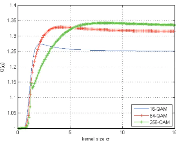
2.Q(σ)is calculated numerically for each modulation. Fig.3 shows the compensation
factorQ(σ)for 16-QAM, 64-QAM and 256-QAM modulations when using the MSQD-ℓ1 algorithm. For the MSQD-ℓ1 and MSQD-ℓ2, we implement the same steps as the algorithm summarized in [12], using the appropriate cost functions and Q functions.
B. Results
To compare blind equalization approaches proposed in this report, with others existing in the literature, we choosed the same channel as the one used in [12]:
h= [0.2258,0.5161,0.6452,−0.5161]T
. (58)
Performance of the proposed MSQD-ℓ2 and MSQD-ℓ1 methods are compared with those of the CMA and SQD. The latter was compared with the algorithms of CMA, Benveniste-Goursat (BG), Dual mode (DM)-CMA and its Stop-And-Go extension (SAG-DM-CMA). It was proved that the SQD method yields better performance. In the following, we show that the performance of MSQD-ℓ1 and MSQD-ℓ2 are better than those of SQD. Thus, the algorithms that we propose also perform better than the CMA, BG, DM-CMA and SAG-DM-CMA. For simulations, we employed an equalizer of length Lw = 21 initialized using
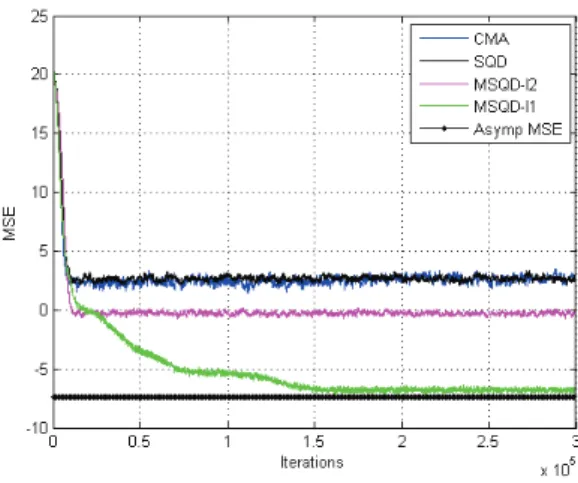
the tap-centered strategy. Table (I) below summarizes the parameters which were used to draw the curves in Fig.{4, 5, 6}. To compare the performance of the proposed algorithms in terms of convergence speed, we fixed the step sizeµsuch as they
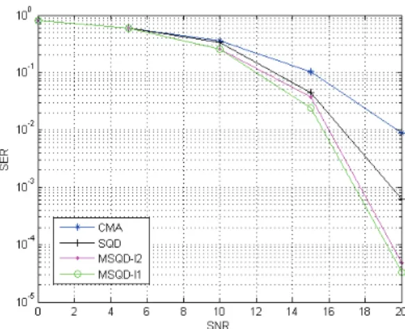
converge with the same speed. Thus, in Fig.4, Fig.5 and Fig.6, we can clearly notice that MSQD-ℓ2 and MSQD-ℓ1 outperform the SQD and CMA algorithms in terms of residual error for 16-QAM, 64-QAM and 256-QAM modulations. On the other hand, when we oblige the algorithms to converge to the same MSE in Fig.7 and Fig.8, we notice that MSQD-ℓ2 and MSQD-ℓ1 converge faster. All these figures validate the MSQD-ℓ1 performance analysis that we have conducted, since the experimental curve of the MSQD-ℓ1 converges to the theoretical one. To study the performance of the proposed algorithms as a function of the SNR, we draw in Fig.9 the Symbol Error Rate (SER) for the CMA, SQD, MSQD-ℓ2 and MSQD-ℓ1 algorithms between SNR = 0dB and SNR=20dB for a 16-QAM modulation. It is clear in this figure that the MSQD-ℓ1 algorithm outperforms the other algorithms in terms of the SER.
VII. CONCLUSION
In this report, we have proposed new criteria for kernel based blind equalization techniques that force the pdf of the real and imaginary parts of the equalizer output to match that of the true constellation real and imaginary parts by employing the Parzen window method to estimate the data pdf. Performance of the proposed methods has been compared with that of CMA and SQD. We have shown that they converge faster with a reduced residual error. The behaviour of the MSQD-ℓ1, most powerful proposed method, has been examined by relating the motion of the parameter estimate errors to a deterministic ODE. The analysis that we have conducted and simulation results prove that the MSQD-ℓ1 algorithm brings further validation of the pdf fitting approach for equalization in digital transmission.
TABLE I
PARAMETER VALUES USED FOR SIMULATIONS
16 QAM CMA SQD MSQD-l2 MSQD-l1 µ 3.5×10⁻⁵ 10−4 1.3 ×10⁻⁴ 7.7 ×10⁻⁴ a - 3.5 3.5 1.5 b - −9.5 −9.5 −1 1−α - 5×10⁻³ 5 ×10⁻³ 5 ×10⁻³ E0 - 7 7 5 64 QAM µ 3.3×10⁻⁷ 1.2 ×10⁻⁶ 9 ×10⁻⁷ 4.7 ×10⁻⁵ a - 3.5 3 2 b - −2 −18 −10 1−α - 10−3 10−2 10−3 E0 - 5 7 6.5 256 QAM µ 4×10⁻⁸ 1.5 ×10⁻⁷ 1.5 ×10⁻⁷ 7 ×10⁻⁵ a - 3.5 2.5 4 b - −4.5 −15 −1 1−α - 5×10⁻⁵ 10−4 2 ×10⁻⁴ E0 - 7 20 7
Fig. 3. Numerically obtained compensation factorQ(σ)in the case of MSQD-l1 algorithm.
Fig. 4. MSE (dB) for 16-QAM and SNR=30 dB.
Fig. 6. MSE (dB) for 256-QAM and SNR=30 dB.
Fig. 7. MSE (dB) for 16-QAM and SNR=30 dB.
Fig. 9. SER for CMA, SQD, MSQD-l2 and MSQD-l1 algorithms.
REFERENCES
[1] A. H. Sayed,Adaptive filters. John Wiley & Sons, Inc., Hoboken, New Jersey, 2008.
[2] Y. Sato, “A method of self-recovering equalization for multilevel amplitude-modulation systems,”IEEE Transactions on Communica-tions, vol. 23, no. 6, pp. 679 – 682, June 1975.
[3] D. Godard, “Self-recovering equalization and carrier tracking in two-dimensional data communication systems,”IEEE Transactions on Communications, vol. 28, no. 11, pp. 1867 – 1875, November 1980.
[4] J. Treichler and B. Agee, “A new approach to multipath correction of constant modulus signals,”IEEE Transactions on Acoustics, Speech and Signal Processing, vol. 31, no. 2, pp. 459 – 472, April 1983.
[5] K. N. Oh and Y. O. Chin, “Modified constant modulus algorithm: blind equalization and carrier phase recovery algorithm,” inIEEE International Conference on Communications, ICC Seattle, ’Gateway to Globalization’,, vol. 1, June 1995, pp. 498 –502.
[6] ——, “New blind equalization techniques based on constant modulus algorithm,” in Global Telecommunications Conference, GLOBECOM, IEEE, vol. 2, November 1995, pp. 865 –869.
[7] D. Jones, “A normalized constant-modulus algorithm,” inConference Record of the Twenty-Ninth Asilomar Conference on Signals, Systems and Computers, vol. 1, November 1995, pp. 694 –697.
[8] I. Santamaria, C. Pantaleon, L. Vielva, and J. Principe, “A fast algorithm for adaptive blind equalization using order-αrenyi’s entropy,”
ICASSP, 2002.
[9] J. Sala-Alvarez and G. Vazquez-Grau, “Statistical reference criteria for adaptive signal processing in digital communications,”IEEE Transactions on Signal Processing, vol. 45, no. 1, pp. 14 –31, january 1997.
[10] I. Santamaria, C. Pantaleon, L. Vielva, and J. Principe, “Adaptive blind equalization through quadratic pdf matching,”Proceedings of the European Signal Processing Conference, Toulouse, France, September 2002.
[11] M. Lazaro, I. Santamaria, C. Pantaleon, D. Erdogmus, K. E. Hild II, and J. C. Principe, “Blind equalization by sampled pdf fitting,”
[12] M. Lazaro, I. Santamaria, D. Erdogmus, K. Hild, C. Pantaleon, and J. Principe, “Stochastic blind equalization based on pdf fitting using parzen estimator,”IEEE Transactions on Signal Processing, vol. 53, no. 2, pp. 696 – 704, february 2005.
[13] A. Benveniste, M. Metivier, P. Priouret, and S. Wilson, Adaptive algorithms and stochastic approximations. Berlin ; New York : Springer, cop, 1990.
[14] D. W. Scott,Multivariate density estimation theory, practice, and visualization. John Wiley & Sons, Inc., New York, 1992. [15] E. Parzen, “On estimation of a probability density function and mode,”The Annals of Mathematical Statistics, September 1962. [16] I. Santamaria, C. Pantaleon, L. Vielva, and J. C. Principe, “A fast algorithm for adaptive blind equalization using order-α renyi’s
entropy,”ICASSP, 2002.
[17] J. Principe, D. Xu, Q. Zhao, J. Fisher III, and C. a. Pantaleon, “Learning from examples with information theoretic criteria,”Journal of VLSI signal processing, vol. 26, pp. 61 – 77, 2000.
[18] C. C. Cavalcante, F. Rodrigo, P. Cavalcanti, and J. C. M. Mota, “A pdf estimation-based blind criterion for adaptive equalizaion,”
International Telecommunications Symposium, 2002.
[19] J. Yang, J.-J. Werner, and G. Dumont, “The multimodulus blind equalization and its generalized algorithms,” IEEE Journal on Communications, vol. 20, no. 5, pp. 997 –1015, June 2002.
[20] C. Laot and N. Le Josse, “A closed-form solution for the finite length constant modulus receiver,” in International Symposium on Information Theory. ISIT, september 2005, pp. 865 –869.
[21] T. Chonavel,Statistical Signal Processing. Springer, 2003.
[22] L. Garth, “A dynamic convergence analysis of blind equalization algorithms,”IEEE Transactions on Communications, vol. 49, no. 4, pp. 624 –634, April 2001.
[23] Y. Li and K. Liu, “Static and dynamic convergence behavior of adaptive blind equalizers,”IEEE Transactions on Signal Processing, vol. 44, no. 11, pp. 2736 –2745, November 1996.
VIII. APPENDIX
A. Calculation of the maximum possible range for µ
Let us notey¯(n) =w∗x(n). At convergence,y(n)−y¯(n)is small and we can apply the taylor expansion to the function φ(y(n))(see Eq.(37)) aty¯(n). Then,
φ(yn) = φ(¯y(n)) +φ′(¯y(n))(y(n)−y¯(n))
= φ(¯y(n)) +φ′(¯y(n))(Hsf (n) +b(n))Tǫ(n) (59) where ǫ(n) =w(n)−w∗and Hsf (n) +b(n) =x(n).
In addition, we have
Thus, substractingw∗in both sides of Eq.(60) and using Eq.(59), we find that
ǫ(n+ 1) =ǫ(n)−µ φ(¯y(n))x(n)∗+φ′(¯y(n))(Hsf (n) +b(n))Tǫ(n)(Hf∗s∗(n) +b∗(n)) (61)
Taking the expectation on the both side of Eq.(61) and using the independence betweeny¯(n)andǫ(n), as it was assumed in [22], we get
E[ǫ(n+ 1)] = E[ǫ(n)]−µ E[φ(¯y(n))x∗(n)]
+ E[(Hf∗s∗(n) +b∗(n))φ′(ey(n))(Hsf (n) +b(n))T]E[ǫn] (62) In [23], the authors proved that E[φ(¯y(n))x∗(n)] = 0 when the cost function approaches one of its minima. Thus, Eq.(62) can be simplified to E[ǫ(n+ 1)] =ILw−µ(σ2sHf∗FeHfT+σb2E[φ′(¯yn)]ILw) E[ǫ(n)] (63) where Fe= σ12 sE s∗(n)φ′(¯y(n))s(n)T. Consequently E[ǫ(n+ 1)] =ILw−µ(σ2sHf∗FeHf T+ σb2E{φ′(ye(n))}ILw) n E[ǫ(0)] (64)
This yields the following condition upon the step size of the algorithm for convergence of the mean error :
0< µ < 2 λmax
(65)
where λmax is the largest eigenvalue of σs2Hf∗FeHfT +σb2E[φ′(¯y(n))]ILw.
B. Diagonalization ofRg in the basis U∗
Rg = −E H(w∗,x(n))H(w∗,x(n))H = −Eφ(s(nk))x∗(n)xT(n)φ(s(nk))∗ = −H∗E|φ(s(nk))|2s(n)sT(n)HT−E|φ(s(nk))|2b∗(n)bT(n) = −H∗DHT −σb2E |φ(s(nk))|2 (66)
where, D =diag(d1, ..., d1, d2, d1, ..., d1) withd1 =σ2sE
|φ(s(nk))|2 and d2 = E|s(nk)|2|φ(s(nk))|2 . We have cheked numerically that |d2−d1 d1 |
2 is very small (around 10−4). Then, we can consider that D ≃ d
following expression of Rg: Rg ≃ −d1H∗IL+Lw−1H T −σb2E |φ(s(nk))|2 ≃ −E|φ(s(nk))|2 σs2H∗H T+ σb2ILw ≃ −E|φ(s(nk))|2 U∗ΛxUT ≃ U∗ΛgUT (67) where Λg(i, i)≃ −E|φ(s(nk))|2λi.
Campus de Brest Technopôle Brest-Iroise CS 83818 29238 Brest Cedex 3 France +33 (0)2 29 00 11 11 www.telecom-bretagne.eu