Block Coordinate Descent for Sparse NMF

1

Block Coordinate Descent for Sparse NMF

Vamsi K. Potluru Department of Computer Science,

University of New Mexico ismav©cs.unm.edu Jonathan Le Roux Mitsubishi Electric Research Labs

leroux©merl.com

Vince D. Calhoun

Sergey M. Plis Mind Research Network,

splis©mrn.org

Barak A. Pearlmutter Department of Computer Science, National University of Ireland Maynooth

barak©cs.nuim.ie

Electrical and Computer Engineering, UNM and Mind Research Network

vcalhoun©mrn.org

Thomas P. Hayes Department of Computer Science,

University of New Mexico hayes©cs.unm.edu

Abstract

Nonnegative matrix factorization (NMF) has become a ubiquitous tool for data analysis. An important variant is the sparse NMF problem which arises when we explicitly require the learnt features to be sparse. A natural measure of sparsity is the La norm, however its optimization is NP-hard. Mixed norms, such as Ll/L2 measure, have been shown to model sparsity robustly, based on intuitive attributes that such measures need to satisfy. This is in contrast to computationally cheaper alternatives such as the plain L1 norm. However, present algorithms designed for optimizing the mixed norm L1

/L

2 are slow and other formulations for sparse NMF have been

pro-posed such as those based on L1 and La norms. Our proposed algorithm

allows us to solve the mixed norm sparsity constraints while not sacrificing computation time. We present experimental evidence on real-world datasets that shows our new algorithm performs an order of magnitude faster com-pared to the current state-of-the-art solvers optimizing the mixed norm and is suitable for large-scale datasets.

Introduction

Matrix factorization arises in a wide range of application domains and is useful for extracting the latent features in the dataset (Figure 1). In particular, we are interested in matrix factorizations which impose the following requirements:

• nonnegativity • low-rankedness • sparsity

Nonnegativity is a natural constraint when modeling data with physical constraints such as chemical concentrations in solutions, pixel intensities in images and radiation dosages for cancer treatment. Low-rankedness is useful for learning a lower dimensionality represen-tation. Sparsity is useful for modeling the conciseness of the representation or that of the

latent features. Imposing all these requirements on our matrix factorization leads to the sparse nonnegative matrix factorization (SNMF) problem.

SNMF enjoys quite a few formulations [2, 14, 13, 11, 24, 17, 25, 26] with successful applica-tions to single-channel speech separation [27] and micro-array data analysis [17, 25]. However, algorithms [14, 11] for solving SNMF which utilize the mixed norm of 11/12 as their sparsity measure are slow and do not scale well to large datasets. Thus, we develop an efficient algorithm to solve this problem and has the following ingredients:

• A theoretically efficient projection operator ( O(m log m)) to enforce the user-defined sparsity where m is the dimensionality of the feature vector as opposed to the previous approach [14].

• Novel sequential updates which provide the bulk of our speedup compared to the previously employed batch methods [14, 11].

input

data

PCA

fastiCA

sparse

PCA

dictionary

learning

k-means

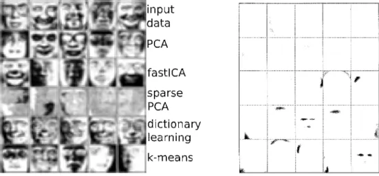
Figure 1: (Left) Features learned from the ORL dataset2_{with various matrix factorization} methods such as principal component analysis (PCA), independent component analysis (ICA), and dictionary learning. The relative merit of the various matrix factorizations depends on both the signal domain and the target application of interest. (Right) Features learned under the sparse NMF formulation where roughly half the features were constrained to lie in the interval [0.2, 0.4] and the rest are fixed to sparsity value 0.7. This illustrates the flexibility that the user has in fine tuning the feature sparsity based on prior domain knowledge. vVhite pixels in this figure correspond to the zeros in the features.

2

Preliminaries and Previous Work

In this section, we give an introduction to the nonnegative matrix factorization (NMF) and SNMF problems. Also, we discuss some widely used algorithms from the literature to solve them.

Both these problems share the following problem and solution structure. At a high-level, given a nonnegative matrix X of size m x n, we want to approximate it with a product of two nonnegative matrices W, H of sizes m x T and T x n, respectively:

(1) X:::::oWH.

The nonnegative constraint on matrix H makes the representation a conical combination of features given by the columns of matrix W. In particular, NMF can result in sparse representations, or a parts-based representation, unlike other factorization techniques such as principal component analysis (PCA) and vector quantization (VQ). A common theme in

2

the algorithms proposed for solving these problems is the use of alternating updates to the matrix factors, which is natural because the objective function to be minimized is convex in W and in H, separately, but not in both together. Much effort has been focused on optimizing the efficiency of the core step of updating one of W, H while the other stays fixed.

2.1 Nonnegative Matrix Factorization

Factoring a matrix, all of whose entries are nonnegative, as a product of two low-rank non-negative factors is a fundamental algorithmic challenge. This has arisen naturally in diverse areas such as image analysis

[20],

micro-array data analysis

[17],

document clustering

[31],

chemometrics

[19],

information retrieval

[12]

and biology applications [4]. For further appli-cations, see the references in the following papers

[1,

7].

We will consider the following version of the NMF problem, which measures the reconstruc-tion error using the Frobenius norm

[21]:

(2) w~u 211X- WHII} s.t. 1 w;::: 0, H;::: 0, 11Wjll2

=

1, Vj E {1, ... ,r}

where

2':

is element-wise. vVe use subscripts to denote column elements. Simple multiplica-tive updates were proposed by Lee and Seung to solve the NMF problem. This is attracmultiplica-tive for the following reasons:

• Unlike additive gradient descent methods, there is no arbitrary learning rate pa-rameter that needs to be set.

• The nonnegativity constraint is satisfied automatically, without any additional pro-jection step.

• The objective function converges to a limit point and the values are non-increasing across the updates, as shown by Lee and Seung

[21].

Algorithm 1 is an example of the kind of multiplicative update procedure used, for instance, by Lee and Seung

[21].

The algorithm alternates between updating the matrices Wand H (we have only shown the updates for H~those for Ware analogous).

Algorithm 1 nnls-mult(X, W, H) 1: repeat wTx 2: H

=

H0 WTWH" 3: until convergence 4: Output: Matrix H.

Here, 0 indicates wise (Hadamard) product and matrix division is also element-wise. To remove the scaling ambiguity, the norm of columns of matrix W are set to unity. Also, a small constant, say 10-9_{, is added to the denominator in the updates to avoid} division by zero.

Besides multiplicative updates, other algorithms have been proposed to solve the NMF problem based on projected gradient

[22],

block pivoting

[18],

sequential constrained opti-mization [6] and greedy coordinate-descent

[15].

2.2 Sparse Nonnegative Matrix Factorization

The nonnegative decomposition is in general not unique [9]. Furthermore, the features may not be parts-based if the data resides well inside the positive orthant. To address these issues, sparseness constraints have been imposed on the NMF problem.

Sparse NMF can be formulated in many different ways. From a user point of view, we can

split them into two classes of formulations: explicit and implicit. In explicit versions of SNMF [14, 11], one can set the sparsities of the matrix factors W, H directly. On the other

hand, in implicit versions of SNMF [17,

25],

the sparsity is controlled via a regularization parameter and is often hard to tune to specified sparsity values a priori. However, the algorithms for implicit versions tend to be faster compared to the explicit versions of SNMF. In this paper, we consider the explicit sparse NMF formulation proposed by Hoyer [14]. To make the presentation easier to follow, vve first consider the case where the sparsity is imposed on one of the matrix factors, namely the feature matrix W -the analysis for the symmetric case where the sparsity is instead set on the other matrix factor H is analogous. The case where sparsity requirements are imposed on both the matrix factors is dealt with in the Appendix. The sparse NMF problem formulated by Hoyer [14] with sparsity on matrix

W is as follows:

min f(W, H) =!IIX- WHII} s.t. W

2:

0, H

2:

0,

W,H 2

(3) IIWjlb = 1, sp(Wj)

=a,

'1/j E {1, · · · ,r}

Sparsity measure for a d-dimensional vector x is given by:

(4) sp(x) =

Vd-

llxlldllxll2

Vd-1

The sparsity measure ( 4) defined above has many appealing qualities. Some of which are as follows:

• The measure closely models the intuitive notion of sparsity as captured by the L0 norm. So, it easy for the user to specify sparsity constraints from prior knowledge of the application domain.

• Simultaneously, it is able to avoid the pitfalls associated with directly optimizing the Lo norm. Desirable properties for sparsity measures have been previously ex-plored [16] and it satisfies all of these properties for our problem formulation. The properties can be briefly summarized as: (a) Robin Hood- Spreading the energy from larger coordinates to smaller ones decreases sparsity, (b) Scaling - Sparsity is invariant to scaling, (c) Rising tide - Adding a constant to the coordinates decreases sparsity, (d) Cloning- Sparsity is invariant to cloning, (e) Bill Gates - One big coordinate can increase sparsity, (f) Babies - coordinates with zeros increase sparsity.

• The above sparsity measure enables one to limit the sparsity for each feature to lie in a given range by changing the equality constraints in the SNMF formulation (3)

to inequality constraints [11]. This could be useful in scenarios like fl'viRI brain

analysis, where one would like to model the prior knowledge such as sizes of artifacts are different from that of the brain signals. A sample illustration on a face dataset is shown in Figure 1 (Right). The features are now evenly split into two groups of local and global features by choosing two different intervals of sparsity.

A gradient descent-based algorithm called Nonnegative Matrix Factorization with Sparse-ness Constraints (NMFSC) to solve SNMF was proposed [14]. Multiplicative updates were used for optimizing the matrix factor which did not have sparsity constraints spec-ified. Heiler and Schni:irr[ll] proposed two new algorithms which also solved this prob-lem by sequential cone programming and utilized general purpose solvers like MOSEK (http: I /www. mosek. com). vVe will consider the faster one of these called tangent-plane constraint (TPC) algorithm. However, both these algorithms, namely NMFSC and TPC, solve for the whole matrix of coefficients at once. In contrast, we propose a block coordinate-descent strategy which considers a sequence of vector problems where each one can be solved in closed form efficiently.

3

The Sequential Sparse NMF Algorithm

We present our algorithm which we call Sequential Sparse

NMF (SSNMF)

to solve the SNMF problem as follows:

First, we consider a problem of special form which is the building block (Algorithm 2) of our SSNMF algorithm and give an efficient, as well as exact, algorithm to solve it. Second, we describe our sequential approach (Algorithm 3) to solve the subproblem of SNMF. This uses the routine we developed in the previous step. Finally, we combine our routines developed in the previous two steps along with standard solvers (for instance Algorithm 1) to complete the SSNMF Algorithm (Algorithm 4).

3.1 Sparse-opt

Sparse-opt routine solves the following subproblem which arises when solving problem (3):

(5) maxbT y s.t.

IIYII1

=

k,

IIYII2

=

1

y;::_o

where vector b is of size m. This problem has been previously considered [14], and an algorithm to solve it was proposed which we will henceforth refer to as the Projection-Royer. Similar projection problems have been recently considered in the literature and solved efficiently [ 10, 5].

Observation 1. For any i, j 1 we have that if b; :;:> bj 1 then y; :;:> Yj.

Let us first consider the case when the vector b is sorted. Then by the previous observation, we have a transition point p that separates the zeros of the solution vector from the rest. Observation 2. By applying the Cauchy-Schwarz inequality on y and the all ones vector, we get p :;:> k2

.

The Lagrangian of the problem (5) is :

Setting the partial derivatives of the Lagrangian to zero, we get by observation 1:

m m

LYi

=

k,

LYT

= 1

b;

+ p,(p)

+

A.(p)y;

=

0, ViE {1, 2, · · ·

,p}

r;=O,ViE {1,·0 0 ,p} Yi

=

O,Vi E {p+ 1, · · · ,m}

where we account for the dependence of the Lagrange parameters .\, p, on the transition point p. We compute the objective value of problem (5) for all transition points p in the range from k2 _{to m and select the one with the highest value. In the case, where} the vector b is not sorted, we just simply sort it and note down the sorting permutation vector. The complete algorithm is given in Algorithm 2. The dominant contribution to the running time of Algorithm 2 is the sorting of vector b and therefore can be implemented in 0( m log m) time3_{. Contrast this with the running time of Projection-Hoyer whose worst} case is O(m2) [14, 28].

3.2 Sequential Approach ~Block Coordinate Descent

Previous approaches for solving SNMF [14, 11] use batch methods to solve for sparsity constraints. That is, the whole matrix is updated at once and projected to satisfy the con-straints. We take a different approach of updating a. column vector at a. time. This gives us the benefit of being able to solve the subproblem (column) efficiently and exactly. Subse-quent updates can benefit from the newly updated columns resulting in faster convergence as seen in the experiments.

3_{This can be further reduced to linear time by noting that we do not need to fully sort the input} in order to find P*·

Algorithm 2 Sparse-opt(b,k)

1: Set a= sort(b) and p* = rn. Get a mapping 1r such that a; = b1r(i) and aj

2

aHl for all valid i, j.

2: Compute values of J.L(P), >..(p) as follows: 3: for p E

{lk

2

l,m}

_do 1--'---=->..(p)

= _

v2::f~,ar-(I:l'~,a,)2 (p-k2) 4: 5: 6: 7: 8: 9: J.L(p)

=

_Lf~,ai _i£)..(p) p p if

a(p)

<

-J.L(p) then p*

=

p -1 break end if 10: end for S t - ai+f.t(p') w· {1 *} d t th · 11: e x; - -· ,\(p*) , v~ E , · · · ,p an o zero o erw1se.

12: Output: Solution vector y where Yrr(i) = x;.

In particular, consider the optimization problem (3) for a column j of the matrix W while fixing the rest of the elements of matrices W, H:

- 1 2 T

min f(Wj) =

-2g[[Wj[[ 2

+u

Wj s.t. [[Wj[[2 = 1, [[Wj[[l = k Wj::>O

where g = HJ Hj and u = -XHJ + ~i#j W;(HHT)ij· This reduces to the problem (5) for which we have proposed an exact algorithm (Algorithm

2).

We update the columns of the matrix factor W sequentially as shown in Algorithm 3. vVe call it sequential for we update the columns one at a time. Note that this approach can be seen as an instance of block coordinate descent methods by mapping features to blocks and the Sparse-opt projection operator to a descent step.

Algorithm 3 sequential-pass(X, W, H)

1:

c

= -XHT + WHHT

2: G =HHT

3: repeat

4: for j = 1 tor (randomly) do

5:

uj

=

c j - w j c j j 6: t = Sparse-opt(-Uj,k). 7: C=C+(t-Wj)G} 8: Wj

=t.

9: end for 10: until convergence 11: Output: Matrix W.

3.3 SSNMF Algorithm for Sparse NMF

We are now in a position to present our complete Sequential Sparse NMF (SSNMF) algo-rithm. By combining Algorithms 1, 2 and 3, we obtain SSNMF (Algorithm 4).

Algorithm 4 ssnmf(X, W, H) 1: repeat 2: W = sequential-pass(X, W, H) 3: H

=

nnls-mult(X, W, H) 4: until convergence 5: Output: Matrices W, H.

4

Implementation Issues

For clarity of exposition, we presented the plain vanilla version of our SSNMF Algorithm 4. We now describe some of the actual implementation details.

• Initialization: Generate a positive random vector v of size m and obtain z

=

Sparse-opt(v,k) where k

=

.jiii-

cxvm

-1 (from equation (4)). Use the solu-tion z and its random permutations to initialize matrix W. Initialize the matrix H

to uniform random entries in [0, 1].

• Incorporating faster solvers: vVe use multiplicative updates for a fair comparison with NMFSC and TPC. However, we can use other NNLS solvers [22, 18, 6, 15] to solve for matrix H. Empirical results (not reported here) show that this further speeds up the SSNMF algorithm.

• Termination: In our experiments, we fix the number of alternate updates or equiv-alently the number of times we update matrix W. Other approaches include spec-ifying total running time, relative change in objective value between iterations or approximate satisfaction of KKT conditions.

• Sparsity constraints: We have primarly considered the sparse NMF model as for-mulated by Hoyer [14]. This has been generalized by Heiler and Schnorr [11] by relaxing the sparsity constraints to lie in user-defined intervals. Note that, we can handle this formulation

[11]

by making a trivial change to Algorithm

3.

5

Experiments and Discussion

In this section, we compare the performance of our algorithm with the state-of-the-art NMFSC and TPC algorithms [14, 11]. Running times for the algorithms are presented when applied to one synthetic and three real-world datasets. Experiments report reconstruction error

(II

X-

WHIIF)

instead of objective value for convenience of display. For all experiments on the datasets, we ensure that our final reconstruction error is always better than that of the other two algorithms. Our algorithm was implemented in MATLAB (http: I lwww. math works. com) similar to NMFSC and TPC. All of our experiments were run on a 3.2Ghz Intel machine with 24GB of RAM and the number of threads set to one.

5.1 Datasets

For comparing the performance of SSNMF with NMFSC and TPC, we consider the following synthetic and three real-world datasets :

• Synthetic: 200 images of size 9 x 9 as provided by Heiler and Schnorr [11] in their code implementation.

• CBCL face dataset consists of 2429 images of size 19 x 19 and can be obtained at http:llcbcl.mit.edulcbcllsoftware-datasetsiFaceData2.html.

• ORL: Face dataset that consists of 400 images of size 112 x 92 and can be ob-tained at http: I lwww. cl. cam. ac. uklresearchldtglattarchivelfacedatabase. html. http:llwww.kyb.tuebingen.mpg.delbethgelvanhaterenlimll. We use 400 of these images in our experiments.

• sMRI: Structural MRI scans of 269 subjects taken at the John Hopkins University were obtained. The scans were taken on a single 1.5T scanner with the imaging parameters set to 35mm TR, 5ms TE, matrix size of 256 x 256. We segment these images into gray matter, white matter and cerebral spinal finid images, using the software program SPM5 (http:/ /www.fil.ion.ucl.ac.uk/spm/softwarc/spm5/), followed by spatial smoothing with a Gaussian kernel of 10 x 10 x 10 mm. This results in images which are of size 105 x 127 x 46

~0.4 c 0 u (lJ Ul -;;;- 0.2 E F

1-•-

Projection Hoyer Sparse Opt

0.2

o.ou.~~-L----~u.~~-L----~~~~~---LJ~~~~---~

0 2 4 0 2 40 2 40 2 4

Problem size (omitted scale factor= 100,000)

Figure 2: Mean running times for Sparse-opt and the Projection-Royer are presented for random problems. The x-axis plots the dimension of the problem while they-axis has the running time in seconds. Each of the subfigures corresponds to a single sparsity value in {0.2, 0.4, 0.6, 0.8}. Each datapoint corresponds to the mean running time averaged over 40 runs for random problems of the same fixed dimension.

10'1 10° 101 10'2 time (seconds) 10'1 10° 101 10'2 time (seconds) 10'1 10° 101 10'2 time (seconds) 10'1 10° 101 time (seconds)

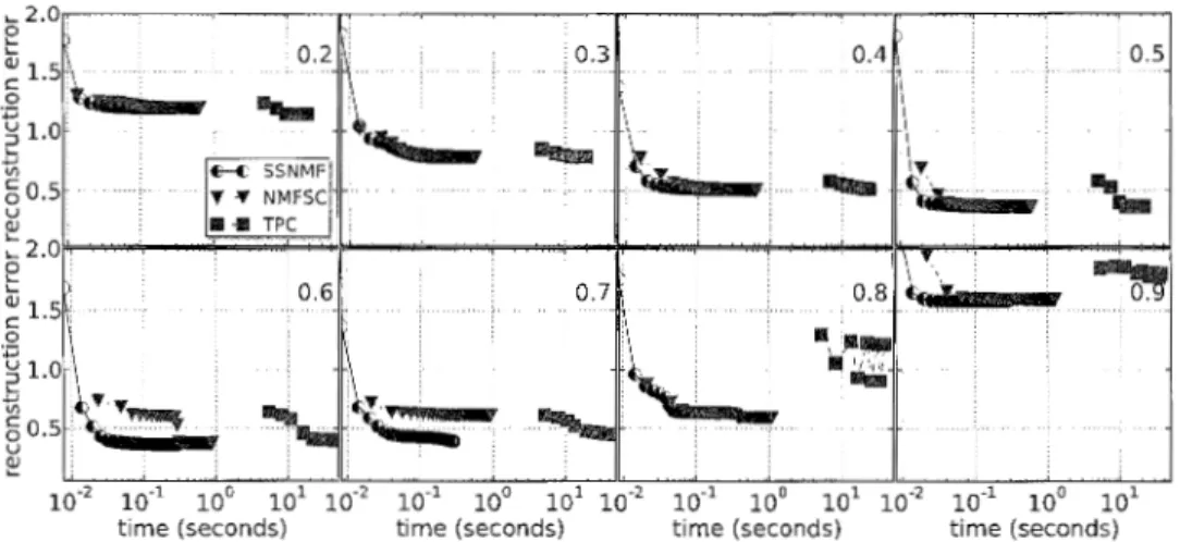
Figure 3: Running times for SSNMF and NMFSC and TPC algorithms on the synthetic dataset where the sparsity values range from 0.2 to 0.8 and number of features is 5. Note that SSNMF and NMFSC are over an order of magnitude faster than TPC.

5.2 Comparing Performances of Core Updates

We compare our Sparse-opt (Algorithm 2) routine with the competing Projection-Royer [14]. In particular, we generate 40 random problems for each sparsity constraint in {0.2, 0.4, 0.6, 0.8} and a fixed problem size. The problems are of size 2i x 100 where i takes integer values from 0 to 12. Input coefficients are generated by drawing samples uniformly at random from [0, 1]. The mean values of the running times for Sparse-opt and the Projection-Royer for each dimension and corresponding sparsity value are plotted in Figure 2.

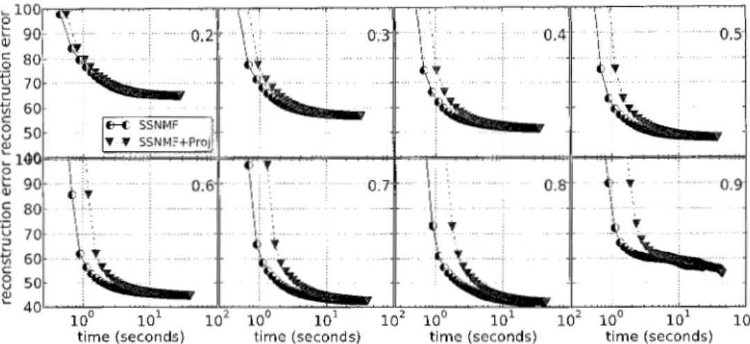
We compare SSNMF with SSNMF+Proj on the CBCL dataset. The algorithms were run with rank set to 49. The running times are shown in Figure 6. 'vVe see that in low-dimensional datasets, the difference in running times are very small.

5.3 Comparing Overall Performances

SSNMF versus NMFSC and TPC: We plot the performance of SSNMF against NMFSC and TPC on the synthetic dataset provided by Heiler and Schnorr [11] in Fig-ure 3. 'vVe used the default settings for both NMFSC and TPC using the software provided

Figure 4: Convergence plots for the ORL dataset with sparsity from [0.1, 0.8] for the NMFSC and SSNMF algorithms. Note that we are an order of magnitude faster, especially when the sparsity is higher.

... 0.1 _{0.2 0.3 0.4}

v.

103 104 103 104 103 104 103 104

time (seconds) time (seconds) time (seconds) time (seconds)

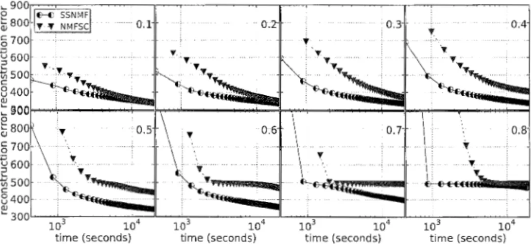
Figure 5: Running times for SSNMF and NMFSC algorithms for the sMRI dataset with rank set to 40 and sparsity values of a from 0.1 to 0.8. Note that for higher sparsity values we converged to a lower reconstruction error and are also noticeably faster than the NMFSC algorithm.

by the authors. Our experience with TPC was not encouraging on bigger datasets and hence we show its performance only on the synthetic dataset. It is possible that the performance of TPC can be improved by changing the default settings but we found it non-trivial to do so.

SSNMF versus NMFSC: To ensure fairness, we removed logging information from NMFSC code [14] and only computed the objective for equivalent number of matrix updates as SSNMF. We do not plot the objective values at the first iteration for convenience of display. However, they are the same for both algorithms because of the shared initialization . We ran the SSNJ\IIF and NMFSC on the ORL face dataset. The rank was fixed at 25 in both the algorithms. Also, the plots of running times versus objective values are shown in Figure 4 corresponding to sparsity values ranging from 0.1 to 0.7. Additionally, we ran our SSNMF algorithm and NMFSC algorithm on a large-scale dataset consisting of the structurallVIRI images by setting the rank to 40. The running times are shown in Figure 5.

~ 100 2 90 0.5 \.... Qi c ₈₀ 0 .

..,

u ₇₀ 2 ..., 60 Vl c 0 ₅₀ u

~

1\bO 2 90 0.9 \.... _0.8 (])

Figure 6: Running times for SSNMF and SSNMF+Proj algorithms for the CBCL face dataset with rank set to 49 and sparsity values ranging from 0.2 to 0.9

5.4 Main Results

We compared the running times of our Sparse-opt routine versus the Projection-Royer and found that on the synthetically generated datasets we are faster on average.

Our results on switching the Sparse-opt routine with the Projection-Royer did not slow down our SSNMF solver significantly for the datasets we considered. So, we conclude that the speedup is mainly due to the sequential nature of the updates (Algorithm 3).

Also, vve converge faster than NMFSC for fewer number of matrix updates. This can be seen by noting that the plotted points in Figures 4 and 5 are such that the number of matrix updates are the same for both SSNMF and NMFSC. For some datasets, we noted a speedup of an order of magnitude making our approach attractive for computation purposes. Finally, we note that we recover a parts-based representation as shown by Hoyer

[14].

An example of the obtained features by NMFSC and ours is shown in Figure 7.

(a) sparsity 0.5 (b) sparsity 0.6 (c) sparsity 0. 75

Figure 7: Feature sets from NMFSC algorithm (Left) and SSNMF algorithm (Right) using the ORL face dataset for each sparsity value of a in {0.5,0.6,0.75}. Note that SSNMF algorithm gives a parts-based representation similar to the one recovered by NMFSC.

6

Connections to Related Work

Other S.:\MF formulations have been considered by Hoyer [13], Morup ct al. [24] , Kim and Park [17], Pascual-Montano et al. [25] (nsNMF) and Peharz and Pernkopf [26]. SNMF formulations using similar sparsity measures as used in this paper have been considered for applications in speech and audio recordings [30, 29].

vVe note that our sparsity measure has all the desirable properties, extensively discussed by Hurley and Rickard [16], except for one ( "doning"). Cloning property is satisfied when

two

vectors

of same sparsity when concatenated maintain their sparsity value. Dimensions in our optimization problem are fixed and thus violating the cloning property is not an issue. Compare this with the L1 norm that satisfies only one of these properties (namely "rising tide"). Rising tide is the property where adding a constant to the elements of a vector decreases the sparsity of the vector. Nevertheless, the measure used in Kim and Park is based on the L1 norm. The properties satisfied by the measure in Pascual-Montano et al. are unclear because of the implicit nature of the sparsity formulation.

Pascual-Montano et al. [25] claim that the SNMF formulation of Hoyer, as given by prob-lem (3) does not capture the variance in the data. However, some transformation of the sparsity values is required to properly compare the two formulations [14, 25]. Preliminary results show that the formulation given by Hoyer [14] is able to capture the variance in the data if the sparsity parameters are set appropriately. Peharz and Pernkopf [26] propose to tackle the La norm constrained NMF directly by projecting from intermediate uncon-strained solutions to the required La constraint. This leads to the well-known problem of getting stuck in local minima. Indeed, the authors re-initialize their feature matrix with an NNLS solver to recover from the local suboptimum. Our formulation avoids the local minima associated with La norm by using a smooth surrogate.

7

Conclusions

vVe have proposed a new efficient algorithm to solve the sparse NMF problem. Experiments demonstrate the effectiveness of our approach on real datasets of practical interest. Our algorithm is faster over a range of sparsity values and generally performs better when the sparsity is higher. The speed up is mainly because of the sequential nature of the updates in contrast to the previously employed batch updates of Hoyer. Also, we presented an exact and efficient algorithm to solve the problem of maximizing a linear objective with a sparsity constraint, which is an improvement over the heuristic approach in Hoyer.

Our approach can be extended to other NMF variants [13]. Another possible application is the sparse version of nonnegative tensor factorization. A different research direction would be to scale our algorithm to handle large datasets by chunking [23] and/ or take advantage of distributed/parallel computational settings [3].

Acknowledgement

The first author would like to acknowledge the support from NIBIB grants 1 R01 EB 000840 and 1 ROl EB 005846. The second author was supported by NIMH grant 1 R01 MH076282-0l. The latter two grants were funded as part of the NSF /NIH Collaborative Research in Computational Neuroscience Program.

References

[1] Sanjeev Arora, Rong Ge, Ravindran Karman, and Ankur Moitra. Computing a nonneg-ative matrix factorization- provably. In Proceedings of the 44th symposium on Theory of Computing, STOC '12, pages 145-162, New York, NY, USA, 2012. ACM.

[2] Michael W Berry, Murray Browne, Amy N Langville, V Paul Pauca, and Robert J

Plemmons. Algorithms and applications for approximate nonnegative matrix factor-ization. Computational Statistics 8 Data Analysis, 52(1):155-173, 2007.

[3] Joseph K. Bradley, Aapo Kyrola, Danny Bickson, and Carlos Guestrin. Parallel coor-dinate descent for Ll-regularized loss minimization. In ICML, pages 321-328, 2011. [4] G. Buchsbaum and 0. Bloch. Color categories revealed by non-negative matrix

factor-ization of munsell color spectra. Vision resear-ch, 42(5):559-563, 2002. [5] Yunmei Chen and Xiaojing Ye.

arXiv:1101.6081, 2011.

[6] A. Cichocki and A. H. Pharr. Fast local algorithms for large scale nonnegative matrix and tensor factorizations. IEICE Transactions on Fundamentals of Electronics, 92: 708-721, 2009.

[7]

J. E. Cohen and U. G. Rothblum. Nonnegative ranks, decompositions, and factor-izations of nonnegative matrices. LineaT Algebra and its Applications, 190:149-168, 1993.

[8] Chris Ding, Tao Li, ~Wei Peng, and Haesun Park. Orthogonal nonnegative matrix t-factorizations for clustering. In PToceedings of the 12th ACM SIGKDD international

confeTence on Knowledge discoveTy and data mining, KDD '06, pages 126-135, New York, NY, USA, 2006. ACM.

[9] David Donoho and Victoria Stodden. When does non-negative matrix factorization give a correct decomposition into parts? In Sebastian Thrun, Lawrence Saul, and Bernhard Scholkopf, editors, Advances in Neural InfoTmation Processing Systems 16. MIT Press, Cambridge, MA, 2004.

[10] .John Duchi, Shai Shalev-Shwart7,, Yoram Singer, and Tushar Chandra. Efficient pro-jections onto the 11-ball for learning in high dimensions. In PToceedings of the 25th international confeTence on Machine learning, pages 272-279, 2008.

[11] Matthias Heiler and Christoph Schnorr. Learning sparse representations by non-negative matrix factorization and sequential cone programming. The Journal of

Ma-chine Leaming ReseaTch, 7:2006, 2006.

[12] T. Hofmann. Unsupervised learning by probabilistic latent semantic analysis. Machine Leaming, 42(1):177-196, 2001.

[13] P. 0. Hoyer. Non-negative sparse coding. In Neural NetwoTks for Signal PTOcessing, 2002. Pmceedings of the 2002 12th IEEE Wor·kshop on, pages 557-565, 2002.

[14] Patrik 0. Hoyer. Non-negative matrix factorization with sparseness constraints. J.

Mach. Learn. Res., 5:1457-1469, December 2004.

[15] C. J. Hsieh and I. Dhillon. Fast coordinate descent methods with variable selection for non-negative matrix factorization. ACM SIGKDD InteTnation ConfeTence on Knowl-edge Discovery and Data Mining, page xx, 2011.

[16] Niall Hurley and Scott Rickard. Comparing measures of sparsity. IEEE Trans. Inf. TheoT., 55:4723-4741, October 2009.

[17] Hyunsoo Kim and Haesun Park. Sparse non-negative matrix factorizations via alter-nating non-negativity-constrained least squares for microarray data analysis. BioinfoT-matics, 23(12) :1495-1502, 2007.

[18] Jingu Kim and Haesun Park. Toward faster nonnegative matrix factorization: A new algorithm and comparisons. Data Mining, IEEE International Conference on, 0:353-362, 2008.

[19] W. H. Lawton and E. A. Sylvestre. Self modeling curve resolution. Technometrics, pages 617-633, 1971.

[20] D. D. Lee and H. S. Seung. Learning the parts of objects by non-negative matrix factorization. Nature, 401(6755):788-791, October 1999.

[21] Daniel D. Lee and Sebastian H. Seung. Algorithms for non-negative matrix factoriza-tion. In NIPS, pages 556-562, 2000.

[22] Chih-Jen Lin. Projected gradient methods for nonnegative matrix factorization. Neural Camp., 19(10):2756-2779, October 2007.

[23] Julien Mairal, Francis Bach, Jean Ponce, and Guillermo Sapiro. Online learning for matrix factorization and sparse coding. The Joumal of Machine Leaming ReseaTch, 11:19-60, 2010.

[24]

Morten M0rup, Kristofi'er Hougaard Madsen, and Lars Kai Hansen. Approximate LO constrained non-negative matrix and tensor factorization. In

ISCAS,

pages 1328-1331, 2008.

[25] A. Pascual-Montano, J. M. Carazo, K. Kochi, D. Lehmann, and R. D. Pascual-Marqui. Nonsmooth nonnegative matrix factorization (nsNMF). Pattern Analysis and I'Vfachine Intelligence, IEEE Transactions on, 28(3):403-415, March 2006.

[26] R. Peharz and F. Pernkopf. Sparse nonnegative matrix factorization with 1°-constraints. Neurocomputing, 2011.

[27] M. N. Schmidt and R. K. Olsson. Single-channel speech separation using sparse non-negative matrix factorization. In Intenwt·ional Conference on Spoken Language

Pro-cessing (INTERSPEECH), volume 2, page 1. Citeseer, 2006.

[28] Fabian J Theis, Kurt Stadlthanner, and Toshihisa Tanaka. First results on uniqueness of sparse non-negative matrix factorization. In Proceedings of the 13th European Signal Processing Conference (EUSIPC005), 2005.

[29] Thomas Virtanen. Monaural sound source separation by nonnegative matrix factor-ization with temporal continuity and sparseness criteria. Audio, Speech, and Language Processing, IEEE Transactions on, 15(3):1066-1074, 2007.

[30] Felix Weninger, Jordi Feliu, and Bjorn Schuller. Supervised and semi-supervised sup-pression of background music in monaural speech recordings. In Acoustics, Speech and Signal Processing (ICASSP), 2012 IEEE International Conference on, pages 61--64. IEEE, 2012.

[31] W. Xu, X. Liu, and Y. Gong. Document clustering based on non-negative matrix factorization. In Proceedings of the 26th annual international ACM SIGIR conference

on Researd! and development in informaion retr·ieval, pages 267-273. ACM, 2003.

Appendix

Bi-Sparse NMF

In some applications, it is desirable to set the sparsity on both matrix factors. However, this can lead to the situation where the variance in the data is poorly captured [25]. To ameliorate this condition, we formulate it as the following optimization problem and call it as Bi-Sparse NMF: (6) . 1 mm -IIX-WDHII} W,H,D2 s.t.W 2 O,H 2 O,D 2 0 IIWjll2

=

1,sp(Wj)

=

a,\:lj E {1,··· ,r} IIHill2

=

1, sp(Hi)

=

(3, '1/i E {1, · · · , r}

where D is a r x r matrix. In the above formulation, we constrain the L2 norms of the

columns of matrix W to unity. Similarly, we constrain the L2 norms of rows of matrix H

to be unity. This scaling is absorbed by the matrix D. Note that this formulation with the matrix D constrained to be diagonal is equivalent to the one proposed in Hoyer when both the matrix factors have their sparsity specified.

Vve can solve for the matrix D with any NNLS solver. A concrete algorithm is the one presented in Ding et al. and is reproduced here for convenience (Algorithm 5). If D is a diagonal matrix, we only update the diagonal terms and maintain the rest at zero. Algo-rithms 1 and 5 can be sped up by pre-computing the matrix products which are unchanged during the iterations.

Also, the matrix D captures the variance of the dataset when we have sparsity set on both the matrices W, H.

Algorithm 5 Diag-mult(X, W, H,

D)

repeat

D

=

D _{C WTWDHH}WTXH 1

until convergence