Hourly diffuse solar radiation in the presence of
clouds and other environmental parameters:
the city of São Paulo.
Claudia Furlan
Department of Statistical Sciences University of Padua
Italy
Amauri Pereira de Oliveira
Group of Micrometeorology, Department of Atmospheric Sciences Institute of Astronomy, Geophysics and Atmospheric Sciences University of São Paulo
Brazil
Abstract: The network of stations for diffuse solar radiation measurements is scarce through the world, while global solar radiations are available for many locations. Since 1960s numerous studies have been developed to model diffuse fraction on the clearness index (that is based on global radiation). Recent comparative studies, based on polynomial regression, corroborated that hourly values of diffuse solar radiation are not very well modeled by only clearness index, even though there is a strong relation.
On the other hand, neural network techniques were used to model satisfactorily the hourly values of diffuse radiation combining the clearness index with some environmental parameters such as latitude, longitude, time of the day, month, rainfall, air temperature, relative humidity and atmospheric pressure. Even tough neural network techniques gives satisfactory results, they are not a user-friendly tool for non-experts.
In this work we propose a multiple linear regression that takes into account the clearness index, the particulate matter (PM10), the cloud effect and some
environmental parameters available in conventional meteorological stations. The model we propose is easier to understand than the neural network and performs better.
Keywords: diffuse solar radiation, clearness index, clouds, pollution, regression
Contents
1. Introduction ... 1
2. Climate of São Paulo and data description ... 2
3. Model description ... 5
4. Results... 7
5. Validation of the model ... 9
6. Conclusion ... 13
Hourly diffuse solar radiation in the presence of clouds and other
environmental parameters: the city of São Paulo.
Claudia Furlan
Department of Statistical Sciences University of Padua
Italy
Amauri Pereira de Oliveira
Group of Micrometeorology, Department of Atmospheric Sciences Institute of Astronomy, Geophysics and Atmospheric Sciences University of São Paulo
Brazil
Abstract: The network of stations for diffuse solar radiation measurements is scarce through the world, while global solar radiations are available for many locations. Since 1960s numerous studies have been developed to model diffuse fraction on the clearness index (that is based on global radiation). Recent comparative studies, based on polynomial regression, corroborated that hourly values of diffuse solar radiation are not very well modeled by only clearness index, even though there is a strong relation.
On the other hand, neural network techniques were used to model satisfactorily the hourly values of diffuse radiation combining the clearness index with some environmental parameters such as latitude, longitude, time of the day, month, rainfall, air temperature, relative humidity and atmospheric pressure. Even tough neural network techniques gives satisfactory results, they are not a user-friendly tool for non-experts.
In this work we propose a multiple linear regression that takes into account the clearness index, the particulate matter (PM10), the cloud effect and some environmental parameters available in conventional meteorological stations. The
model we propose is easier to understand than the neural network and performs better.
Keywords: diffuse solar radiation, clearness index, clouds, pollution, regression
1. Introduction
Few energy production technologies have a little impact on the environment as solar energy technologies. The solar energy source is free and abundant and the energy generated by light does not produce any air pollution or hazardous waste. The most widespread solar energy technologies, which are currently in use, are the solar photovoltaic and the solar thermal energy. The use of free energy of the sun would allow freeing us from dependence of unreliable sources of oil and would reduce the impact of power outages. Actually, solar energy is not economically competitive with conventional alternatives if we consider capital costs, operating and maintenance costs and financial costs. However, considering the actual situation about the greenhouse effects and the oil depletion perspective, many countries passed laws that provide financial incentives to encourage an early adoption of solar energy technologies. However, with regard to PV for example, the next for the solar electricity is to be competitive without these incentives, reducing costs and making these systems more efficient, affordable and available.
Estimate solar radiation field at the surface is rather difficult and it can not be done numerically without simplifying the role of cloud, moisture and other minor atmospheric gases and aerosol casting doubts about the degree of realism. More realistic simulations require information about cloud and atmospheric gases and particles that are not available. Diffuse solar radiation is an important component of the surface radiation budget. It is difficult to measure. Diffuse solar radiation depends on surface albedo and the composition of atmosphere, mainly clouds and particulate matter. Since 1960s, with the pioneer work of Liu and Jordan (1960), numerous studies have been developed to model diffuse fraction (ratio of diffuse solar radiation at the surface to global at the surface) on clearness index (ratio of global solar radiation at the surface to solar radiation at the top of the atmosphere). A comparative study, based on polynomial regression, has
been proposed by Jacovides et al. (2006) and it corroborated, with the previous findings, that hourly values of diffuse fraction are not very well modeled by only clearness index, even though there is a strong relation. One of the models compared by Jacovides et al. (2006) is a 4th degree polynomial
proposed by Oliveira et al. (2002), in which the diffuse fraction was modeled using only the clearness index (nevertheless, for smallest and largest values of the clearness index, the model is constant). The model performed well for monthly and daily values but was not able to differentiate cloud effects on the diffuse solar radiation for hourly values. In facts, clouds seriously affect the proportion of diffuse radiation on the total radiation, especially “in tropical regions, like Brazil, where cloud activity is a dominant feature of local climate” (Soares, 2004). To overcome these difficulties Soares et al. (2004) applied neural network technique to estimate hourly values of diffuse solar radiation. In this case cloud and other effects were taken into consideration implicitly by the pattern recognition ability of neural network technique. The only difficult on this particular technique was that neural network is rather cumbersome to use by others than the ones that developed the algorithm. The set of coefficients derived in the neural network technique can not be made available as in the case of regression models.
In this work we propose a multiple linear regression that takes into account the clearness index, the particulate matter (PM10), the cloud effect explicitly and some environmental parameters available
in conventional meteorological stations.
2. Climate of São Paulo and data description
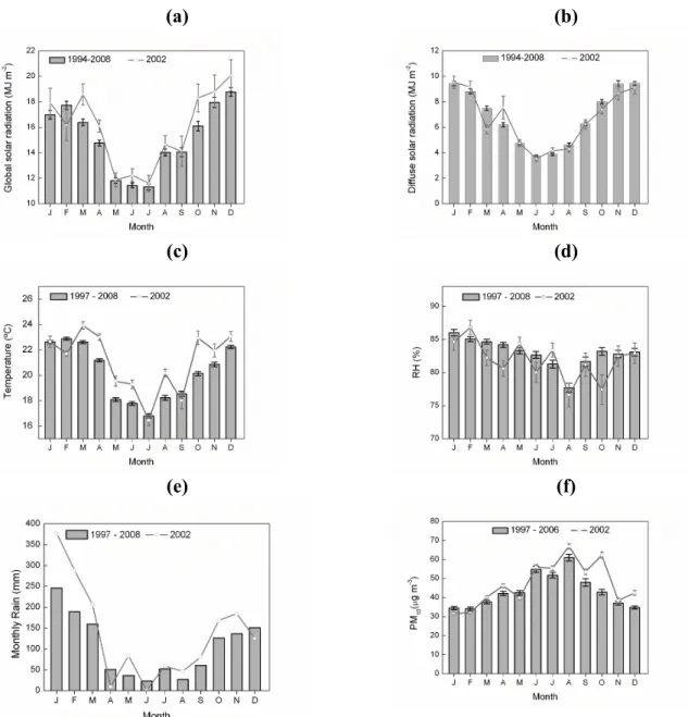
The City of São Paulo is located in the State of São Paulo (Fig. 1a), Brazil, at approximately 770 m above MSL and 60 km westward from the Atlantic Ocean (Fig. 1b). The city of São Paulo, with about 11 millions habitants, together with 39 other smaller cities, forms the Metropolitan Region of São Paulo. This region, located about 60 km far from the Atlantic Ocean, is occupied by 20.5 millions of habitants and by more of 7 millions of vehicles distributed over an area of 8,051 km2. It is the largest urban area in South America and one of the 10 largest in the world (Oliveira et al., 2002; Codato et al., 2008). Its climate - typical of subtropical regions of Brazil - is characterized by a dry winter during June-August and a wet summer during December-March. The minimum values of daily monthly-averaged temperature and relative humidity occur in July and August (16o C and
74 %, respectively), and the minimum monthly-accumulated precipitation occurs in August (35 mm). The maximum value of daily monthly-averaged temperature occurs in February (22.5o C) and the maximum value of daily monthly-averaged relative humidity occurs from December through January and from March through April (80%).
Global and diffuse solar radiation, temperature, relative humidity, pressure and precipitation measurements were taken on a micrometeorological platform located at the building top of the Institute of Astronomy, Geophysics and Atmospheric Sciences of the University of São Paulo, at the University Campus, in the western side of the city of São Paulo (Fig. 1c), at 744 m above MSL (23033'35''S; 46043'55”W). All measurements are taken with a sampling frequency of 0.2 Hz and stored as 5-minutes averages. All observations used in this work it was carried out during 2002 in the city of São Paulo, Brazil (23º33’34’’S, 46º44’01’’W). Fig. 2 compares the monthly average values of global, diffuse, temperature, relative humidity, precipitation measured during 2002 and from 1997 to 2008. There one see that most of the meteorological parameters and PM10 in 2002 are
very close the long term statistics, indicating that 2002 can be considered representative of the dominate climate conditions in São Paulo.
A pyranometer, model 8-48, built also by Eppley Lab. Inc, measured global solar irradiance. This sensor has been periodically calibrated using as secondary standard a spectral precision pyranometer model PSP, from Eppley Lab. Inc. The calibration consists of running, at least once a year, side-by-side, both pyranometers continuously during 2 to 7 days (Oliveira et al., 2002). The
(a)
(b)
(c)
Figure 1. Geographic position of the (a) State of São Paulo, (b) City of São Paulo and (c) IAG, PEFI and C. Cesar.
solar irradiance at the top of the atmosphere (extraterrestrial) was estimated analytically (Iqbal, 1983) considering the solar constant equal to 1366 W m-2 (Frölich and Lean, 1998).
The air temperature and relative humidity were estimated using a pair of thermistor and capacitive sensors from Vaisala. According to the manufacturer the air temperature and relative humidity are
measured with an accuracy of 0.1 oC and 2 % respectively, for a range of temperature 0 and 40 oC and 10 to 90 %. Pressure was measured using a capacitive transducers manufactured by Setra Inc. In this study it was included also hourly values of particulate matter (PM10) measured at the surface
in the Cerqueira Cesar station (Fig. 1c) belonging to the air quality monitoring network of São Paulo State Environmental Protection Agency in 2002 (CETESB, 2006).
The fraction of sky cover and type of cloud are estimated every hour from 0700 LT to 2400 LT in the meteorological station located in the South of São Paulo City indicated by PEFI (Fig. 1c). The type of cloud information includes traditional low, middle and high level clouds. It was included in this analysis cloud type, fraction of the sky covered by cloud in oktas and the cloud type estimated hourly at the meteorological surface station locate in the “Parque Estadual Fontes do Ipiranga” (PEFI, Fig. 1c).
(a) (b)
(c) (d)
(e) (f)
Figure 2. Annual evolution of (a) global solar radiation (b) diffuse solar radiation, (c) temperature, (d) relative humidity, (e) rain and (f) particulate matter observed in the city of São Paulo.
3. Model description
The model is based on the existing relationship between Kd and Kt. and how it changes in terms of
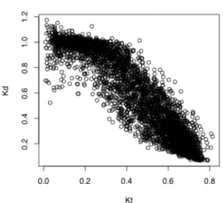
air temperature, relative humidity, atmospheric pressure, concentration of particulate matter, cloud cover and cloud type, time of the day, month of the year. Figure 3 indicates the relation between diffuse fraction and clearness index that will be explored in this work to develop the regression model. The model was developed considering 75% of observations. The remaining 25% was used for validation.
The best compromise between empirical evidence and knowledge is achieved by the following segmented regression between Kd and Kt:
(1)
This expression represents a straight line that changes slope in Kt = c, without discontinuities. For
Kt < c the line is characterized by intercept and slope , while for Kt > c by intercept
and slope . The estimate of change point c is 0.228 (st. err. 0.006), of is 0.97 (st. err. 0.01), of is -0.07 (st. err. 0.08) and of is -1.64 (st. err. 0.08). The hypothesis of a constant relationship between Kt and Kd before Kt = 0.2276 (that is ) was tested through a T-test.
The hypothesis was not rejected with a P-value of 0.23. Model (1) is then reduced to
(2)
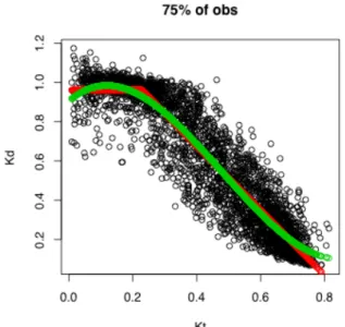
where has been replaced by . The estimate of is 0.961 (st. err. 0.003) and of is -1.65 (st. err. 0.01). The red line in Figure 4 shows model (2), while the green line shows the third degree polynomial function proposed by Jacovides et al. (2006), that Jacovides himselself assented as the best performing model in his comparative study. The two models are essentially different for values of Kt before the change point: while model (2) is constant, the third degree polynomial function is
first increasing and then decreasing. We think that since model (2) is more coherent with the knowledge existing between Kd and Kt, the polynomial trend before the change point that Jacovides
found should be attributed to a variability of data that could be modelled taking into account, for example, other source of information.
Subsequently, we modelled Kd on the variables presented in Section 2, through a multiple
regression where the relationship between Kd and Kt is as in (2)
(3)
where c has been estimated in (1) as 0.228, is an indicator function that assumes value 1 if (Kt>c) and 0 otherwise, and (X2,…, Xp) are the other environmental variables collected in this
study.
The continuous quantitative variables are:
• Temperature (oC): the minimum observed value is 8.721, the maximum is 34.79; • Pressure (mb): the minimum observed value is 910, the maximum is 949.6; • PM10 (µg m-3): the minimum observed value is 0.45, the maximum is 281.10.
Figure 3. Diffuse radiation fraction (Kd) versus Clearness Index (Kt). The number of observations
is 3887.
These variables have been initially categorized into 7 categories through the 2.5th, 5th, 25th, 75th, 95th, 97.5th quantiles, but the final number of categories for each variable has been detected by using the Nested Model Test. It allows to merge together those categories that do not show any significant differences.
The discrete quantitative variables (that will be categorized by using the Nested Model Test) are
• Cloudiness Index (fraction of the sky covered by clouds): the minimum value is 0 (that
corresponds to 0%) and the maximum 10 (that corresponds to 100%);
• Hour of the day (LT): the minimum value is 6.5 and the maximum is 18.5 (that is 6.5 p.m.);
With regard to the time evolution we considered the categorical variable “Month”.
The cloud effect topic has been faced by defining the following dichotomous variables (that expresses presence or absence):
• Low altitude clouds:
o Stratocumulus;
• Mixed altitude clouds:
o Cumulunimbus;
• Middle altitude clouds:
o Altocumulus
o Altostratus
• High altitude clouds:
o Cirrocumulus
o Cumulus
• Clear sky (in the three levels)
• Clear sky in the low level (and covered sky in the upper levels) • Cloudy in the low level (and clear sky in the upper levels) • Cloudy in the middle level (and clear sky in the other two levels) • Cloudy in the high level (and clear sky in the other two levels)
In particular, the specification of the last four variables addresses the question of identify the effect of low, middle, high clouds separately.
Figure 4. Diffuse radiation fraction (Kd) versus Clearness Index (Kt). The green line represents a
third degree polynomial function (Jacovides et al., 2006), while the red line represents the segmented regression, as indicated in (2). These functions have been estimated on the 75% of observations (n=2915).
4. Results
Table 1 shows the results of regression model (3) with only the variables and the interactions come out to be significant.
The estimate of the coefficient of Kt is -1.293: that is, for fixed values of all the other explanatory
variables, every increase of 1 in the value of Kt, the value of Kd decreases of 1.293.
All the other coefficients of Table 1 refer to categorical or dichotomous variables and to understand the meaning of coefficients it is necessary to detect a reference category. For dichotomous variables we decided to use as reference category the absence of the event described, and for categorical variables the lowest category. In this way, for each variable, coefficients represent the average variation of Kd for the corresponding category, with respect to the reference category.
Four categories have been identified for Relative Humidity (see Table 1): the reference category is represented by values smaller than 61% (25th quantile). Coefficients are positive and increase with the increasing of relative humidity, detecting a positive relationship between relative humidity and
Kd. In particular, Kd increases of 0.032 in average if relative humidity is between 61% and 89%, if
compared with the reference category (RH<61%). Kd increases of 0.037 when relative humidity is
between 89% and 98%, while increases of 0.091 when relative humidity is bigger than 98%, if compared with the reference category.
Temperature has only two categories: the reference category is for values smaller than 15 oC (5th quantile) or bigger than 26 oC (75th quantile). The coefficient 0.013 means that Kd increases in
average of 0.013 when temperature is between 15 and 26 oC: this category may represent the typical temperature of a summer day without clouds.
Pressure has four categories and the reference category is for values smaller than 918 mb. As for relative humidity, coefficients are positive and increasing: for increasing values of pressure, Kd
increases.
Particulate matter has only two categories (reference category for values smaller than 25 µg m-3), but no differences were found to be significant between the two categories. Anyhow, it will be significant in association with a specific cloud pattern.
The reference category for Cloudiness Index is the fraction of covered sky between 0% and 20%. Coefficients of the other categories are positive and increasing. We highlight that Kd increases of
0.065 when CI=80% (with respect to the reference category), but it increases approximately of the double (with respect to the reference category) when CI=90% or CI=100% (0.122 and 0.148 respectively).
The reference value for hours of the day is represented by the early morning and the late afternoon hour (6.5, 7.5, 18.5 LT). Kd is bigger in the late morning and in the first afternoon (0.073 and 0.067
respectively). The reference category for the month is represented basically by the summer (December and January). With respect to summer, Kd decreases 0.016 in February, September,
October and November, 0.061 in March and April (autumn) and 0.068 in May, June, July and August (winter).
Taking into account the type of cloud, stratocumulus, altocumulus, altostratus, cirrocumulus and cumulus have a positive effect on Kd, since the coefficients are positive. Comparing the value of the
coefficients, we conclude that cumulus (high level) has a bigger impact. Since the coefficients of cumulonimbus and cirrus are -0.074 and -0.022 respectively, we can say that these two types of cloud have a negative effect on Kd. Looking at the negative coefficient of the clear sky (-0.028) we
can conclude that the effect of cirrus is similar of the effect of the clear sky, but the effect of cumulonimbus is approximately 3 times bigger than the effect of cirrus and clear sky (since cumulonimbus is often associated to strong precipitations, this should be due to the effect of washing the air from particles). The presence of the clear sky only in the low level has a negative effect (-0.046) that is double if compared with the effect of the presence of clear sky in all the three levels. Unexpectedly clouds in the low, middle and high level were not significant, probably because the impact of the type of cloud was stronger.
The coefficient of the interaction between clear sky (only low level) and PM10 (>25 µg m-3) is
0.051: it means that, even though the clear sky has a negative effect on Kd, when it is associated to
values of PM10 bigger than 25 µg m-3, Kd increases of 0.051.
The next group of interactions are among clouds at a middle level and high values of the cloudiness index. The coefficients are positive, meaning that the co-presence of middle clouds and high values of CI intensifies Kd. However, since coefficients decrease for increasing values of CI we can
conclude that, in presence of clouds at middle level, Kd is more exacerbated when the sky is 70%
-80% covered rather than is 100% covered.
The last four groups of interactions are among relative humidity and, respectively, clear sky, clouds at high level, middle level and low level. With respect to clear sky we obtained negative coefficients
that decrease when RH increases: even though RH increases Kd and clear sky decreases Kd, the co-
presence of clear sky and humidity has a negative impact on Kd. In particular, the negative impact is
bigger for high values of RH. On the contrary, the interaction between clouds in the low level and high values of relative humidity is positive: in other words, even though the relative humidity has already a positive impact on Kd, the presence of clouds in the low level and high values of relative
humidity makes Kd increasing again. Looking at the interactions among relative humidity and
clouds at high and middle levels, we can find a similarity with the pattern showed by the same interaction with clear sky. In this way, we can conclude that high and middle clouds, when interacting with humidity, behave more similarly to the clear sky than to clouds at low level.
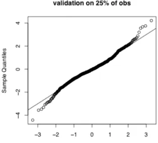
Figure 5. Validation of the model on the remaining 25% of observations. Q-Q Plot for the standardized residuals.
5. Validation of the model
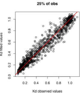
The model we proposed in Table 1 has been validated on the remaining 25% of observations. Figure 5 shows the Q-Q plot of the standardized residuals, that compares theoretical quantiles of a Normal distribution with the sample quantiles of the standardized residuals. The fit to the bisector is good except in the left and in the right end for a total 5.5% of points. Figure 6 shows observed valued of Kd against fitted values (25% of observations): the alignment to the bisector is
satisfactory. Figure 7 shows observed values of Kd (black points) and fitted valued of Kd (red stars)
with respect to Kt.
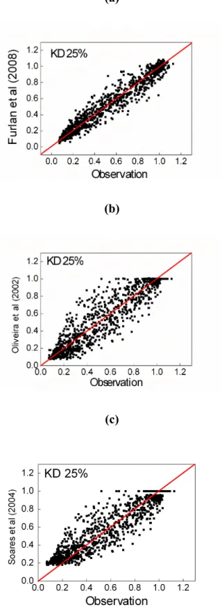
Figure 8 represents the comparison of the fitting performances among the model here proposed – panel (a) – the polynomial model proposed by Oliveira et al. (2002) – panel (b) – and the model built through the neural network by Soares et al. (2004) – panel (c). The performance of this model is much superior, both for the variability of points to the bisector and for the power of predictability for the farthest points. Since in meteorological literature it is common to model the diffuse fraction Kd to, then, evaluate the diffuse solar radiation (as Kd times the global solar radiation), in Figure 9
we show the behaviour of the 3 models from this points of view. The model proposed in this paper – panel (a) – performs much better if compared with the model of Oliveira et al. (2002) – panel (b)
– and of Soares et al. (2004) – panel (c), for a general reduction of variability and because it does not overestimate the diffuse solar radiation for values smaller than about 0.3-0.5, as in the other 2 models, and because it underestimates the diffuse solar radiation only for values larger than about 1.6 (that is, for clear sky).
Figure 6. Validation of the model on the remaining 25% of observations: observed vs fitted values. The red line is the bisector.
(a)
(b)
(c)
Figure 8: Fitted vs observed values for the model here proposed (a), for the polynomial model proposed by Oliveira et al. (2002) (b), and for the neural network model of Soares et al. (2004).
(a)
(b)
(c)
Figure 9: Estimates of the diffuse solar radiation (evaluated as fitted values of Kd times the
global solar radiation) for the model here proposed (a), for the polynomial model proposed by Oliveira et al. (2002) (b), and for the neural network model of Soares et al. (2004.)
6. Conclusion
This work, in its genuine simplicity, is innovative in the field of meteorology and it is principally an explorative study that can open several research issues. It allows to estimate the changepoint in the relation between the diffuse solar radiation and the clearness index, while in the previous works concerning polynomial models it was decided subjectively. Numerical variables as relative humidity, temperature, pressure, particular matter, fraction of the sky covered by clouds and hour of the day has been categorized in a few different levels that affect the diffuse radiation differently. Moreover, this model takes into account the most important environmental variables as previously it was faced only by the neural network techniques, with a simple statistical tool that is easy understandable by non-expert and that outlines clear relationships between the diffuse radiation and the explanatory variables. Indeed, it allowed to isolate and identify the effect of the environmental variables, as never been done before, especially for the cloud effects.
One limit of this study is the lack of information about precipitation. The diffuse fraction is much more variable when the sky is nearly total covered. Indeed, if the sky is covered but it does not rain the diffuse fraction increases, while if it rains the diffuse fraction decreases since the rain cleans the air from the particles.
A further development of this work could be re-organizing all the information in the dataset allowing a reduction of the number of variables. Moreover, we could try to restore the information of the precipitation through other variables in the dataset and, in this way, we could take into account the variability of the diffuse fraction due to the presence or the absence of precipitation with covered sky.
7. References
CETESB (2006) Technical report on air quality in the State of São Paulo – Environmental State Secretary, ISSN 0103–4103, São Paulo, Brazil, 137pp.
Codato G., Oliveira A.P., Soares J, Escobedo J.F., Gomes, E.N., and Pai A.D. (2008) Global and diffuse solar irradiances in urban and rural areas in southeast of Brazil, Theoretical and Applied Climatology, 93, 57-73.
Frölich C., Lean J. (1998) The sun’s total irradiance: cycles and trends in the past two decades and associated climate change uncertainties, Geophys Res Lett, 25, 4377–4380.
Iqbal M. (1983) An introduction to solar irradiance. Academic Press, New York, 390 pp.
Jacovides C.P., Tymvios F.S., Assimakopoulos V.D. (2006) Comparative study of various correlations in estimating hourly diffuse fraction of global solar diffusion, Renewable Energy,
31, 2492-2504.
Liu B.Y.H., Jordan R.C. (1960) The interrelationship and characteristic distribution of direct, diffuse and total solar radiation, Sol Energy, 4, 1-19.
Oliveira A.P., Escobedo J.F., Machado A.J., Soares J. (2002) Correlation models of diffuse solar radiation applied to the city of São Paulo, Brazil, Applied Energy, 71, 59-73.
Scarpa B., Azzalini A. (2004) Analisi dei dati e data mining, Springer.
Soares J., Oliveira A.P., Zlata Boznar M., Mlakar P., Escobedo J.F., Machado A.J. (2004) Modeling hourly diffuse solar-radiation in the city of São Paulo using a neural-network technique, Applied Energy, 79, 201-214.
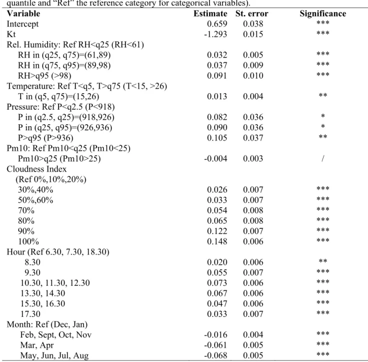
Table 1. Estimates and standard errors of the coefficients of variables in model (3). *significant at 5% level, ** significant at 1% level, *** significant at 0.1% level (label “qx” represents the x th-quantile and “Ref” the reference category for categorical variables).
Variable Estimate St. error Significance
Intercept 0.659 0.038 ***
Kt -1.293 0.015 ***
Rel. Humidity: Ref RH<q25 (RH<61)
RH in (q25, q75)=(61,89) 0.032 0.005 *** RH in (q75, q95)=(89,98) 0.037 0.009 *** RH>q95 (>98) 0.091 0.010 *** Temperature: Ref T<q5, T>q75 (T<15, >26) T in (q5, q75)=(15,26) 0.013 0.004 ** Pressure: Ref P<q2.5 (P<918) P in (q2.5, q25)=(918,926) 0.082 0.036 * P in (q25, q95)=(926,936) 0.090 0.036 * P>q95 (P>936) 0.105 0.037 ** Pm10: Ref Pm10<q25 (Pm10<25) Pm10>q25 (Pm10>25) -0.004 0.003 / Cloudness Index (Ref 0%,10%,20%) 30%,40% 0.026 0.007 *** 50%,60% 0.033 0.007 *** 70% 0.054 0.008 *** 80% 0.065 0.008 *** 90% 0.122 0.007 *** 100% 0.148 0.006 *** Hour (Ref 6.30, 7.30, 18.30) 8.30 0.020 0.006 ** 9.30 0.055 0.007 *** 10.30, 11.30, 12.30 0.073 0.006 *** 13.30, 14.30 0.067 0.006 *** 15.30, 16.30 0.047 0.006 *** 17.30 0.033 0.007 ***
Month: Ref (Dec, Jan)
Feb, Sept, Oct, Nov -0.016 0.004 ***
Mar, Apr -0.061 0.005 ***
Table 1 (Continuation) Stratocumulus (Low) 0.018 0.004 *** Cumulunimbus (Mixed) -0.074 0.013 *** Altocumulus (Middle) 0.015 0.006 * Altostratus (Middle) 0.019 0.006 ** Cirrus (High) -0.022 0.007 ** Cirrocumulus (High) 0.015 0.007 * Cumulus (High) 0.186 0.081 * Clear sky -0.028 0.012 *
Clouds – low level -0.011 0.007 /
Clouds – middle level -0.037 0.019 /
Clouds – high level -0.014 0.009 /
Clear sky – low level -0.046 0.018 *
Interactions
Clear sky low level – with
Pm10 (>q25) 0.051 0.018 **
Clouds middle level – with
Cloudness index=70% 0.201 0.083 *
Cloudness index=80% 0.109 0.031 ***
Cloudness index=90% 0.074 0.029 *
Cloudness index=100% 0.069 0.021 **
Clear sky – with
Rel. Humidity in (q25, q75) -0.037 0.010 ***
Rel. Humidity in (q75, q95) -0.070 0.018 ***
Rel. Humidity >q95 -0.089 0.029 **
Clouds high level – with
Rel. Humidity in (q25, q75) -0.047 0.011 ***
Rel. Humidity >q95 -0.077 0.032 *
Clouds middle level – with
Rel. Humidity in (q75, q95) -0.043 0.019 *
Rel. Humidity >q95 -0.063 0.024 **
Clouds low level – with
Working Paper Series
Department of Statistical Sciences, University of Padua
You may order copies of the working papers from by emailing to [email protected] Most of the working papers can also be found at the following url: http://wp.stat.unipd.it