ADVANCES IN INDEPENDENT COMPONENT ANALYSIS WITH APPLICATIONS TO DATA MINING

(1)

Helsinki University of Technology

Dissertations in Computer and Information Science

Espoo 2003 Report D4

ADVANCES IN INDEPENDENT COMPONENT ANALYSIS

WITH APPLICATIONS TO DATA MINING

Ella Bingham

Dissertation for the degree of Doctor of Science in Technology to be presented with due permission of the Department of Computer Science and Engineering for public examination and debate in Auditorium T2 at Helsinki University of Technology (Espoo, Finland) on the 12th of December, 2003, at 12 o’clock noon.

Helsinki University of Technology

Department of Computer Science and Engineering Laboratory of Computer and Information Science P.O.Box 5400

FIN-02015 HUT FINLAND

(2)

Laboratory of Computer and Information Science P.O.Box 5400 FIN-02015 HUT FINLAND Tel. +358-9-451 3272 Fax +358-9-451 3277 http://www.cis.hut.fi

Available in pdf format at http://lib.hut.fi/Diss/2003/isbn9512268205/

c

Ella Bingham

ISBN 951-22-6819-1 (printed version) ISBN 951-22-6820-5 (electronic version) ISSN 1459-7020

Otamedia Oy Espoo 2003

(3)

Bingham, E. (2003): Advances in independent component analysis with applica-tions to data mining. Doctoral thesis, Helsinki University of Technology, Dissertaapplica-tions in Computer and Information Science, Report D4, Espoo, Finland.

Keywords: independent component analysis, latent variable models, dimensionality reduc-tion, data mining, complex valued signals, random projecreduc-tion, regression, topic identificareduc-tion, 0-1 data.

ABSTRACT

This thesis considers the problem of finding latent structure in high dimensional data. It is assumed that the observed data are generated by unknown latent variables and their interactions. The task is to find these latent variables and the way they interact, given the observed data only. It is assumed that the latent variables do not depend on each other but act independently.

A popular method for solving the above problem is independent component analysis (ICA). It is a statistical method for expressing a set of multidimensional observations as a combination of unknown latent variables that are statistically independent of each other. Starting from ICA, several methods of estimating the latent structure in different problem settings are derived and presented in this thesis. An ICA algorithm for analyzing complex valued signals is given; a way of using ICA in the context of regression is discussed; and an ICA-type algorithm is used for analyzing the topics in dynamically changing text data. In addition to ICA-type methods, two algorithms are given for estimating the latent structure in binary valued data. Experimental results are given on all of the presented methods.

Another, partially overlapping problem considered in this thesis is dimensionality reduction. Empirical validation is given on a computationally simple method called random projection: it does not introduce severe distortions in the data. It is also proposed that random projection could be used as a preprocessing method prior to ICA, and experimental results are shown to support this claim.

This thesis also contains several literature surveys on various aspects of finding the latent structure in high dimensional data.

(4)

Preface

This work has been carried out at the Laboratory of Computer and Information Science (CIS) at Helsinki University of Technology during the years 1999–2003. The work has been funded by Helsinki Graduate School in Computer Science and Engineering (HeCSE) and the CIS laboratory. In addition, I have received grants from Ella and Georg Ehrnrooth Foundation, Finnish Cultural Foundation, Foundation of Technology, KAUTE Foundation and Nokia Foundation, all of which I am grateful for.

Professor Erkki Oja, the supervisor of my thesis, has been a fatherly and trustworthy figure for me. Docent Aapo Hyvärinen, the first of my two instructors, has introduced me to the fascinating world of ICA and scientific research in general. Professor Heikki Mannila, my second instructor, has fed my appetite with new problem domains, and has been of great support whenever needed. I feel obliged to all of these three gentlemen.

It has been a great honor for me to have two such distinguished pre-examiners: Professor Thomas Hofmann and Professor Helena Ahonen-Myka, whom I wish to express my gratitude. In addition, it will surely be a pleasant experience to defend my thesis against Dr Mark Plumbley, whom I thank for agreeing to act as my opponent.

I am severely indebted to my scientific collaborators. Especially I would like to thank Dr Ata Kabán for patiently introducing me to the secrets of probabilistic modeling, besides being a great friend. All of my co-authors — Docent Aapo Hyvärinen, Professor Heikki Mannila, Dr Ata Kabán, Professor Mark Girolami and Mr Jouni Seppänen — are experts in their fields, which has made my collaboration with each of them a true pleasure.

I could not imagine a better place to conduct research than the CIS laboratory. We have been blessed with excellent leaders: Professor Erkki Oja and Professor Olli Simula, who trust us enough to let us work freely, and who do their best to ensure us excellent material facilities. The atmosphere in the laboratory is active, yet pleasant and youthful. For this I wish to thank the whole of the personnel, especially Anne, Heli, Johan and Karthikesh. My parents have supported me in many ways during the writing of this thesis, which I truly appreciate. My dear husband Kenrick, the foremost source of happiness in my life, has been of great help. Thank you so much.

Espoo, November 24, 2003

(5)

v

Notation and abbreviations

a scalar constant

c scalar constant

d dimensionality ofxbefore dimensionality reduction f scalar-valued function of a scalar variable

g scalar-valued function of a scalar variable i index ofxi

j index ofsj orwj

k dimensionality ofxafter random projection m dimensionality ofxafter dimensionality reduction n number of latent components; dimensionality ofsory

p probability density function s independent latent component t observation index, time index x component of observed vectorx

y latent component ε scalar constant

π probability of a component θ parameter; set of parameters E expectation operator

N number of observed vectorsx

P probability

f vector-valued function of a vector variable

g vector-valued function of a vector variable

p column vector of probabilities

s column vector of independent latent components

w column vector of a projection direction

x observed column vector

y column vector of latent components

xT vectorxtransposed (applicable to any vector)

(8)

A mixing matrix; topic matrix

B binary noise matrix

D matrix of eigenvalues

E matrix of eigenvectors

P matrix of probabilities

R random projection matrix

S matrix of independent latent componentss

V random matrix in random sampling and quantization

W unmixing matrix

X matrix of observed vectorsx Y matrix of latent components BSS blind signal separation EM expectation-maximization GTM generative topographic mapping ICA independent component analysis IR information retrieval

LDA latent Dirichlet allocation LSA latent semantic analysis MAP maximum a posteriori ML maximum likelihood MLP multilayer perceptron

MPCA multinomial principal component analysis MSE mean squared error

NMF nonnegative matrix factorization PCA principal component analysis

PLSA probabilistic latent semantic analysis RP random projection

SNLP statistical natural language processing SOM self-organizing map

SSE sum of squared errors SVD singular value decomposition

(9)

1

Chapter 1

About the thesis

1.1 Scope of the thesis

This doctoral thesis considers the problem of finding latent structure in high dimensional data. Here the term latent means hidden, unknown or unobserved; the term structure refers to some regularities in the data;high dimensionalmay be tens or tens of thousands of dimensions, depending on the situation; anddatais any information that can be transformed into numerical values, most often represented as a matrix of multidimensional observations where each dimension corresponds to a variable whose value we can somehow measure. The aims in this thesis are to answer the question “What is there in the data?”, to form a simple representation of a large data set that is difficult to analyze as such, and to present the data in a form that is understandable to a human observer.

Throughout the thesis, it will be assumed that the observed data are generated by interactions between latent variables. The objective is to find out what these latent variables are and how they interact — this is the key to understanding what the data are about. The latent variables will be calledcomponents,sources ortopics: the data are composed of these latent variables, or the latent variables are the sources of variability in the data, or in particular in text document data the latent variables are the topics of discussion. Depending on the point of view, the “structure” in the data we referred to in the beginning is either due to the values taken by the latent variables or due to the way the latent variables interact. Throughout this thesis, we will assume that there are no inherent dependencies between the latent variables. In addition to revealing the latent structure in high dimensional data, another aim of this thesis is to present ways of reducing the dimensionality of the data. This aim overlaps partially with the first one: we wish to transform the data into a denser representation and only retain the most important aspects of the data.

Let us present an example of the problem of finding latent structure in the data. A popular example is the so called cocktail party problem: Imagine a room full of people discussing with each other. A few microphones, located at different positions in the room, collect the

(10)

sounds of mixed human voices and possible external noises. An outsider listening to the mixtures of sounds recorded by the microphone cannot decipher what was actually discussed in the room. The task now is to decompose the mixtures of sounds back into their original form, that is, human voices and external noises. These original sounds are called the latent sources, as they are “hidden” from the outsider listener. The task is often referred to as source separation. The computational methods discussed later in this thesis are aimed at solving problems similar to this one.

Although the above example is old and frequently cited, it is repeated here because it suits nicely some of the specific contributions of this thesis. Firstly, the sounds arriving at the microphones are more or less delayed and may contain echoes from nearby walls. This poses additional problems in decomposing the mixtures of sounds. One way to overcome these problems will be discussed in Chapter 3 of the thesis. Secondly, imagine that instead of people speaking, we observe their written conversations. A chat room in the Internet is like a big cocktail party where lots of people discuss different topics simultaneously. Again, an outsider cannot at first sight understand what people are discussing, as different discussions get intertwined as they appear on the computer screen. This problem is tackled in Chapters 5 and 6 of the thesis where we present methods for finding out the latent topics of a discussion. In short, the methods discussed in this thesis estimate the structure in the data by finding latent components whose interactions might have generated the data. We do not know which these latent components might be, neither do we know about the exact way they interact. Nevertheless, we are willing to assume that there are indeed some interactions, so that a typical observation is not generated by one latent component only. To cast more light on this, it may be helpful to contrast our approach with two well-known and different ones. First, the methods used to analyze the data in this thesis are unsupervised in contrast to supervised; that is, there is no teacher telling us whether our decomposition is correct or not. No labeled examples, with known input values and corresponding output values1

or with a known input-output structure, are given for building a model of the data. Instead, the unsupervised methods try to infer the structure of the data simply by looking at the values taken by the observed variables. Often it is even the case that no “correct” solution or structure exists and we can only try to give a “good enough” characterization of the data. Then the essential question is, how to characterize the goodness in a strict mathematical sense.

Second, a popular way of presenting the structure in high dimensional data is clustering: either the observed data points or the observed variables are organized into groups. We will not study the basic problem of clustering in this thesis. In a clustering problem, it is assumed that each observation (similarly, each observed variable) belongs to exactly one cluster. In contrast, we wish to allow the generation of an observation by several latent variables si-multaneously; using the terminology of clustering, we allow an observation (similarly, an observed variable) to belong to several clusters simultaneously. Also, in a basic clustering setting, the focus is either on clustering the observations or the observed variables. In our setting, the latent structure of the data gives rise to both the observations and the observed variables, and in a way we are clustering both of them simultaneously.

1

To be exact, labeled examples of predictor and predicted variables are used in the regression problem discussed in Chapter 4, as those are an essential element of regression estimation. Nevertheless, the structure in the data is unknown in this case, too.

(11)

1.2. Contributions of the thesis 3

In this thesis, the main method for analyzing latent structure in the data is independent component analysis(ICA), described in Chapter 2. ICA can also be seen as a way of dimen-sionality reduction, although that is not its primary aim. Several other methods for these two overlapping tasks will be discussed, too.

The original methods and intuitions behind ICA will be extended in various directions: into different kinds of data (complex valued in contrast to real valued, and binary valued in contrast to continuous valued) and into different problem settings (regression problems and information retrieval).

In this thesis, the point of view taken is often that ofdata mining. Data mining is a name used for a variety of computational methods and techniques for analyzing large data sets. The aim in data mining is to describe the data either in a global or a local level. Global descriptions include clustering, joint probability density estimation, or visualization of the data; local descriptions might be repeating or exceptional patterns in the data, or statistical dependencies between the variables. Although data mining is closely related to traditional statistical data analysis, it has a couple of distinguishing characteristics: the data are not originally aimed for a particular study and so the analyst cannot affect the process of data collection; the data set is often so large that its storage and retrieval must be carefully designed; the emphasis is on local aspects in addition to global behavior in the data. An introduction to data mining is given in [56] and data mining and statistics are compared in [46].

This thesis consists of an introductory part and six publications, listed in Section 1.3. Throughout the introductory part of the thesis, the reader is referred to the publications. They contain most of the contributions of this work and are self-explanatory. The deriva-tions, results and discussions of the publications are seldom repeated in this introductory part. It is assumed that the reader is familiar with the basics of linear algebra, probability and statistics.

1.2 Contributions of the thesis

The scientific contributions of this thesis include the following.

• Experimental results are given on using random projection as a method of dimensional-ity reduction. In particular, experimental results on the use of a sparse random matrix have not been presented elsewhere.

• The use of random projection as a data preprocessing method for independent compo-nent analysis (ICA) is suggested. Empirical validation is presented in the cases of ICA of image data, complex valued signals and text document data.

• A fast fixed-point ICA algorithm for separating linearly mixed complex valued source signals is presented and the local consistency of the estimator given by the algorithm is proved.

• Empirical validation of using ICA as a preprocessing method in nonlinear regression is given.

(12)

• It is shown that an ICA-type algorithm can successfully extract the topics of discussion in dynamically evolving natural language text.

• Two algorithms for the estimation of latent structure in binary valued data are given, together with empirical results.

• Literature surveys are given on each topic addressed in the thesis: latent variable decompositions, separation of complex valued signals, ICA-type methods in regression and in the analysis of text documents, and latent variable models of binary valued data.

1.3 Publications of the thesis

Publication 1. Ella Bingham and Aapo Hyvärinen. A fast fixed-point algorithm for independent component analysis of complex valued signals. International Journal of Neural Systems, 10(1):1–8, February 2000.

Publication 2. Ella Bingham and Heikki Mannila. Random projection in dimensional-ity reduction: applications to image and text data. In Foster Provost and Ramakrishnan Srikant, editors,Proceedings of the 7th ACM SIGKDD International Conference on Knowl-edge Discovery and Data Mining, pages 245–250, San Francisco, CA, USA, August 2001. Publication 3. Aapo Hyvärinen and Ella Bingham. Connection between multilayer per-ceptrons and regression using independent component analysis. Neurocomputing, 50(C):211– 222, January 2003.

Publication 4. Ella Bingham, Ata Kabán, and Mark Girolami. Topic identification in dynamical text by complexity pursuit. Neural Processing Letters, 17(1):69–83, 2003. Publication 5. Ella Bingham, Heikki Mannila, and Jouni K. Seppänen. Topics in 0-1 data. In David Hand, Daniel Keim, and Raymond Ng, editors, Proceedings of the 8th ACM SIGKDD International Conference on Knowledge Discovery and Data Mining, pages 450–455, Edmonton, Alberta, Canada, July 2002.

Publication 6. Jouni K. Seppänen, Ella Bingham, and Heikki Mannila. A simple al-gorithm for topic identification in 0-1 data. In Nada Lavrač, Dragan Gamberger, Ljupčo Todorovski, and Hendrik Blockeel, editors,Knowledge Discovery in Databases: PKDD 2003. 7th European Conference on Principles and Practice of Knowledge Discovery in Databases. Cavtat-Dubrovnik, Croatia, September 2003, Proceedings, number 2838 in Lecture Notes in Artificial Intelligence, pages 423–434. Springer, 2003.

Contents of the publications and the contributions of Ella Bingham

In Publication 1, an ICA algorithm for separating linear mixtures of complex valued source signals is presented. The fixed-point algorithm is somewhat similar to the FastICA algo-rithm [76, 70] which had been developed for real valued signals. The local consistency of the estimator given by the algorithm is proved, too. Ella Bingham was responsible for deriving the fixed-point algorithm, proving the theorem of the local consistency, planning and

(13)

con-1.4. Structure of the thesis 5

ducting the experiments reported in the paper, studying the relation to subspace methods, and mainly writing the manuscript.

In Publication 2, the use of random projection as a tool of dimensionality reduction is discussed. Extensive experiments on text document data and both noisy and noiseless images are presented. Also, experimental results on using a sparsely populated random matrix as presented by Achlioptas [1] are given — to the knowledge of the authors of the paper and Achlioptas, these are the first experiments on using sparse random projection. Ella Bingham planned and carried out all the experiments in the paper and wrote most of the manuscript. Publication 3 discusses the use of independent component analysis in regression. When only a subset of the variables are observed, ICA can be used to predict the values of missing vari-ables. It is shown that this kind of regression is closely related to regression by a multilayer perceptron (MLP) network. Ella Bingham was responsible for the experimental results in the paper.

In Publication 4, an ICA-type algorithm is applied to estimating the dynamically changing topics of discussion in textual data. The algorithm, complexity pursuit [71], decomposes a multidimensional time series into components whose probability distributions have low coding complexity. The textual data in the paper is chat line discussion, and meaningful topics of discussion are found. Ella Bingham wrote most of the paper and planned and carried out all the experiments.

Publication 5 presents methods for analyzing the latent structure of binary-valued data. Ordinary ICA methods have problems in the case of binary or nonnegative sources, and new methods are proposed. Ella Bingham participated in defining the data model and algorithms presented in the paper. She designed and conducted most of the experiments, and participated in writing of the paper.

Publication 6 continues along the lines of Publication 5 in analyzing latent structure in binary valued data. One of the algorithms given in Publication 5 is now enhanced. Ella Bingham showed that the lift statistic can be described in matrix form and derived the corresponding algorithm for estimating the topic structure and topic-attribute probabilities. She carried out and analyzed most of the experiments presented in the paper. She also participated in defining the data model, planning the experiments, and writing the paper.

1.4 Structure of the thesis

This thesis describes several ways of analyzing latent structure in data. The main method for doing this is independent component analysis (ICA), which is extended in various different ways in the original publications of the thesis. These extensions are fairly independent of each other and thus each of them will be discussed separately in this introductory part, always keeping in mind the connection to original ICA.

Chapter 2 of this introductory part describes the main method of analyzing latent structure of data in this thesis, namely ICA. An overview of different ICA algorithms is given. Data preprocessing is also discussed as that is the topic of Publication 2 of the thesis; the

(14)

pub-lication is briefly reviewed. Other methods of estimating the latent structure of data are discussed in the end of Chapter 2.

In Chapter 3, a new ICA algorithm for the case of complex valued signals and sources is presented. The problem is discussed along the lines of Publication 1, together with new experimental results.

Chapter 4 and Publication 3 present a way of using ICA in regression problems and discuss its connections to regression by neural networks.

Chapter 5 discusses how ICA can be used in text mining. First, some general ideas of statistical natural language processing are discussed. Then a review is given of the approach taken in Publication 4, namely using an ICA-type algorithm for finding the latent topics of discussion in dynamically evolving text data. Also, some new experimental results are shown.

Chapter 6 considers the problem of analyzing binary valued data where extra constraints are given on the form of the latent structure being sought for. Basic linear ICA cannot be used under such constraints. This chapter reviews and extends Publications 5 and 6.

(15)

7

Chapter 2

Independent component analysis

2.1 Introduction

Independent component analysis (ICA) ([29, 84, 72]) is a well-known method of finding la-tent structure in data. ICA is a statistical method that expresses a set of multidimensional observations as a combination of unknown latent variables. These underlying latent vari-ables are called sources or independent components and they are assumed to be statistically independent of each other. The ICA model is

x=f(θ,s) (2.1)

where x = (x1, . . . , xm) is an observed vector and f is a general unknown function with

parametersθ that operates on statistically independent latent variables listed in the vector

s= (s1, . . . , sn). A special case of (2.1) is obtained when the function is linear, and we can

write

x=As (2.2)

whereAis an unknownm×nmixing matrix. In Formulae (2.1) and (2.2) we considerxand

sas random vectors. When a sample of observations X= (x1, . . . ,xN) becomes available,

we writeX=ASwhere the matrix X has observationsx as its columns and similarly the matrixShas latent variable vectors sas its columns. The mixing matrixAis constant for all observations.

Throughout this thesis, matrices are denoted by uppercase boldface letters, vectors by low-ercase boldface letters and scalars by lowlow-ercase letters. An entry(i, j)of a matrix is denoted as A(i, j). Sometimes we writeAm×n to indicate thatA is an m×nmatrix. The entries

of a vector are denoted by the same letter as the vector itself as shown after Formula (2.1); generally,y is an element ofyand so on. All vectors are column vectors.

The linear model (2.2) is identifiable under the following fundamental restrictions [29]: at most one of the independent componentssj may be Gaussian, and the matrixAmust be of

(16)

those source densities whose variance is defined. Recently, the identifiability of more general mixing models and source densities has been discussed in [39].1

Generally, independent componentssj in the linear model (2.2) can be estimated up to a permutation of their order

and a scaling of their values.

What is ICA used for? The most well-known applications of ICA are in the field of signal processing: biomedical, speech and telecommunications signals to mention a few. Brain ac-tivity is often measured by the electroencephalogram (EEG), magnetoencephalogram (MEG) or functional magnetic resonance imaging (fMRI), which are recordings of electric and mag-netic fields on the surface of the head. These signals can be seen as mixtures of different physical activities and external noise sources. ICA has been successfully used to extract dif-ferent sources in multidimensional measured signals. Similarly, separation of difdif-ferent speech signals, recorded at microphones at different locations, possibly time delayed and noise cor-rupted, is a problem that can be cast in the ICA framework. In the third application area, telecommunications, a common transmission line has to be divided among several users. The code division multiple access (CDMA) technique is a modern way to accomplish this: each user has an individual code that distinguishes his signal from the others as the signals are mixed during transmission. Other applications of ICA include feature extraction in images and finding hidden factors in financial data. The applications mentioned here are discussed in depth in [72]. Some of the newer application areas will be discussed in this thesis. There are two schools of thought with respect to what actually is the aim in estimating the independent components in the data. First, one may regard the data being generated by a combination of some existing but unknown independent source signals sj, and the task is

to estimate them. This viewpoint is chosen in the so called blind source separation (BSS) framework — there are some sources which have been mixed, and the mixing process is completely unknown to us (hence the word “blind”). The application areas of ICA listed above mostly fall into the BSS category.

Another point of view is to regard ICA as a method of presenting the data in a more comprehensible way by revealing the hidden structure in the data and often reducing the dimensionality of the representation. According to this latter school of thought, it might well be that there are no “true” source signals generating the data — it still pays to represent the data as a combination of a few latent factors that are statistically as independent as possible. This view can be called a data mining approach of the problem.

This thesis mostly concentrates on the data mining viewpoint of ICA, but the BSS approach is also taken, in particular in Publication 1. Also, this thesis concentrates on the linear mixing model in Formula (2.2). Nonlinear mixing is briefly discussed in Chapter 6.

ICA can also be seen as a method of dimensionality reduction as far as we interpret di-mensionality reduction as finding a parsimonious representation of the data. Didi-mensionality reduction is not the primary aim of ICA and in fact most ICA algorithms favor moderate dimensionalities (say a few dozens compared to a few hundreds or more) of data — this will be discussed more in Section 2.3. In any case, assuming the ICA modelX=ASholds and the data matrix X is of size m×N, the mixing matrix A is of size m×n with m > n, and the source matrixSis of sizen×N, we havemN > mn+nN and thus we are able to

1

In [39], Eriksson discusses real valued signals. The results generalize to complex valued signals as well, although not in a straightforward manner (Eriksson, personal communication).

(17)

2.2. Estimation of the ICA model 9

present the observed data with fewer parameters using the ICA model.

2.2 Estimation of the ICA model

The task in ICA is to find both the latent variables or sourcessj and the mixing process; in

the linear case, the latter task consists of finding the mixing matrixA. A popular approach is to find a demixing or separating matrixWso that variablesyj iny=Wxare estimates

ofsj up to scaling and permutation. Hence Wis an estimate of the (pseudo)inverse of A

up to scaling and permutation of the rows ofW. Often the latent variablessj are estimated

one by one, by finding a column vector wj (this will be stored as a row of W) such that

yj =wTjxis an estimate ofsj.

There are several approaches to estimating the independent components and the mixing matrix, resulting in different algorithms. Some of the approaches are briefly reviewed here. In all approaches, an objective or acontrast function2

Gis first chosen. Gis a smooth scalar valued function ofwthat measures the goodness of the result of the estimation in one way or another, and different Gare chosen in different approaches. Its derivativeg, sometimes called an activation function, typically appears in the algorithm as a nonlinear function. The first approach is maximization of non-Gaussianity of the components. According to the central limit theorem, sums of independent non-Gaussian random variables are closer to being Gaussian than the original random variables. Thus a linear combinationy=P

ibixi of the

observed variablesxi (which in turn are linear combinations of the independent components

sj) will be maximally non-Gaussian if it equals one of the independent componentssj. This

is seen by a counterexample: if y does not equal one of the sj but is a mixture of two or

more sj, then by spirit of the central limit theorem, y is more Gaussian than each of the

sj.3 Thus the task is to find wj such that the distribution of yj = wTjx is as far from

Gaussian as possible. Non-Gaussianity is often measured by higher order cumulants such as kurtosis or skewness, although they are not robust against outliers. Robust measures have been presented in, e.g., [70]. Non-Gaussianity can be shown to have a rigorous connection to minimization of mutual information (discussed next), so we do not rely on the heuristic justification given by the central limit theorem only.

The second approach to solving the ICA problem is to use information-theoretic measures. Statistical independence between two random variables is obtained when their mutual in-formation is zero. Mutual inin-formation is expressed in terms of marginal entropies of the variables. Among all random variables of unit variance, a Gaussian variable has the largest entropy. Negentropy is a convenient measure of entropy: it is always nonnegative, and zero for Gaussian variables. To maximize the independence between random variables, one can make the variables as non-Gaussian as possible. Thus this approach is in line with the first one. Information-theoretic measures are described in detail in [32] and their connection to ICA estimation is explained in, e.g., [72]. Negentropy is difficult to compute, and in prac-tice it is approximated by cumulants. Again, the instability of the cumulants in the case of

2

To be exact, the contrast function isJG(w) = E{G(wTx)} in several references, but for brevity of

notation,Gis used when referring to the contrast function.

3

To be precise, the central limit theorem only speaks about the asymptotic behavior of sums of random variables.

(18)

outliers suggests using some other contrast functions that have more desirable properties. The third approach to estimating the ICA model is maximum likelihood (ML) estimation. In ML, one selects those parameter values that give the highest probability to the observa-tions. If prior information on the parameters is taken into account, the method becomes the maximum a posteriori (MAP) method. ICA algorithms based on the ML method include the Bell-Sejnowski algorithm, also called the Infomax principle [13], and the natural gradient algorithm [6]. Mutual information is a unifying framework for the ML principle, too [72]. The fourth approach to ICA estimation are tensorial methods. The most well-known among these are the FOBI (first-order blind identification) [22] and JADE (joint approximate diag-onalization of eigenmatrices) [25] algorithms. Tensors are generalizations of linear operators — in particular, cumulant tensors are generalizations of the covariance matrix. Minimizing the higher order cumulants approximately amounts to higher order decorrelation, and can thus be used to solve the ICA model. However, the statistical properties of the tensor meth-ods may be inferior to the methmeth-ods described above, and they are very burdensome in high dimensions [72].

An algorithm that can be used in all the previously listed ICA approaches is the FastICA algorithm4

[76, 70, 72]. The algorithm is an iterative fixed-point algorithm with the following update forw:

w_←E{xg(wTx)} −E{g0(wTx)}w (2.3) wherew is one of the rows of the unmixing matrixW. In practice, the expectations are re-placed by their empirical estimates. The nonlinear functiongis chosen so that it is the deriva-tive of the non-quadratic contrast functionGthat measures negentropy, non-Gaussianity, or whatever is our objective function. The algorithm was first suggested for the kurtosis cost function in [76]. Other choices of G are discussed in [70] and [72] — robust choices are non-polynomial functions such aslog coshorexp(−y2₎_{. Contrary to many other algorithms,}

in FastICA the choice of the contrast function does not severely restrict the type of the independent components that we are able to estimate. The choice ofGis important only if one wishes to optimize the performance of the algorithm in some way.

Before running the algorithm (2.3), the data are transformed such that they have zero mean and preprocessed by whitening (described in Section 2.3.1). An initial unit norm vectorwis chosen randomly. After each iteration step (2.3),w is again normalized to have unit norm. The iteration is continued until the direction ofwdoes not change significantly.

In the so called deflationary approach, the independent componentssjare estimated one by

one, and it must be ensured that the rowswj of the unmixing matrix are orthogonal. This is

done after every iteration step (2.3) by subtracting from the currentwj the projections of all

previously estimatedwp,p= 1, . . . , j−1. The vectorwj is normalized and its convergence

is tested only after this orthogonalization step. The cubic convergence of the deflationary algorithm was proved in [76].

In the symmetric approach, all independent components sj are estimated simultaneously.

The iteration step (2.3) is computed for allwj, and after that the matrixWcontainingwj

as its rows is orthogonalized. This is done at each round. The orthogonalization of W is 4

(19)

2.3. Data preprocessing for ICA 11 accomplished either by W_←(WWT)−1/2 W (2.4) or iteratively by [70] 1. W_←W/||W_|| (2.5) 2. W_← 3 2W− 1 2WW T_W _(2.6)

3. IfWWT is not close enough to identity, go back to step 2. (2.7) The good convergence properties of the symmetric FastICA algorithm are discussed in [111].

2.3 Data preprocessing for ICA

It is often beneficial to reduce the dimensionality of the data before performing ICA. It might well be that there are only a few latent components in the high-dimensional observed data, and the structure of the data can be presented in a compressed format. Estimating ICA in the original, high-dimensional space may lead to poor results. For example, several of the original dimensions may contain only noise. Also, overlearning is likely to take place in ICA if the number of the model parameters (i.e., the size of the mixing matrix) is large compared to the number of observed data points [74]. Care must be taken, though, so that only the redundant dimensions are removed and the structure of the data is not flattened as the data are projected to a lower dimensional space. In this section two methods of dimensionality reduction are discussed: principal component analysis and random projection.

In addition to dimensionality reduction, another often used preprocessing step in ICA is to make the observed signals zero mean and decorrelate them. The decorrelation removes the second-order dependencies between the observed signals. It is often accomplished by principal component analysis which will be briefly described next.

2.3.1 Principal component analysis

Inprincipal component analysis (PCA) [122, 67], an observed vector xorig is first centered

by removing its mean (in practice, the mean is estimated as the average value of the vector in a sample). Then the vector is transformed by a linear transformation into a new vector, possibly of lower dimension, whose elements are uncorrelated with each other. The linear transformation is found by computing the eigenvalue decomposition of the covariance ma-trix, which for zero-mean vectors is the correlation matrixE{xorigxTorig} of the data. The

eigenvectors ofE{xorigxTorig}form a new coordinate system in which the data are presented.

The decorrelating process is calledwhiteningorspheringif also the variances of each element of the new data vector are set to unity. This can be accomplished by scaling the vector elements by the inverses of the eigenvalues of the correlation matrix. In all, the whitened data have the form

x=D−1/2_ET_x

(20)

wherexis the whitened data vector,Dis a diagonal matrix containing the eigenvalues of the correlation matrix and Econtains the corresponding eigenvectors of the correlation matrix as its columns. In practice, the expectation in the correlation matrix is computed as the sample mean. Subsequent ICA estimation is done on xinstead ofxorig. For whitened data

it is enough to find an orthogonal demixing matrix if the independent components are also assumed white.

Dimensionality reduction is performed by PCA simply by choosing the number of retained dimensions,m, and projecting thed-dimensional observed vectorxorigto a lower dimensional

space spanned by them(m < d) dominant eigenvectors (that is, eigenvectors corresponding to the largest eigenvalues) of the correlation matrix. Now the matrixEin Formula (2.8) has onlymcolumns instead ofd, and similarlyDis of sizem×minstead ofd×d, if whitening is desired.

There is no clear way to choose the number of retained dimensions in practice. In theory, the rank ofXis equal to the rank ofSin the noiseless case, so it is enough to compute the number of non-zero eigenvalues ofX. The problem is discussed in, e.g., [72, 149]. One often chooses the number of largest eigenvalues so that the chosen eigenvectors explain the data well enough, for example, 90 per cent of the total variance in the data. As PCA preprocessing for ICA always involves the risk that the true independent components are not in the space spanned by the dominant eigenvectors, it is often advisable to estimate fewer independent components than what is the dimensionality of the data after PCA. Trial and error are often needed in determining both the number of eigenvectors and the number of independent components estimated.

PCA is a convenient method for estimating the structure of the data, assuming that the distri-bution of the data is roughly symmetric and unimodal. PCA finds the orthogonal directions in which the data have maximal variance. PCA is an optimal method of dimensionality reduction in the mean-square sense: data points projected into the lower dimensional PCA subspace are as close as possible to the original high dimensional data points, meaning that

X

t

||xorig(t)−x(t)||2

(2.9)

is minimized. Here we denote byxorig(t)thet-th original observation vector and byx(t)its projection.

2.3.2 Random projection

Computing the PCA of a high-dimensional data set is computationally burdensome. In this thesis it is proposed that random projection (RP) is a suitable preprocessing method for ICA: using RP before PCA significantly reduces the computational load without introducing severe distortions in the data set.

Random projection is a method of dimensionality reduction. In Publication 2 of the thesis, several examples of its use are given, together with discussions on its suitability. In ran-dom projection, the original high-dimensional data matrixXorig_d×N is projected into a lower-dimensional space using a random matrixRk×d (kd) whose columns have unit lengths,

(21)

2.3. Data preprocessing for ICA 13

resulting in ak×N dimensional matrixXRP:

XRP =RXorig (2.10)

The usefulness of random projections stems from the Johnson-Lindenstrauss lemma [79]: if points in a vector space are projected onto a randomly selected subspace of suitably high dimension, then the distances between the points are approximately preserved. Strictly speaking, (2.10) is not a projection because Ris generally not orthogonal. A linear map-ping such as (2.10) can cause significant distortions in the data set ifR is not orthogonal. OrthogonalizingR is unfortunately computationally expensive. Instead, we can rely on a result presented by Hecht-Nielsen [58]: in a high-dimensional space, there exists a much larger number of almost orthogonal than orthogonal directions. Thus vectors having random directions are sufficiently close to orthogonal with a high probability, and equivalentlyRTR

approximates an identity matrix.

Consider the linear ICA model for the original data vectors xorig, as in Formula (2.2).

Reducing the dimensionality by random projection does not violate the identifiability of the model, as the independent components stay intact and only the mixing matrix is changed:

xRP =Rxorig=RAs=ARPs (2.11)

where we define ARP ₌_RA _{to emphasize that the ICA model still holds:} _xRP ₌_ARP_s_.

Here it is assumed that k, the dimensionality of xRP_{, is still larger or equal to} _n_{, the}

dimensionality ofs, makingARP _{of full column rank.}

Thus we propose that random projection could be used prior to PCA, to reduce the dimen-sionality from the originaldto some k(kd). The whitening of the data by PCA in the new, lower-dimensional space is significantly less demanding. (The computational complex-ities of random projection and PCA are discussed in Publication 2.) One may then either reduce the dimensionality further by PCA or directly estimate ICA in the k-dimensional space.

Achlioptas [1] suggests the use of sparse random matrices instead of a random matrix whose entries are Gaussian distributed (which is the usual choice in the random projection litera-ture). An entry ofRis then

R(i, j) =√a·      +1 with probability 1 2a 0 with probability 1−1 a −1 with probability 1 2a (2.12)

where a > 1 is some constant. To the knowledge of the authors of Publication 2 and Achlioptas himself, Publication 2 is the first one in which experimental results on sparse random projection are presented.

Let us present a simple example on using random projection as a preprocessing method in ICA. A total of 24 monochrome images of natural scenes were randomly mixed to 600

mixtures using a (600×24)-dimensional mixing matrix: X600×32768 = A600×24S24×32768;

the number of pixels in each image was 32768. The demixing matrix was found by applying FastICA either on PCA preprocessed data or on data that were first randomly projected to a lower dimensional space and then PCA preprocessed. Table 2.1 lists the separation accuracies

(22)

and the number of floating point operations needed. The separation accuracy is measured as the sum of squared errors between the product of mixing and unmixing matrices (where the matrices used for preprocessing were taken into account) and a permutation matrix. The results in Table 2.1 are averages over 10 runs. In the first case, the dimensionality was directly reduced to 24 (which is the number of independent components) by PCA. In the second case, ordinary random projection with a Gaussian distributed random matrix was used to reduce the dimensionality from 600 to 30, and then PCA was used to further reduce the dimensionality to 24. PCA is computationally cheap in this low-dimensional random projected space. In the third case, a sparse random projection matrix was used instead of the Gaussian distributed random projection matrix, still somewhat lessening the computational burden. The sparse random matrix was generated using Formula (2.12) with a = 3. We see that random projection gives computational savings but almost no loss in separation accuracy.

Table 2.1: Estimation errors and computational loads with different preprocessing methods in ICA

Preprocessing method SSE Flops

PCA tok= 24directly 1.63 2.84·1010

RP tok= 30before PCA to k= 24 1.60 1.98·109

Sparse RP tok= 30before PCA tok= 24 1.65 9.10·108

In Publication 2 the performance of random projection was compared to several other meth-ods of dimensionality reduction: principal component analysis, singular value decomposition, discrete cosine transform and median filtering. The application areas were text documents and both noisy and noiseless images. The measure of performance was the distortion in the similarity of randomly chosen data vectors that took place when the dimensionality of the data was reduced. The similarity of two data vectors was computed by using either their Euclidean distance or inner product. Also, the computational complexities of the di-mensionality reduction methods were compared by measuring the number of floating point operations. The results of Publication 2 indicate that random projection is a promising method for dimensionality reduction that does not introduce a great distortion in the data, while being computationally very simple.

As random projection preserves the interpoint distances well, it is most suitable for those application areas where every dimension of the data is more or less equally important and has a similar scale, and the interpoint distances are meaningful — for example text document data (assuming that the vocabulary is chosen appropriately) or data sets where the Euclidean distance is a meaningful distance measure. In some other applications, for example in process monitoring, some measured quantities (that is, dimensions) might be closely correlated with each other or are scaled very differently, and the interpoint distances do not necessarily bear a clear meaning.

(23)

2.3. Data preprocessing for ICA 15

2.3.3 Other random low rank matrix approximations

Achlioptas and McSherry [2] have presented simple techniques for accelerating the computa-tion of a low rank approximacomputa-tion of a matrixXin the caseXhas strong spectral structure (that is, the largest singular values of X are significantly greater than those of a random matrix with size and entries similar toX). They sample and/or quantize the entries ofX, thus reducing the number of non-zero entries and/or the length of their representation. The theoretical validity of such procedures relies on the fact that sampling and/or quantization can be seen as adding a random matrixVto X— with high probability, Vhas very weak spectral structure, and the effects of sampling and quantization nearly vanish when a low rank approximation toX+V is computed.

Achlioptas and McSherry show that sampling and quantization greatly accelerate algorithms such as orthogonal iteration and Lanczos iteration [53] that are used to compute the singular value decomposition (SVD) of a data matrix. Note that the dimensionality of the data is not reduced in sampling and quantization — dimensionality reduction can be performed afterwards using the results of SVD, if desired.

A natural question now arises: can we use similar procedures for speeding up ICA, too? The FastICA algorithm is somewhat similar to orthogonal iteration and Lanczos iteration in that the data are iteratively projected in some direction and normalized, a new direction of projection is computed, and the data are again projected and normalized. The motivation of this would be to make the whitening phase of ICA computationally simpler. The SVD is largely unaffected by sampling and/or quantization. Unfortunately, this does not imply that ICA would be unaffected by such procedures — the results of [2] only show that the second-order characteristics of the data remain intact, while in ICA the higher second-order characteristics are taken into account, too. In fact, in the experiments conducted by the author of this thesis (details not shown), information-theoretic measures such as the negentropy were severely affected by random sampling and quantization of the data.

In the case of random sampling of the data, there is a fundamental reason why ICA cannot be estimated. Denote by x(t)the t-th observation vector and by ˆx(t) its sampled version. The procedure of sampling can be written as

ˆ

x(t) =ρ(t)x(t); ρ(t) =diag{ρ1(t), . . . , ρm(t)} (2.13)

whereρ(t)is a diagonal matrix, and its element ρi(t)is non-zero if thei-th element ofx(t)

is sampled and zero otherwise. Now the ICA mixing model could be written as

ˆ

x(t) =ρ(t)As(t) =Aˆ(t)s(t). (2.14) But now the new mixing matrixAˆ(t)depends ontand thus is not constant with respect to different observations, which violates the basic assumptions of ICA. Also, ifAis square,Aˆ

is not invertible as the determinant ofρ(t)is zero; for non-squareA,Aˆ might not have full column rank either.

Quantization of the observed data is described in [2] as finding the largest absolute valueb in the data matrix, and then setting each entry of the data matrix either to+b or−bwith a probability depending on the original value of the entry. Quantization may be realized in other ways, too, and the remarks made here apply to a more general setting. Quantization is

(24)

not a linear operation; instead, quantizing corresponds to a so called post-nonlinear mixture where the source signals have been mixed linearly, but a nonlinear transformation takes place before the measurement is done. Some ICA theory has been developed for such post-nonlinear mixtures [143] with invertible post-nonlinearities. Quantization is not invertible, so those ICA methods cannot be applied. Also, quantization destroys the structure of the data more severely than sampling and is very sensitive to outliers; thus it does not seem to be a promising method of preprocessing in ICA.

Generally, the random perturbationVcan be seen equivalent to adding sensor noise in ICA. Sensor noise can be tolerated by the existing ICA methods if the noise is Gaussian or if its covariance structure is known and can be restricted to a special form [72]. Here neither of these requirements is satisfied.

2.4 Other latent variable decompositions

As mentioned in Section 1.1, one of the aims of this thesis is to discuss methods for latent variable decomposition in high dimensional data. In this section, some methods other than ICA are briefly discussed. All of them can be cast in the broader framework of (linear) generative models, overviews of which have been given in [60, 112, 131, 145].

Principal component analysis (PCA), described in Section 2.3.1, is a method for latent vari-able decomposition in its own right, in addition to being a method for data decorrelation or whitening. One way to write the data model in PCA is x=Ay wherey = (y1, . . . , yn) is

Gaussian, zero mean and white, and Ahas the eigenvectors of the data covariance matrix as its columns. Probabilistic versions of PCA have been given by [28, 130, 146]. The first of these generalizes the case to other than Gaussian latent variables.

Factor analysis, originally developed in social sciences and psychology [57], tries to find relevant and meaningful factors y that explain the observed data. The data model isx =

Ay+n; the interpretations of its components are the same as in PCA except for the vector

nwhose elements, the so called specific factors, are uncorrelated with the factorsy, and have a diagonal covariance matrix. The unknown matrix A of factor loadings can be assumed to absorb the variances of the y. The matrix Ais solved in such a way that the observed variablesxinxhave a high loading only on a small number of factors y— reminiscent of a sparse mixing matrix in ICA [73], although solved in a different way.

Projection pursuit [47, 81, 69] tries to find directions in which the data have an interesting structure — here “interesting” often refers to non-Gaussian or otherwise structured, and the aims are data visualization and exploratory data analysis. Again, the data are linearly projected.

In nonnegative matrix factorization (NMF) by Lee and Seung [97, 98], an observed data matrix X is decomposed into the product of two unknown matrices: X= AY. All three matricesX,AandYhave nonnegative entries. Typically the dimensionality of the observed vectors (the columns ofX) is larger than that of the columns of Y, so NMF is yet another method of dimensionality reduction. Lee and Seung give two algorithms for finding the unknown matrices but no probabilistic interpretation of the results. Computationally, the

(25)

2.4. Other latent variable decompositions 17

methods seem very demanding and there are no clear results on the quality of the solutions [98]. The problem setting of NMF was already presented by Paatero and Tapper in [115, 114]. Recently, Hoyer [68] has combined the nonnegativity constraints with sparsity constraints. Note that the assumption of nonnegativity ofAandYalready imposes some kind of sparsity on the estimated matrices, as that is the only way to restrictAY from growing too large compared to the observed dataX. Welling and Weber [153] present a fixed point algorithm for positive tensor factorization, for tensors of arbitrary orders.

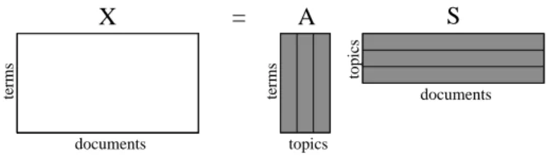
Hofmann’sprobabilistic latent semantic analysis (PLSA) [64, 65] is a strong matrix decom-position method for matrices of probabilities: P=AY. The decomposition resembles that of NMF except that all matrix entries have values between 0 and 1, and they sum to 1 at each column. PLSA is typically used in document analysis, with the aim of modeling the observed term and document frequencies by latent topics of discussion. The probability

P(i, j)of observing termiin documentj is presented as a convex combination of naspects

A(i, l), l = 1, . . . , n. The terms are conditionally independent given the topic. The model has the formp(W = w|D =d) = P

zp(Z =z|D =d)p(W =w|Z =z), whereZ, D and

W are random variables corresponding to the topics, documents and terms, respectively. In matrix form,P(i, j) givesp(W =wi|D=dj), A(i, l)givesp(W =wi|Z =zl)5 and Y(l, j)

givesp(Z =zl|D =dj). One main difference to NMF is that the probabilities P are not

observed, only the multinomial document vectors as columns ofX(an entry of a document vector gives the number of occurrences of a term in a document). The model is solved using the expectation-maximization (EM) algorithm [34].

Latent Dirichlet allocation(LDA) andmultinomial PCA(MPCA) as presented by [18], [102] and [20] are methods somewhat similar to Hofmann’s PLSA in that they are probabilistic in nature. In particular in MPCA, an observed document vector’s distribution is multinomial with a parameter vectorp=Ay. Herey, the proportions of different latent variables in this document, is first sampled from a Dirichlet distribution. The matrixAagain gives the prob-abilities of terms in different latent variables. For inference and learning in the LDA/MPCA model, a variational approximation of the data likelihood is done in [18], followed by an EM algorithm for maximum likelihood parameter estimation. Ways to enhance the estimation are presented by [102] and [20]. All of these approaches are computationally quite demand-ing. In a recent paper, Girolami and Kabán [52] have discussed the equivalence between PLSA and LDA.

A popular method for analyzing multidimensional data ismixture modeling where the ob-served data distribution is assumed to be a convex combination of some underlying latent distributions:p(x) =Pn

j=1πjpj(x|θj)whereπjis the probability that a data vectorxis

gen-erated by thejth component density pj with parametersθj; it also holdsPnj=1πj = 1. All

components xi of the observed vectorx have the same probabilities πj of being generated

by the jth underlying distribution. This is an important difference to ICA-type methods where the components xi of x may arise to different degrees A(i, j) from different latent

componentssj. In contrast to ICA, in mixture models it is also often assumed that one data

vector is generated by one latent distribution, although generation probabilities are given for all latent distributions. The observed vectors can then be clustered corresponding to

5

To be exact,p(W =wi|Z =zl) must be interpreted as the probability that topic zlgenerates word

wi; this is not the same as the probability of observingwi whenzl is active, as other topics thanzlmay

(26)

these latent distributions. Originally, the latent distributions were often assumed univariate Gaussian. In more recent papers, the observed data distribution is seen as a mixture of PCA’s [62], a mixture of probabilistic PCA’s [145], or a mixture of factor analyzers [49], to name a few; all of these are locally linear decompositions.

Local PCA[48] can be used in dimensionality reduction as discussed in [87]: the data space is first partitioned into disjoint regions, and PCA is then performed separately in each region. This approach is closely related to mixtures of PCA’s.

(27)

19

Chapter 3

ICA for complex valued signals

3.1 Introduction

The first theoretical development of ICA in this thesis is the separation of linearly mixed complex valued signals as presented in Publication 1. Here the problem is reviewed briefly and some new insights are given. The reader is referred to Publication 1 for more discussions and derivations.

A complex random variable z can be written as the sum of its real and imaginary parts, z=u+iv where uandv are real random variables. We denote byRe(z)the real part uof zand byIm(z)the imaginary partv ofz. Alternatively, a complex random variable can be presented in polar coordinates asz=ρeiφ _where_ρ_{is the modulus (also called radius) and}_φ

is the phase of the variable.

Complex valued signals are often encountered in, e.g., the fields of telecommunications or audio separation where convolutive (that is, time-lagged) signals are mixed: the sources are located so far away from the measurement locations that the source signals arrive at different instances in time, with possible echoes from nearby walls and so on. Moving into the frequency domain changes the convolution into multiplication, and an ICA-type mixing is obtained, where the mixtures, the sources and the mixing matrix are complex valued. A common practice is to divide the frequency domain into bins; this helps for example in noise cancellation, if colored noise is observed. Then a complex source separation task is solved in each bin. In the following section, an algorithm for the separation of complex valued signals is given.

3.2 A fast fixed-point algorithm

We assume that the ICA modelx=Asholds and both the independent component variables or source signalssand the observed variablesx are complex valued. The mixing matrixA

(28)

may be complex valued if desired. The source signals sj are assumed to have zero mean

and unit variance, with uncorrelated real and imaginary parts of equal variances. (The last assumption implies that sj must be strictly complex; the imaginary part may not vanish

everywhere.)

In the case of real valued signals, the independent components are typically found up to permutation and scaling. In the complex case, these indeterminacies hold as well, and in particular the scaling is complex valued. In other words, there is an unknown phase for each sj. This indeterminacy is an inherent property of complex ICA and not a consequence of

the assumptions made in our approach.

It will be assumed thatsj has a spherically symmetric distribution — thus the distribution

ofsjdepends on the modulus ofsj only and the scaling by a constant complex value does not

change the distribution ofsj. This assumption simplifies our approach and is quite realistic

in many applications, and it is also in line with the indeterminacy mentioned above. In Publication 1 a fast fixed point algorithm for the separation of complex valued signals is given. It is somewhat similar in nature to the FastICA algorithm [76, 70] briefly discussed in Section 2.2; hence the algorithm of Publication 1 is sometimes called the complex FastICA algorithm. The fixed-point algorithm for estimating one componenty=wHxis

w+ =E{x(wHx)∗g(|wHx_|2 )} −E{g(|wHx_|2 ) +|wHx_|2 g0(|wHx_|2 )}w (3.1) wnew= w+ ||w+_|| (3.2)

where the asterisk denotes complex conjugation, and wH is the vector w transposed and complex conjugated. The choice of the nonlinear function g is discussed in Publication 1. To estimate several components, the outputsw_jHxare decorrelated before the normalization (3.2) similarly to what was discussed in the end of Section 2.2. For details, please refer to Publication 1.

In Publication 1 we also give the conditions under which the estimator given by the algorithm is consistent.1

We start from an arbitrary nonlinear smooth contrast function and prove that its extrema coincide with the independent components. The nonlinear contrast function can be chosen quite freely to optimize, e.g., the statistical behavior of the estimator. This approach is computationally simple in contrast to another approach, where independence is measured by mutual information, approximated by cumulants. As discussed in Section 2.2, it is advisable to avoid cumulant nonlinearities as they are not robust against outliers in the data.

One practical implication of the consistency of the estimator is that the signs of the values of the contrast function for true independent components need not be known — in some ICA algorithms, the sign of the kurtosis (or some other function of the true sources) must be known.

Experimental results are given in Publication 1 to illustrate the performance of the fixed point algorithm and the theorem on the consistency of the estimator. Also, the connection

1

In the theorem on page 4 of the paper we assume thatG:R+_{∪ {}₀_{} →}

Ris a sufficiently smooth even

function. To be exact, there is a misprint here: the parity ofG is undetermined asG(y)only exists for

(29)

3.3. Random projection of complex signals 21

to independent subspace methods [75] and multidimensional ICA [23] is discussed: complex ICA is a restricted form of independent subspace methods.

Apart from the experimental results given in Publication 1, Fiori and Burrascano [45] com-pare the algorithm of Publication 1 with JADE [24] in electromagnetic source localization. No significant differences between the algorithms were found with respect to separation ac-curacy or computational complexity. Ristaniemi and Joutsensalo [128] use the algorithm of Publication 1 in separating the codes of different users in a CDMA (code-division multiple access) wireless communication network.

Earlier it was mentioned that the frequency domain is divided into bins and a complex ICA problem is solved in each bin. Due to the indeterminacy of the ordering of the estimated ICA components (similarly to the case of real valued signals) a permutation problem now arises: the order of the estimated sources should be the same in each bin. This problem is tackled in some of the references listed in Section 3.4.

3.3 Random projection of complex signals

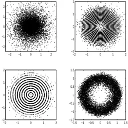
We next describe a small experiment on using random projection prior to ICA on high dimensional complex valued signals. The source signals are artificially generated complex random signalssj=ρjeiφj where for each signalj the modulusρj is drawn from a different

distribution (Exponential, Gamma, Poisson, Hypergeometric, Beta, Uniform, Weibull or Geometric) and the phaseφjis uniformly distributed on[−π, π]. The uniform phase ensures

that the distribution ofsj is spherically symmetric as discussed in Section 3.2. The sources

have unit variance. Examples of such source distributions are seen in Figure 3.1. The number of sources is 8, each having 50 000 observations. The sources are randomly mixed using a

(100×8)-dimensional complex valued mixing matrix.

The data described above are either random projected using a10×100-dimensional complex random matrix and then PCA preprocessed to 8 dimensions, or directly PCA preprocessed to 8 dimensions. The algorithm described in the previous section is then used to separate the sources, with a nonlinearityg(y) = 1/(2√ε+y)where ε= 0.1.

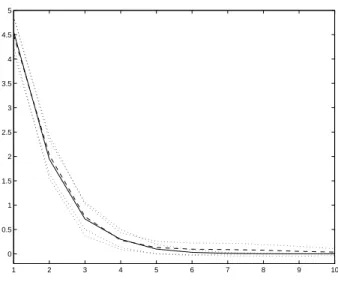
Similarly to the experiment in Section 2.3.2, we study the sums of squared errors (SSE) between the product of the mixing and unmixing matrices and a permutation matrix. Here the product matrix is transformed into the real domain by taking element-wise absolute values (remember from Section 3.2 that the sources are only estimated up to scaling by a complex unit-norm constant, so in the case of perfect separation, we get a permutation matrix with one unit-norm element in each row and each column). Figure 3.2 shows the average convergence of ICA estimation in the cases of random projected and original data, over 20 trials. We can see that both cases converge quickly and the SSE’s are almost equal.2 Thus at least in this small experiment, random projecting the high dimensional data prior to PCA preprocessing does not distort the data. Computing the random projection, PCA and ICA takes 77.3 seconds of CPU time on the average; directly computing PCA and then ICA

2

The 95 per cent confidence intervals over 20 trials are also plotted, although it is questionable whether the SSE’s are sufficiently Gaussian to permit the computation of the confidence intervals.

(30)

−2 −1 0 1 2 −2 −1 0 1 2 −2 −1 0 1 2 −2 −1 0 1 2 −2 −1 0 1 2 −2 −1 0 1 2 −1.5 −1 −0.5 0 0.5 1 1.5 −1.5 −1 −0.5 0 0.5 1 1.5

Figure 3.1: Examples of complex valued source signals with different modulus densities: Exponential (upper left), Poisson (upper right), Hypergeometric (lower left), Weibull (lower right). The source signals are spherically symmetric and have unit variance. The plane is the complex plane, the horizontal coordinate giving the real part and the vertical coordinate giving the imaginary part of a complex number.

takes 90.3 seconds of CPU time on the average3

. This shows that the preprocessing of data by random projection again gives computational savings. Also, the theorem on the local consistency of the estimator, discussed in Publication 1, is still applicable to the random projected data.

3.4 Other approaches

The separation of complex signals is already discussed in Comon’s seminal paper [29] from a cumulant point of view. The kurtosis of the estimated components is taken as a contrast function. In the complex case, kurtosis is not uniquely defined and its choice is discussed in [29]. The algorithm presented there is computationally quite demanding. A simpler algorithm is the cumulant-based JADE [25], also applicable to the complex case. Moreau and Macchi [105] give a cumulant-based algorithm which is also computationally heavy. A somewhat different but still cumulant-based approach is Back and Tsoi’s complex recur-rent network [8] that is analogous to Jutten and Herault’s algorithm [84]. Back and Tsoi’s algorithm is computationally somewhat demanding. The algorithm works partly in the time domain and partly in the frequency domain and they claim that the permutation problem between different frequency bins is thus overcome.

Comon and Moreau [31] give a cumulant-based algorithm for finding a sequence of Givens 3

Again, although computing the 95 per cent confidence intervals is a bit questionable, the interval is

(31)

3.4. Other approaches 23 1 2 3 4 5 6 7 8 9 10 0 0.5 1 1.5 2 2.5 3 3.5 4 4.5 5

Figure 3.2: Convergence of ICA estimation of complex valued signals. Horizontal axis: number of fixed point iterations. Vertical axis: Sum of squared errors of the estimated mixing matrix. Observation data are random projected prior to PCA preprocessing (solid line) or directly PCA preprocessed (dashed line). Dotted lines give 95 per cent confidence intervals over 20 trials.

complex rotations for 2-dimensional observations and an arbitrary number (≥2) of sources. Givens rotations [53] are used in some ICA algorithms in the real-valued case, too: The observed data are first whitened and dimensionality reduced so that only an orthogonal square mixing matrix is left to find. Any orthogonal m×m matrix can be written as a product of m(m−1)/2 Givens rotation matrices and a diagonal matrix with diagonal elements ±1. A Givens rotation is a plane rotation around the origin. The technique is useful in ICA in the two dimensional case but in higher dimensions several Givens rotations must be performed for each pair of components.

Smaragdis [140] presents a Bell-Sejnowski [13] type algorithm that is directly applicable to complex signals if transposes of vectors are simply changed to hermitians. An appropriate nonlinear function must be chosen: g(x) = tanh(x)used in the real case is unbounded in the complex domain, so he uses g(z) = tanh Re(z) +itanh Im(z). He proposes a heuristic coupling of adjacent frequency bins to make sure that the order of the estimated sources is the same in every frequency bin. The coupling approach is not always very effective, however. In the fields of speech and radar signal processing, a popular and robust approach to solving the permutation problem is direction of arrival estimation (see, e.g., [149, 150]). It is assumed that the spatial locations of sources with respect to the locations of measurement do not change. Each frequency band must have the same direction of arrival for a chosen source signal; this gives the correct ordering of the sources within frequency bands. Names such as beampattern analysis or null beamforming also refer to this technique.

Since the appearance of Publication 1, new approaches to complex signal separation have been discussed in the literature. These are briefly reviewed in the following.