San Ferm´ın: Aggregating Large Data Sets using a Binomial Swap Forest
†Justin Cappos and John H. Hartman
Department of Computer Science, University of Arizona
Abstract
San Ferm´ın is a system for aggregating large amounts of data from the nodes of large-scale distributed systems. Each San Ferm´ın node individually computes the aggre-gated result by swapping data with other nodes to dy-namically create its own binomial tree. Nodes that fall behind abort their trees, thereby reducing overhead. Hav-ing each node create its own binomial tree makes San Ferm´ın highly resilient to failures and ensures that the internal nodes of the tree have high capacity, thereby re-ducing completion time.
Compared to existing solutions, San Ferm´ın handles large aggregations better, has higher completeness when nodes fail, computes the result faster, and has better scal-ability. We analyze the completion time, completeness, and overhead of San Ferm´ın versus existing solutions using analytical models, simulation, and experimenta-tion with a prototype built on peer-to-peer system de-ployed on PlanetLab. Our evaluation shows that San Ferm´ın is scalable both in the number of nodes and in the aggregated data size. San Ferm´ın aggregates large amounts of data significantly faster than existing solu-tions: compared to SDIMS, an existing aggregation sys-tem, San Ferm´ın computes a 1MB result from 100 Plan-etLab nodes in 61–76% of the time and from 2-6 times as many nodes. Even if 10% of the nodes fail during ag-gregation, San Ferm´ın still includes the data from 97% of the nodes in the result and does so faster than the un-derlying peer-to-peer system recovers from failures.
1 Introduction
San Ferm´ın aggregates large amounts of data from dis-tributed nodes quickly and accurately. As disdis-tributed systems become more prevalent this is an increasingly important operation: for example, CERT logs about 1/4 TB of data daily on approximately 100 nodes distributed throughout the Internet [9]. Analysts use these logs to detect anomalous behavior that signals worms and other attacks, and must do so quickly to minimize damage. An example query might request the number of flows to and from each TCP/UDP port (to detect an anomalous dis-tribution of traffic indicating an attack). In this example there are many flow counters per node and the requester is interested in the sum of each counter across all nodes. It is important that the data be aggregated quickly, as time is of the essence when responding to attacks, and accu-rately, as the aggregated result should include data from
†This work was supported in part by the NSF under grant
CCR-0435292
as many nodes as possible and the data from each node exactly once. The more accurate the result, the more use-ful it is.
In San Ferm´ın the properties of current networks are leveraged to build an efficient content aggregation net-work for large data sizes. Since core bandwidth is typi-cally not the bottleneck [12], San Ferm´ın allows disjoint pairs of nodes to communicate simultaneously, as they will likely not compete for bandwidth. A San Ferm´ın node also sends and receives data simultaneously, mak-ing efficient use of full-duplex links. The result is that San Ferm´ın aggregates large data sets significantly faster than existing solutions, on average returning a 1 MB aggregation from 100 PlanetLab nodes in 61–76% the time and from approximately 2-6 times as many nodes as SDIMS, an existing aggregation system. San Ferm´ın is highly failure resistant and with 10% node failures dur-ing aggregation still includes the data from over 97% of the nodes in the result — and in most cases does so faster than the underlying peer-to-peer system recovers from failures.
San Ferm´ın uses abinomial swap forestto perform the aggregation, which is well-suited to tolerate failures and take advantage of the characteristics of the Internet. In a binomial swap forest each node creates its own binomial tree by repeatedly swapping aggregate data with other nodes. This makes San Ferm´ın highly resilient to failures because a particular node’s data is aggregated by an ex-ponentially increasing number of nodes as the aggrega-tion progresses. Similarly, the number of nodes included in a particular node’s aggregate data also increases expo-nentially as the aggregation progresses. Each node cre-ates its own binomial swap tree; as long as at least one node remains alive San Ferm´ın will produce a (possibly incomplete) aggregation result.
Having each node create its own binomial swap tree is highly fault-tolerant and fast, but it can lead to exces-sive overhead. San Ferm´ın reduces overhead by prun-ing small trees that fall behind larger trees durprun-ing the aggregation, as the small trees are unlikely to compute the result first and therefore increase overhead without improving speed or accuracy. When a tree falls behind San Ferm´ın prunes it — the name San Ferm´ın is derived from this behavior, after the festival with the running of the bulls in Pampalona.
1.1 Applications
In addition to CERT, San Ferm´ın also benefits other applications that aggregate large amounts of data from
many nodes:
Software DebuggingRecent work on software
debug-ging [19] leverages execution counts for individual structions. This work shows that the total of all the in-struction execution counts across multiple nodes helps the developer quickly identify bugs.
System Monitoring Administrators of distributed
systems must process the logs of thousands of nodes around the world to troubleshoot difficulties, track intru-sions, or monitor performance.
Distributed DatabasesA common query in relational
databases is GROUP BY [25]. This query combines ta-ble rows containing the same attribute value using an ag-gregate operator (such as SUM). The query result con-tains one table row per unique attribute value. In dis-tributed databases different nodes may store rows with the same attribute value. The values at these rows must be combined and returned to the requester.
These applications are similar because they aggregate large amounts of data from many nodes. For example, for the CERT example, finding the distribution of ports on UDP and TCP flows seen in the last hour takes 512 KB (assuming 4 byte counters). In the software debug-ging application, tracking a small application likebc quires 40KB of counters. Larger applications may re-quire more than 1MB of counters. The target environ-ments may contain hundreds or thousands of nodes, forc-ing the aggregation to tolerate failures.
The aggregation function has similar characteristics for these applications as well. The aggregation functions are commutative and associative but may be sensitive to duplication. Typically, the aggregate data from multiple nodes is approximately the same size as any individual node’s data.
The aggregation functions may also be sensitive to partial data in the result. If, for example, the data from a node is split and aggregated separately using different trees, the root may receive only some of the node’s data. For applications that want distributions of data (such as the target applications) it may be important to either have all of a node’s data or none of it.
In some cases it may be possible to compress aggre-gate data before transmission to reduce space. Such tech-niques are complimentary to this work. Some environ-ments may require administrative isolation. This work assumes that the aggregation occurs in a single adminis-trative domain with cooperative nodes.
2 Binomial Swap Forest
A binomial swap forest is a novel technique for aggre-gating data in which each node individually computes the aggregate result by repeatedly swapping (exchang-ing) aggregate data with other nodes. Two nodes swap data by sending each other the data they have aggregated
B A
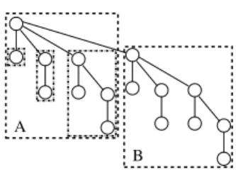
Figure 1: A 16-node binomial tree created by making tree B a child of tree A. The children of the root are themselves bino-mial trees of size 1, 2, 4, and 8.
D C D B A D C A B B A A B D C C
Figure 2: The binomial swap forest created by aggregating data from nodes A, B, C, and D. Each tree represents the sequence of swaps its root node performed while aggregating the data.
so far, allowing each to compute the aggregation of both nodes’ data. The swaps are organized so that a node only swaps with one other node at a time, and each swap roughly doubles the number of nodes whose data is in-cluded in a node’s aggregate data, so that the nodes will compute the aggregate result in roughlylog(N)swaps. If the nodes of the aggregation are represented as nodes in a graph, and swaps as edges in the graph, the sequence of swaps performed by a particular node form a bino-mial tree with that node at the root. As a reminder, in a binomial tree with2nnodes the children of the root are themselves binomial trees with2n−1,2n−2...,21, and20
nodes (Figure 1). As the figure illustrates, a binomial tree with2nnodes can be made from two binomial trees with
2n−1nodes by making one tree a child of the other tree’s root . The collection of binomial swap trees constructed by the nodes during a single aggregation is abinomial swap forest.
For example, consider data aggregation from four nodes: A, B, C, and D (Figure 2). Each node initially finds a partner with whom to swap data. Suppose A swaps with B and C swaps with D, so that afterwards A and B have the aggregate data AB, while C and D have the aggregate data CD. To complete the aggregation each node must swap data with a node from the other pair. If A swaps with C and B swaps with D, then every node will have the aggregate data ABCD .
The swaps must be carefully organized so that the se-ries of swaps by a node produces the correct aggregated result. Consider aggregating data fromN = 2n nodes each with a unique ID in the range[0..N −1](we will later relax these constraints). Since each swap doubles the amount of aggregate data a node has, just prior to the last swap a node must have the data from half of the
Nodes Lˆ2 Lˆ1 Lˆ0
000 Swap 001 Swap 010 Swap 101
001 Swap 000 Abort
010 N/A Swap 000 Swap 110
101 N/A Swap 110 Swap 000
110 Swap 111 Swap 101 Swap 010
111 Swap 110 Abort
Figure 3: One way 6 nodes can construct binomial swap forest.
Each node swaps data with a node in eachLkˆ starting withLmˆ
and ending withLˆ0.
101 110 111 111 110 110 011 001 000 111 101 110 000 000 110 011 001 000 001 011 101 000 001 101 111 111 001 011
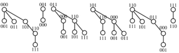
Figure 4: The binomial swap forest resulting from the construc-tion in Figure 3. Nodes 001 and 111 aborted.
nodes in the system, and must swap with a node that has the data from the other half of the nodes. This can be achieved by swapping based on node IDs; specifically, if the node ID for a nodexstarts with a 0 then node x
should aggregate data from all nodes that start with a 0 prior to the last swap, then swap with a nodey whose node ID starts with 1 that has aggregated data from all nodes that start with a 1. Note that it doesn’t matterwhich
nodeynodexswaps with as long as its node ID starts with a 1 and it has successfully aggregated data from its half of the node ID space. Also note that nodexshould swap with exactly one node from the other half of the ad-dress space, otherwise the result may contain duplicate data. Recursing on this idea, assuming that nodexstarts with 00 then in the penultimate swap it must swap with a node whose node ID starts with 01 thus aggregating data from all nodes that start with 0. Similarly, in the very first swap nodexswaps with the node whose node ID differs in only the least-significant bit. This is the general idea behind using a binomial swap forest to aggregate data — each node starts by swapping data with the node whose node ID differs in only the least-significant bit and works its way through the node ID space until it swaps with a node whose node ID differs in the most-significant bit.
Before describing this process in more detail it is use-ful to define thelongest common prefix,Lˆ of two nodes, which is the number of high-order bits the two node IDs have in common. We will use the notationL(x, y) =ˆ k
to mean that theLˆ of nodesxandyiskbits long. With respect to a particular nodex, we use the notationLˆxk to indicate the set of nodes whose longest common prefix with nodexiskbits long. We shorten this toLˆk when
it is clear which nodexis being referred to.
Using this notation, to aggregate data using a binomial
swap tree in a system withN = 2nnodes a nodexmust first swap data with a node inLˆxn−1 (there is only 1 node
in this set), then swap data with a node inLˆx
n−2, etc.,
until eventually swapping data with a node inLˆx0 (there are2n−1nodes in this set). Again, nodexswaps with only one node inLkˆ to prevent duplication in the result. Each setLˆx
k has2
n−k−1nodes, and nodexwill perform nswaps. Duplication cannot happen because when node
xswaps data with nodeyfrom setLˆx
k, nodexreceives
the data from nodes whose longest common prefix with node xis exactly k bits long. To see why this is true, consider that y has data from all nodes whose longest common prefix withyis at leastk+ 1bits. This means that the firstkbits of these nodes are the same asyand sincexdiffers withy in thekth bit,xmust differ with these nodes in thekth bit.
The discussion so far assumes that the number of nodes in the system is a power of 2, that node IDs are in the range [0..N −1], that each node knows how to contact every other node in the system directly, and that nodes do not fail. It also ignores the overhead of hav-ing each node construct its own binomial swap tree when only a single tree is necessary to compute the aggregated result. We can relax the first of these restrictions to allow the number of nodes to not be a power of 2, but it intro-duces several complications. First, the resulting binomial trees will not be complete, although they will produce the correct aggregate result. Consider data aggregation in a system with only nodes A, B, and C. Suppose A initially swaps with B. C must wait for A and B to finish swap-ping before it can swap with one of them. Suppose C subsequently swaps with A, so that both A and C have the aggregate data ABC, while node B only has AB. A and C successfully computed the result although the bi-nomial trees they constructed are not complete. B was unable to construct a tree containing all the nodes.
Second, some nodes may not be able to find partners with whom to swap, as is the case with node B in the previous example. More generally, consider a collection of nodes whose longest common prefixLˆiskbits long. To aggregate the data for that prefix the subset of nodes whoseLk+1ˆ ends with a 0 must swap data with the sub-set whoseLk+1ˆ ends with a 1. If these subsets are not of equal size, then some nodes will be unable to find a partner. Only ifN is a power of 2 can the two subsets have equal numbers of nodes, otherwise some nodes will be unable to find a partner and must abort their aggrega-tions.
Third, if the number of nodes is not a power of 2 then some node IDs will not be assigned to nodes. This can result in no nodes having a particular prefix, so that when other nodes try to swap with nodes having that prefix they cannot find a partner with whom to swap. Instead of aborting those nodes should instead simply skip the
pre-fix as it is empty. This is most likely to occur when the nodes initially start the aggregation process, as for any nodexLˆx
n corresponds to exactly one node ID, which may not be assigned to a node. Therefore, instead of starting the aggregation withLˆx
n nodexshould instead initially swap with a node inLˆx
m wheremis the longest prefix length for whichLˆx
m is not empty.
As an example of aggregating data when N is not a power of 2, suppose that there are 6 nodes: 000, 001, 010, 101, 110, and 111 (Figures 3 and 4). Each nodex swaps data with a node in eachLˆx
k starting withLˆxm and ending with Lˆx
0. There are many valid binomial swap
forests that could be constructed by these nodes aggre-gating data; in this example 000 first swaps with 001 and 110 swaps with 111. Lˆ2 is empty for 010 and 101, so
they swap with nodes inLˆ1: 000 swaps with 010 and 101
swaps with 111. 001 and 110 cannot find a node inLˆ1
with whom to swap (since 010 swapped with 000 and 101 swapped with with 111) and they stop aggregating data. In the final step the remaining nodes swap with a node inLˆ0: 000 swaps with 101 and 010 swaps with 111.
The swap operations in a binomial swap forest are only partially ordered – the only constraints are that nodes must swap with a node in each Lˆk in order starting withLˆm and ending withLˆ0. It is possible that in
Fig-ure 3 that nodes 000 and 010 will finish swapping before 111 and 110 finish swapping. This means that the only synchronization between nodes is when they swap data (there is no global synchronization between nodes).
San Ferm´ın makes use of an underlying peer-to-peer communication system to handle both gaps in the node ID space and nodes that are not able to communicate di-rectly. It uses time-outs to deal with node failures, and employs a pruning algorithm to reduce overhead by elim-inating unprofitable trees. Section 4 these aspects of San Ferm´ın in more detail.
3 Analytic Comparison
Several techniques have been proposed for content ag-gregation. The most straightforward is to have a single node retrieve all data and then aggregate. Some tech-niques like SDIMS [31] build a tree with high-degree nodes that are likely to have simultaneous connections. To provide resilience against failures, data is retransmit-ted when nodes fail. Seaweed [22] also has high-degree nodes with a similar structure to SDIMS, but uses a su-pernode approach in which the data on internal nodes are replicated to tolerate failures.
3.1 Analytic Models
Analytic models of these techniques enable comparison of their general characteristics. The models assume that any node that fails during the aggregation does not re-cover, and any node that comes online during the
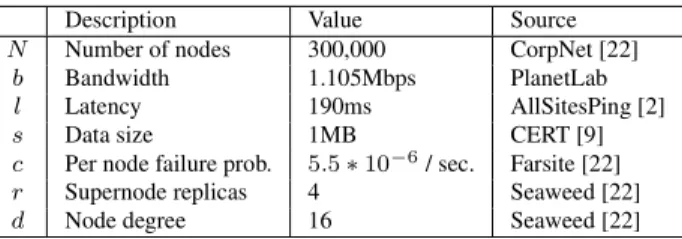
aggre-Description Value Source
N Number of nodes 300,000 CorpNet [22]
b Bandwidth 1.105Mbps PlanetLab
l Latency 190ms AllSitesPing [2]
s Data size 1MB CERT [9]
c Per node failure prob. 5.5∗10−6/ sec. Farsite [22] r Supernode replicas 4 Seaweed [22]
d Node degree 16 Seaweed [22]
Table 1: Model parameters.
gation does not join it. The probability of a given node failing in the next second isc. Node failures are assumed to be independent. A node that fails while sending data causes the partial data to be discarded. Inter-node laten-cies and bandwidths are a uniformlandb, respectively. The bandwidthb is per-node, which is consistent with the bandwidth bottleneck existing at the edges of the net-work and not in the middle. Each node contributes data of sizesand the aggregation function produces aggregate data of sizes. Per-packet, peer-to-peer, and connection establishment costs are ignored for all techniques.
Other parameters such as the amount of data aggre-gated, speed and capacity of the links, etc. are de-rived from real-world measurements (Table 1). The bandwidth measurements were gathered by transferring a 1MB file to all PlanetLab nodes from several well-connected nodes. The average bandwidth was within 100 Kbps for all runs, independent of the choice of source node. This means that well-connected nodes have roughly the same bandwidth to other nodes regardless of network location. The average of all runs is used in Ta-ble 1.
For each technique its completion time, completeness (number of nodes whose data is included in the aggregate result), and overhead are analyzed. Rather than isolating all of the parameters for each technique, the data size and number of nodes are varied to show their effect.
3.2 Binomial Swap Forest (San Ferm´ın)
The analysis of San Ferm´ın assumes a complete bino-mial swap forest. Since it takess
b +ltime to do a swap, the completion time islog2(N)∗(s
b +l). Figures 5a and 6a show that using a binomial swap forest is effec-tive at rapidly aggregating data. For example, using a binomial swap forest takes less than 1/3 the time of other techniques when more than 128 KB of data per node is aggregated.
After a node swaps withnother nodes in a binomial swap forest its data will appear in2n binomial trees, so that2nnodes must fail for the original node’s data to be lost. The probability of single node failing by timetis
1−(1−c)t, and the probability ofgnodes failing by time tis(1−(1−c)t)g. This leads to a completeness ofN−
Plog2(N) i=1 N 2∗(1−(1−c) i∗(s b+l))2 i−1 . As Figures 5b and 6b show, a binomial swap forest has high completeness
in the face of failures. For example, when aggregating more than 64KB of data, a binomial swap forest loses data from an order of magnitude fewer nodes than the other techniques.
Building a binomial swap forest involves each node swapping data with log2(N) other nodes. Assuming that failures do not impact overhead, the overhead is
N ∗ log2(N). As Figures 5c and 6c show, the over-head of a binomial swap forest is very high (Section 4 explains how San Ferm´ın reduces this overhead by prun-ing trees). Usprun-ing a binomial swap forest to aggregate 1MB of data requires about 20 times more overhead than balanced trees and about 5 times more than supernodes.
Intuitively, a binomial swap forest works well for two reasons. First, bandwidth dominates when aggregating large amounts of data. Other techniques build trees with higher fan-in so that nodes contend for bandwidth, while a binomial swap forest has no contention since swaps are done with only one node at a time. Second, data is replicated widely so that failures are less likely to reduce completeness. Nodes swap repeatedly, so that an expo-nential number of nodes need to fail for the data to be lost.
3.3 Centralized (Direct Retrieval)
In the centralized model, a central node contacts every node, retrieves their data directly, and computes the ag-gregated result. The central node can eliminate almost all latency costs by pipelining the retrievals, resulting in a completion time ofl+s∗Nb . This is much higher than the other techniques shown in Figure 5a because the time is linear in the number of nodes and the other techniques are logarithmic. As a result, to aggregate 1MB of data us-ing the centralized technique takes 26 days as compared to about 2 minutes with a binomial swap forest.
The completeness is the number of nodes that did not fail prior to the central node retrieving their data. The probability that a node is alive aftertseconds is(1−c)t,
so the expected completeness isPNi=1(1−c)i∗bs+l. As
can be seen in Figures 5b and 6b the centralized model has very poor results, despite assuming that the central node does not fail. The poor results are because many nodes fail before they are contacted by the central node.
The overhead is the number of nodes that were alive when contacted multiplied by the data size: PNi=1(1−
c)i∗bs+l∗N. A comparison is shown in Figures 5c and
6c. These results seem fantastic for large data sizes and numbers of nodes when compared to other algorithms, however what is really happening is that many nodes fail before their data is retrieved, reducing overhead but also reducing completeness.
3.4 Balanced Trees (SDIMS)
Aggregation is often performed using trees whose inter-nal nodes have similar degree dand whose leaf nodes have similar depth. An internal node waits for data from all of its children before computing the aggregated data and sending the aggregate result to its parent. In prac-tice, one of the child nodes is also the parent node so onlyd−1children send data to the parent. The model assumes that trees are balanced and complete with de-greed. If the effects of failures on completion time are ignored, the completion time islogd(N)∗((d−1)∗sb +l). As Figure 5a shows, this algorithm is quite fast when the data size is small and hence latency dominates. However, the performance quickly degrades when the data size in-creases. Aggregating 1MB of data using a balanced tree is about 4 times slower than using a binomial swap for-est.
A node that fails before sending to its parent will be missing from the result. It is also possible that both the child and parent fail after the child has sent the data, also causing the child to be missing. The completeness model captures these node failures. However, the model does not consider a cascade effect. This occurs when a par-ent has failed and another node is recovering the data from the children when a child fails. The node that covers and takes the role of the child would need to re-cover data from the child’s children. This is failure han-dling of a child within failure hanhan-dling of the parent (a cascade effect) and is not captured in the model. In the balanced tree model, there are N
(d−1)∗di nodes at level i. Since there is aPd−1j=1(1−(1−c)j∗s
b+l)
probabil-ity of an internal node failure withPi∗(d−1)k=1 (1−(1−
c)i∗((d−b1)∗s+l)+(k+j)∗s
b+l)probability of a
correspond-ing child failure, the balanced tree’s completeness is:
N−Plogd(N)−1 i=0 N (d−1)∗di∗ Pd−1 j=1(1−(1−c) j∗s b+l)∗ (1 +Pi∗(d−1)k=1 (1−(1−c)i∗((d−b1)∗s+l)+(k+j)∗ s b+l)). As
Figure 5b shows, the completeness is high when the ag-gregate data size is small. However, as the agag-gregate data size increases the completeness quickly falls off. When the number of nodes is varied instead (as in Figure 6b), the completeness is essentially the same as having ro-bust internal tree nodes that are provisioned against fail-ure. For example, with 1 million nodes it is expected that only 1% of the nodes that are excluded from the result are due to internal node failures. However, the high-degree nodes take a significant amount of time to receive the initial data from each node. The time the lowest level of internal nodes take to receive the initial data from their leaf node presents a significant time window for node failures. As a result using a binomial swap forest gives an order of magnitude improvement in completeness.
220 218 216 214 212 210 28 26 24 22 20 230 228 226 224 222 220 218 216 214 212 210 Co m pl et io n Ti m e (s ec on ds )
Data Size (bytes) Centralized
Binomial Balanced Supernode
(a) Completion Time vs. Data Size.
0 50000 100000 150000 200000 250000 300000 230 228 226 224 222 220 218 216 214 212 210 No de s M iss in g
Data Size (bytes) Centralized
Binomial Balanced Supernode
(b) Completeness vs. Data Size
234 232 230 228 226 224 222 220 218 216 214 212 210 230 228 226 224 222 220 218 216 214 212 210 By te s Se nt
Data size (bytes) Centralized
Binomial Balanced Supernode
(c) Overhead vs. Data Size
Figure 5: Scalability in the data size
0 200 400 600 800 1000 1200 1400 1600 1800 2000 220 218 216 214 212 210 28 26 24 Co m pl et io n Ti m e (s ec on ds ) Nodes Centralized Binomial Balanced Supernode
(a) Completion Time vs. Nodes
0 100 200 300 400 500 600 700 800 900 1000 220 218 216 214 212 210 28 26 24 No de s M iss in g Nodes Centralized Binomial Balanced Supernode (b) Completeness vs. Nodes 244 242 240 238 236 234 232 230 228 226 224 220 218 216 214 212 210 28 26 24 By te s Se nt Nodes Centralized Binomial Balanced Supernode (c) Overhead vs. Nodes
Figure 6: Scalability in the number of nodes
actually builds a binomial tree because internal nodes are counted as children at the lower levels. However, this is a single, static tree instead of a binomial swap for-est. This binomial tree still has roughly four times worse completeness than using a binomial swap forest. If the degree of the balanced tree were larger (such as 16 as is used in practice), the balanced tree would have even worse completeness.
In the balanced tree model, data is only sent multiple times when failures occur. There is a base cost of N
withPlogd(N)−1
i=0
N
(d−1)∗di nodes per level and a
proba-bility of failure of1−(1−c)(d−b1)∗s+lwith a
retrans-mission cost of approximately((i)∗(d−1)−1). The retransmission cost involves alld−1of the nodes at the priorinon-leaf levels retransmitting their aggregate data to their new parent (except the failed node). The over-head is therefore:s∗(N+Plogd(N)−1
i=0
N
(d−1)∗di∗1−(1−
c)(d−b1)∗s+l∗(i∗(d−1)−1)))which is very respectable
considering aggregate data is returned from most nodes. As Figures 5c and 6c show, the overhead is the lowest of the techniques with acceptable completeness. For exam-ple, when aggregating 1MB of data the overhead of bal-anced is about 4 times better than supernode and about 20 times better than using a binomial swap forest.
3.5 Supernode (Seaweed)
In this technique the nodes form a tree whose internal nodes replicate data before sending it up toward the root of the tree. Typically the tree is balanced and has uni-form degreed. To prevent the loss of data when an inter-nal node fails, there arerreplicas of each internal node. When a node receives data from a child it replicates the data before replying to the child. Ideally an internal node can replicate data from a child concurrently with receiv-ing data from another child. A node typically batches data before sending it to its parent to prevent sending small amounts of data through the tree.
The model allows internal nodes to replicate data while receiving new data, and assumes internal nodes send data to their parents as soon as they have received all data from their children. This means the model hides all but the initial delay in receiving the first bit of data (sb+l) in the replication time (r∗db∗s+ 2∗l) and leads to a com-pletion time oflogd(N)∗(s+rb∗d∗s+ 3∗l). However, the replication delay is significant as Figures 5a and 6a illustrate. Aggregating 1MB of data from 16 nodes using supernodes takes more than 8 minutes – about 16 times longer than it takes a binomial swap forest.
To simplify analysis the model assumes that there is enough replication to avoid losing all replicas of a su-pernode simultaneously. As a result, the only failures
that affect completeness are leaf nodes that fail before sending data to their parents. This leads to a complete-ness ofPdi=1Nd ∗(1−c)i∗(s
b)+l. As Figures 5b and 6b
show, this delay is enough to reduce the completeness below that of the binomial swap forest (by more than an order of magnitude when aggregating 1MB). This is because in a binomial swap forest the data is replicated to exponentially many nodes, while the supernode tech-nique has an initial significant window of vulnerability while the leaf nodes send their data to their parents.
The overhead is broken down into the cost of replicating data for internal nodes s ∗ (Nd−−1)1∗r, the cost of the leaf to internal node communication s ∗ (Pdi=1 r∗N∗(1−c)
i∗(sb+l)
d ), and the re-replication costs∗
(Pblogd(N)c−1 j=1
N
dj∗(1−(1−c)j
∗(r∗d∗bs+s+3∗l). As Fig-ures 5c and 6c show, the overhead of the supernode tech-nique is better than the binomial swap forest techtech-nique by about a factor of 4 but worse than the other techniques due to the supernode replication.
4 San Ferm´ın Details
This section describes the details of San Ferm´ın, includ-ing an overview of the Pastry peer-to-peer (p2p) message delivery subsystem used by the San Ferm´ın prototype, a description of how San Ferm´ın nodes find other nodes with whom to swap, how failures are handled, how time-outs are chosen, and how trees are pruned to minimize overhead.
4.1 Pastry
Pastry [26] is a peer-to-peer system similar to Chord [28] and Tapestry [35]. Each node has a unique 160-bit nodeId that is used to identify nodes and route messages. Given a message and a destination nodeId, Pastry routes the message to the node whose nodeId is numerically closest to the destination.
Each Pastry node has two routing structures: arouting tableand aleaf set. The leaf set for a node is a fixed num-ber of nodes that have the numerically closest nodeIds to that node. This assists nodes in the last step of routing messages and in rebuilding routing tables when nodes fail.
The routing table consists of node characteristics (such as IP address, latency information, and Pastry ID) orga-nized in rows by the length of the common prefix. When routing a message each node forwards it to the node in the routing table with the longest prefix in common with the destination nodeId.
Pastry uses nodes with nearby network proximity when constructing routing tables. As a result, the av-erage latency of Pastry messages is less than twice the IP delay [5]. For a complete description of Pastry see the paper by Rowstron and Druschel [26].
4.2 Overview
San Ferm´ın is part of a larger system for data aggrega-tion. Aggregation queries are disseminated to nodes us-ing SCRIBE [6] as the dissemination mechanism. These queries may either contain new code or references to ex-isting code that performs two functions: extraction and aggregation. The extraction function extracts the desired data from an individual node and makes it available for aggregation. For example, if the query is over flow data, the extraction function would open the flow data logs and extract the fields of interest.
The aggregation function aggregates data from mul-tiple nodes. This may be a simple operation like sum-ming data items in different locations or something more complex like performing object recognition by combin-ing data from multiple cameras.
When a node receives an aggregation request, the node disseminates the request and then runs the extraction function to obtain the data that should be aggregated. The San Ferm´ın algorithm is used to decide how the nodes should collaborate to aggregate data. San Ferm´ın uses the aggregation function provided in the aggregation request to aggregate data from multiple sources. Once a node has the result of the request it sends the data back to the requester. The requester then sends astop messageto all nodes (using SCRIBE) and they stop processing the request.
4.3 San Ferm´ın
There are several problems that must be solved for San Ferm´ın to work correctly and efficiently. First, a node must find other nodes with whom to swap aggregate data without complete information about the other nodes in the system. Second, a node must detect and handle the failures of other nodes. Third, a node must detect when the tree it is constructing is unlikely to be the first tree constructed and abort to reduce overhead. Each of these problems is addressed in the following subsections.
4.3.1 Finding Partners
To find nodes with whom to partner, each node first finds the longestLˆits Pastry nodeId has among all nodes. This is achieved by examining the nodeIds of the nodes in its leaf set. The node first swaps with a node that has the longestLˆ, then the second-longestLˆ, and so on, until the node swaps with a node that differs in the first bit. At this point the node has built a binomial tree with aggregate data from all nodes and has computed the result.
San Ferm´ın builds the binomial swap forest using a per-node prefix tablethat is constructed from node in-formation in Pastry’s routing table and leaf set. Theith row in the prefix table contains the nodes inLˆifrom the routing table and leaf set. Each node initially swaps with a node in the highest non-empty row in its prefix table,
then swaps with nodes in successive rows until culminat-ing with row 0. In this way San Ferm´ın approximates binomial trees. The nodeIds are randomly distributed, so
ˆ
Lp should contain about twice as many nodes asLˆp+1.
Since nodes swap aggregate data starting at their longest
ˆ
L, with each swap the number of nodes included in the aggregate data doubles. Swapping therefore doubles the number of nodes in the tree with each swap and thus ap-proximates a binomial tree.
Swapping is a powerful mechanism for aggregating data, but there are several issues that must be addressed. Pastry only provides each node with the nodeIds for a few nodes with eachLˆ, so how do nodes find partners with whom to swap? Also, how does a node know that another node is ready to swap with it? San Ferm´ın solves these problems usinginvitations, which are messages de-livered via Pastry that indicate that the sender is inter-ested in swapping data with the recipient. A node only tries to swap with another node if it has previously re-ceived an invitation from that node.
In addition to sending invitations to the nodes known by Pastry, invitations are also sent to random nodeIds with the correctLˆ. Pastry routes these invitations to the node with the nearest nodeId. This is important because Pastry will generally only know a subset of the nodes with a givenLˆ. To provide high completeness, a node in San Ferm´ın must find a live node with whom to swap with eachLˆ.
An empty row in the prefix table is handled differently depending on whether or not the associated Lˆk falls
within the node’s leaf set. IfLˆk is within the leaf set
thenLˆk must be empty because the Pastry leaf sets are
accurate. The node skips the empty row. Otherwise, if
ˆ
Lk is not within the leaf set, the node sends invitations
to random nodeIds inLˆk. If no nodes exist within theLˆk
the invitations will eventually time-out and the node will skipLˆk. This rarely happens, as the expected number of
nodes inLˆxincreases exponentially asxdecreases. As
an alternative to letting the invitations time-out, the the nodes that receive the randomly-sent messages could re-spond thatLˆk is empty. An emptyLˆkoutside of the leaf
set was never observed during testing so this modifica-tion is not necessary.
4.3.2 Handling Failures
Pastry provides a failure notification mechanism that al-lows nodes to detect other node failures, but it has two problems that make it unsuitable for use in San Ferm´ın. First, the polling rate for Pastry is 30 seconds, which can cause the failure of a single node to dominate the aggre-gation time. Second, some nodes that fail at the applica-tion level are still alive from Pastry’s perspective. A node may perform Pastry functions correctly, but have some other problem that prevents it from aggregating data.
For these reasons San Ferm´ın uses invitations to han-dle node failures, rather than relying exclusively on Pas-try’s failure notification mechanism. A node responds to an invitation to swap on a shorter Lˆ than its current
ˆ
Lwith a “maybe later” reply. This tells the sender that there is a live node with thisLˆthat may later swap with it. If a “maybe later” message is not received, the node sends invitations to random nodeIds with that Lˆ to try and locate a live node. If this fails, the node will eventu-ally conclude theLˆhas no live nodes and move on to the next shorterLˆ.
Since timeouts are used to bypass non-responsive nodes, selecting the proper timeout period for San Ferm´ın is important. Nodes may be overwhelmed if the timeout is too short and invitations are sent too fre-quently. Also short timeouts may cause nodes to be skipped during momentary network outages. If the time-out is too long then San Ferm´ın will recover from failures slowly, increasing completion time.
Rather than having a fixed timeout length for all val-ues of Lˆ, San Ferm´ın scales the timeout based on the estimated number of nodes with the value ofLˆ.Lˆvalues with more nodes have longer timeouts because it is less likely that all the nodes will fail. Conversely, Lˆ values with few nodes have shorter timeouts because it is more likely that all nodes will fail. In this case the node should quickly move on to the nextLˆ if it cannot contact a live node in the currentLˆ. A San Ferm´ın node estimates the number of nodes inLˆby estimating the density of nodes in the entire Pastry ring, which in turn is estimated from the density of nodes in its leaf set.
San Ferm´ın sets timeouts to be a small constantt mul-tiplied by the estimated number of nodes at Lˆ for the given value. This means that no matter how many nodes are waiting on a group of nodes, the nodes in this group will receive fewer than2∗tinvitations per second, on average. This timeout rate also keeps the overhead from invitations low.
4.3.3 Pruning Trees
Each San Ferm´ın node builds its own tree to improve per-formance and tolerate failures, but only one tree will win the race to compute the final result. If San Ferm´ın knew the winner in advance it could build only the winning tree and avoid the overhead of building the losing trees. Instead, San Ferm´ın builds all trees and prunes those un-likely to win. San Ferm´ın prunes a tree whenever its root node cannot find another node with whom to swap but there exists a live node with thatLˆ value. This is accom-plished by the use of “no” responses to invitations.
A node sends a “no” response to an invitation when its currentLˆis shorter than theLˆcontained in the invitation. This means the node receiving the invitation has already aggregated the data in the Lˆ and has no need to swap
with the node that sent the invitation. Whenever a node receives a “no” response it does not send future invita-tions to the node that sent the response. Unlike a “maybe later” response, “no” responses do not reset the timeout. If a node that has received a “no” response and it can-not find a partner for this value ofLˆ before the timeout expires, the node simply aborts its aggregation.
Note that a node will only receive a “no” response when two other nodes have its data in their aggregate data. This is because the node that sends a “no” response must have already aggregated data for thatLˆ(and there-fore must already have the inviting node’s data). Since the node that sent the “no” response has aggregated data for theLˆ via a swap then another node must also have the inviting node’s data.
4.3.4 San Ferm´ın Pseudocode
This section presents pseudocode for the San Ferm´ın al-gorithm, omitting details of error and timeout handling.
When a node receives a message: If message is an invitation:
If current ˆL shorter than ˆL in invitation reply with no
else reply with maybe_later and remember node that sent invitation
If message is a no, remember that one was received If message is a maybe_later then reset time-out If message is a stop then stop aggregation # Called to begin aggregation
Function aggregate_data(data, requester): Initialize the prefix_table from Pastry tables for ˆL in prefix_table from long to short:
Call aggregate_ˆL to swap data with a node If swap successful
compute aggregation of existing and received data Send aggregate data (the result) to the requester # A helper function to do aggregation for a value of ˆL Function aggregate_ˆL(data, known_nodes):
Try to swap data with nodes with this ˆL from whom an invitation was received
If successful then return the aggregate data
Send invitations to nodes in prefix table with this ˆL While waiting for a time-out:
If a node connects, swap with it and return the data Try to swap with nodes from whom we got invitations If success then return the aggregate data
# Time-out
if we got a no message, then stop (do not return) otherwise return no aggregate data
5 Evaluation
This section answers several questions about San Ferm´ın:
• How does San Ferm´ın compare to other existing so-lutions?
• How well does San Ferm´ın scale with the number of nodes and the data size?
• How well does San Ferm´ın tolerate failures?
• What is the overhead of San Ferm´ın?
• How effective is San Ferm´ın at utilizing high-capacity nodes?
5.1 Comparison
We developed a Java-based San Ferm´ın prototype that runs on the Java FreePastry implementation on Planet-Lab [23]. The SDIMS prototype (which also runs on FreePastry) was compared against San Ferm´ın in several experiments using randomly-selected live nodes with transitive connectivity and clock skew of less than 1 sec-ond. All experiments for a particular number of nodes used the same set of nodes.
The comparison with SDIMS demonstrates that ex-isting techniques are inadequate for aggregating large amounts of data. SDIMS was designed for streaming small amounts of data whereas San Ferm´ın is designed for one-shot queries of large amounts of data. Ideally, large SDIMS data would be treated as separate attributes and aggregated up separate trees. However, since this may include only part of a node’s data, this may skew the distribution of results returned. Therefore all data is aggregated as a single attribute.
One complication with comparing the two is zombie nodes in Pastry. San Ferm´ın uses timeouts to identify quickly nodes that are unresponsive. SDIMS however, relies on the underlying p2p network to identify unre-sponsive nodes, leaving it vulnerable to zombie nodes. After consulting with the SDIMS authors, we learned that they avoid this issue on PlanetLab by building more than one tree (typically four) and using the aggregate data from the first tree to respond. In the experiments we mea-sured SDIMS using both one tree (SDIMS-1) and four trees (SDIMS-4).
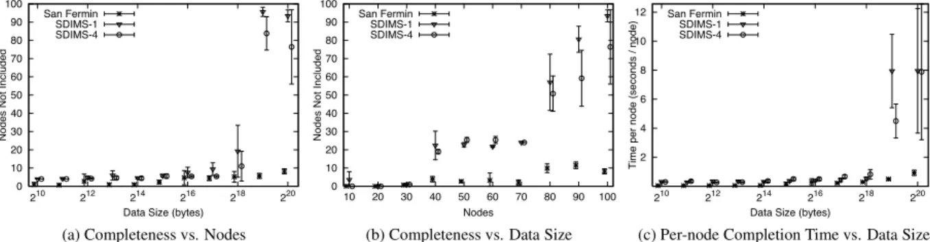
The experiments compare the time, overhead and completeness of SDIMS and San Ferm´ın. A small amount of accounting information was included in the aggregate data for determining which nodes’ data were included in the result. Unless specified otherwise, each experiment used 100 nodes and aggregated 1MB from each node, each data point is the average of 10 runs, and the error bars represent 1 standard deviation. All tests were limited to 5 minutes. In SDIMS the aggregate data trickles up to the root over time, so the SDIMS result was considered complete when either the aggregate data from all nodes reached the root or the aggregate data from at least half the nodes reached the root and no new data were received in 20 seconds.
Different aggregation functions such as summing counters, comparison for equals, maximum, and string parsing were experimented with. The choice of aggre-gation function did not have any noticeable effect on the experiments.
0 10 20 30 40 50 60 70 80 90 100 220 218 216 214 212 210 No de s No tI nc lu de d
Data Size (bytes) San Fermin
SDIMS-1 SDIMS-4
(a) Completeness vs. Nodes
0 10 20 30 40 50 60 70 80 90 100 10 20 30 40 50 60 70 80 90 100 No de s No tI nc lu de d Nodes San Fermin SDIMS-1 SDIMS-4
(b) Completeness vs. Data Size
12 10 8 6 4 2 220 218 216 214 212 210 Ti m e pe rn od e (s ec on ds /n od e)
Data Size (bytes) San Fermin
SDIMS-1 SDIMS-4
(c) Per-node Completion Time vs. Data Size
Figure 7: Comparison of San Ferm´ın and SDIMS on PlanetLab. SDIMS-1 is SDIMS using a single tree; SDIMS-4 is SDIMS using four trees.
5.1.1 Completeness
The first set of PlanetLab experiments measures com-pleteness as the aggregated data size increases (Fig-ure 7a). The number of nodes not included in the aggre-gate data is small for each algorithm until the data size exceeds 256KB. At that point SDIMS performs poorly because high-degree internal nodes are overwhelmed (shown in more detail in Section 5.4). San Ferm´ın con-tinues to include the aggregate data from most nodes.
The next set of experiments measures how the num-ber of nodes affects completeness (Figure 7b). When there are few nodes SDIMS-4 and San Ferm´ın algorithms do quite well. Once there are more than 30 nodes the SDIMS trees perform poorly due to high-degree internal nodes being overwhelmed with traffic.
5.1.2 Completion Time
Figure 7c shows per-node completion time, which is the completion time of the entire aggregation divided by the number of nodes whose data is included in the re-sult. This metric allows for meaningful comparisons be-tween San Ferm´ın and SDIMS because they may pro-duce results with different completeness. Data sizes larger than 256KB significantly increases the per-node completion time of SDIMS, while San Ferm´ın increases only slightly. Although not shown, for a given data size the number of nodes has little effect on the per-node com-pletion time.
Figure 8 illustrates the performance of individual ag-gregations in terms of both completion time and com-pleteness. Points near the origin have low completion time and high completeness, and are thus better than points farther away. San Ferm´ın’s points are clustered near the origin, indicating that it consistently provides high completeness and low completion time even in a dynamic environment like PlanetLab. SDIMS’s perfor-mance is highly variable — SDIMS-1 occasionally has very high completeness and low completion time, but more often performs poorly with more than half the
ag-0 10 20 30 40 50 60 70 80 90 100 300 250 200 150 100 50 0 No de s No tI nc lu de d
Completion Time (seconds)
San Fermin SDIMS-1 SDIMS-4
Figure 8: Completeness and Completion time of San Ferm´ın and SDIMS on PlanetLab. Each point represents a single run. Points near the origin are better because they have lower com-pletion time and higher completeness.
gregations missing at least 35 nodes from the result. SDIMS-4 performs even worse with all but 10 aggrega-tions missing at least 80 nodes.
5.2 Scalability
We used a simulator to measure the scalability of San Ferm´ın beyond that possible on PlanetLab. The sim-ulator is event-driven and based on measurements of real network topologies. Several simplifications were made to improve scalability and reduce the running time: global knowledge is used to construct the Pastry rout-ing tables; the connection teardown states of TCP are not modeled (as San Ferm´ın does not wait for TCP to com-plete the connection closure); and lossy network links are not modeled.
The simulations used network topologies from the University of Arizona’s Department of Computer Sci-ence (CS) and PlanetLab. The CS topology consists of a central switch connected to 142 systems with 1 Gbps links, 205 systems with 100 Mbps links, and 6 legacy systems with 10 Mbps links. Simulations using fewer nodes were constructed by randomly choosing nodes from the entire set.
The PlanetLab topology was derived from data pro-vided by theS3project [32]. The data provides pairwise
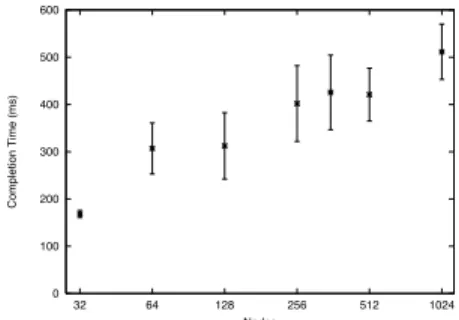
0 100 200 300 400 500 600 1024 512 256 128 64 32 Co m pl et io n Ti m e (m s) Nodes
Figure 9: Completion Time vs. Nodes, CS Topology.
0 100 200 300 400 500 600 220 218 216 214 212 210 Co m pl et io n Ti m e (m s)
Data Size (bytes)
Figure 10: Completion Time vs. Data Size, CS Topology. Each experiment used all 353 nodes.
latency and bandwidth measurements for all nodes on PlanetLab. Intra-site topologies were assumed to consist of a single switch connected to all nodes. The latency of an intra-site link was set to 1/2 of the minimum la-tency seen by the node on that link, and the bandwidth to the maximum bandwidth seen by the node. Inter-site latencies were set to the minimum latency between the two sites as reported byS3minus the intra-site latencies of the nodes. The inter-site bandwidths were set to the maximum bandwidths between the two sites.
In both topologies the Pastry nodeIds were randomly assigned, and a different random seed was used for each simulation. As in the PlanetLab experiments, unless specified otherwise, each experiment used 100 nodes and aggregated 1MB of data from each node, each data point is the average of 10 runs, and the error bars represent 1 standard deviation.
The first experiment varied the number of nodes in the system to demonstrate the scalability of San Ferm´ın; the results of the CS topology are shown in Figure 9. The completion time increases slightly as the number of nodes increases; when the number of nodes increases from 32 nodes to 1024 nodes the completion time only increases by about a factor of four. A 1024 node aggrega-tion of 1MB completed in under 500ms. The PlanetLab topology (not shown) has similar behavior — the com-pletion time also increases by approximately a factor of four as the number of nodes increases from 32 to 1024.
Figure 10 shows the result of varying the data size
100 90 80 70 60 50 40 30 20 10 0 0 10 20 30 40 50 Co m pl et io n Ti m e (s ec on ds ) Failures 0 1 5 15 30 60 inf
Figure 11: Completion Time vs. Failures, PlanetLab Topology. Each curve represents a different Pastry convergence time, from 0 seconds to infinity. 0 2 4 6 8 10 12 0 10 20 30 40 50 No de s No tI nc lu de d Failures CS Department PlanetLab
Figure 12: Completeness vs. Failures.
while using all 353 nodes in the CS topology. The com-pletion time is dominated by the p2p and message header overheads for data sizes under 128KB. When aggregat-ing more than 128KB the completion time increases sig-nificantly. The PlanetLab topology (not shown) has a similar pattern in which all of the data sizes under 128KB take about 4 seconds and thereafter the mean time in-creases linearly with the data size.
In all experiments the result included data from all nodes, therefore completeness results are not presented. 5.3 Failure Handling
The next set of simulations measured the effective-ness of San Ferm´ın at tolerating node failures. Failure traces were synthetically generated by randomly select-ing nodes to fail durselect-ing the aggregation. The times of the failures were chosen randomly from the start time of the aggregation to the original completion time. The p2p time to notice failures is varied to demonstrate the effect on San Ferm´ın.
The timeout mechanism in San Ferm´ın allows it to de-tect failures before the underlying p2p does. As a re-sult, the average completion time is less than the Pastry recovery time (Figure 11). On the PlanetLab topology, when the Pastry recovery time is less than 5 seconds, the cost of failures is negligible because other nodes use the time to aggregate the remaining data (leaving only failed subtrees to complete). When the recovery time is more than 5 seconds then some nodes end up timing-out
224 222 220 218 216 214 212 210 28 26 24 22 1024 512 256 128 64 32 Ne tw or k tra ffi c pe rn od e (b yt es ) Nodes CS p2p CS TCP PlanetLab p2p PlanetLab TCP
(a) Overhead vs. Nodes
224 222 220 218 216 214 212 210 28 26 24 22 220 218 216 214 212 210 Ne tw or k Tr af fic pe rn od e (b yt es )
Data Size (bytes) CS p2p
CS TCP PlanetLab p2p PlanetLab TCP
(b) Overhead vs. Data Size
0 100 200 300 400 500 600 700 800 220 218 216 214 212 210 To ta lB yt es Re ce ive d (M B)
Data Size (bytes) San Fermin
SDIMS-1 SDIMS-4
(c) Overhead Comparison
Figure 13: San Ferm´ın Overhead. Overhead is segregated into p2p and TCP traffic for (a) and (b).
a failed subtree before continuing. The CS department topology (not depicted) typically completes in less than 500ms so all non-zero Pastry recovery times increase the completion time. However, the average completion time is less than the Pastry recovery time for all recovery times greater than 1 second.
Figure 12 shows how failures affect completeness. Since failures occurred over the original aggregation time, altering the Pastry convergence time has little ef-fect on the completeness (and so the average of all runs is shown). The number of failures has different effects on the PlanetLab and CS topologies. There is greater variability of link bandwidths in the PlanetLab topol-ogy, which causes swaps to happen more slowly in some subtrees. Failures in those trees are more likely to de-crease completeness than in the CS topology, which has more uniform link bandwidths and the data swaps hap-pen more quickly. In both topologies the completeness is better than the number of nodes that failed — in most cases a node fails after enough swaps have occurred to ensure its data is included in the result.
5.4 Overhead
In this section two aspects of overhead are examined: the cost of invitations and the overhead characteristics as measured on PlanetLab. The two characteristics of in-terest are the total traffic during aggregation and the peak traffic observed by a node.
5.4.1 Overhead Composition
We ran simulations with varying numbers of nodes on the CS and PlanetLab network topologies to evaluate the composition of network traffic from San Ferm´ın (Fig-ure 13a). The traffic is segregated by type (p2p or TCP). The p2p traffic is essentially the traffic from invitations and responses while the TCP traffic is from nodes swap-ping aggregate data. The traffic per node does not sub-stantially increase as the number of nodes increases, meaning that the total traffic is roughly linear in the num-ber of nodes.
San Ferm´ın on the PlanetLab topology has higher p2p
and lower TCP traffic than on the CS topology. This is because PlanetLab’s latency is higher and more vari-able, causing the overall aggregation process to take much longer (which naturally increases the number of p2p messages sent). The PlanetLab bandwidth is also highly variable (especially intra-site links versus inter-site links). This causes high variability in partnering time, so that slow partnerings that might otherwise oc-cur do not because faster nodes have already computed the result.
As Figure 13a demonstrates, the p2p traffic is insignif-icant when 1MB of data is aggregated. Figure 13b shows how the composition of p2p and TCP traffic varies as the data size is varied. This is important for two reasons. First, it shows that the p2p traffic does not contribute sig-nificantly to the total overhead. Second, it shows how the total overhead varies with the data size. Doubling the data size caused the total overhead to roughly double.
Another notable result is that that the standard devia-tions were quite small, less than 4% in all cases. This makes it difficult to discern the error bars in the figures. 5.4.2 Total Traffic
The total network traffic of San Ferm´ın was also mea-sured experimentally on PlanetLab (Figure 13c). The re-sults from SDIMS are presented for comparison. For less than 256KB, SDIMS-1 incurs the least overhead, fol-lowed by San Ferm´ın and then SDIMS-4. After 256KB the overhead for SDIMS actually decreases because the completeness decreases. Nodes are overwhelmed by traffic and fail. A single internal node failure causes the loss of all data for it and its children until either the in-ternal node recovers or the underlying p2p network con-verges.
5.4.3 Peak Node Traffic
The peak traffic experienced by a node is important be-cause it can overload a node (Figure 14). To evaluate peak node traffic, an experiment was run on PlanetLab with 30 nodes aggregating 1 MB of data (30 nodes being
0 1 2 3 4 5 6 7 8 9 0 50 100 150 200 250 Tr af fic (M bp s) Time (seconds) Maximum SDIMS-1 Maximum SDIMS-4
Maximum San Fermin
San Fermin max SDIMS-1 max SDIMS-4 max
Figure 14: Peak Node Traffic. Each data point represents the peak traffic experienced by a node during that second of the aggregation.
the most nodes for which SDIMS had high complete-ness).
SDIMS internal nodes may receive data from many of their children simultaneously; the large initial peak of SDIMS traffic causes internal nodes that are not well-provisioned to either become zombies or fail. On the other hand, San Ferm´ın nodes only receive data from one partner at a time, reducing the maximum peak traffic. As a result, San Ferm´ın has a maximum peak node traffic that is less than 2/3 that of SDIMS.
5.5 Capacity
An important aspect of San Ferm´ın is that each node cre-ates its own binomial aggregation tree. By racing to com-pute the aggregate data, high-capacity nodes naturally fill the internal nodes of the binomial trees, while low-capacity nodes fill the leaves and ultimately prune their own aggregation trees.
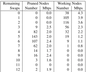
The final experiment measures how effective San Ferm´ın is at pruning low-capacity nodes. 1MB of data was aggregated from 100 PlanetLab nodes 10 times. The state of each node was recorded when the aggregation completed. Table 2 shows the results, including the num-ber of swaps remaining for each node to complete its ag-gregation and the average peak bandwidth of nodes with the same number of swaps remaining. Nodes with the higher capacity had fewer swaps remaining, whereas the nodes with lower capacity pruned their trees. The nodes in the middle tended to prune their trees but some were still working; the average peak bandwidth of these nodes was 2.1Mbps, whereas the average peak bandwidth of the nodes still working was 3.2Mbps. This means that nodes that are pruned have about 1/3 less observed ca-pacity than those nodes that are still aggregating data. This illustrates that San Ferm´ın is effective at having high-capacity nodes perform the aggregation and having low-capacity nodes prune their trees.
6 Related Work
Using trees to aggregate data from distributed nodes is not a new idea. The seminal work of Chang on
Remaining Pruned Nodes Working Nodes Swaps Number Mbps Number Mbps
0 0 0.0 38 4.3 1 0 0.0 105 3.9 2 0 0.0 116 3.6 3 9 2.5 56 2.3 4 82 2.0 32 2.2 5 143 2.0 19 1.2 6 107 2.4 9 1.1 7 62 2.0 1 0.8 8 14 1.7 0 0.0 9 16 2.4 0 0.0 10 3 1.6 0 0.0 11 0 0 0 0.0 12 2 1.9 0 0.0
Table 2: Effectiveness of San Ferm´ın at using high-capacity nodes. Thenumbercolumn is the number of nodes with the given number of swap remaining when the aggregation com-pleted; the Mbps column is the average peak bandwidth of those nodes.
Echo-Probe [7] formulated polling distant nodes and collecting data as a graph theory problem. More re-cently, Willow [30], SOMO [34], DASIS [1], Cone [3], SDIMS [31], Ganglia [21], and PRISM [15], have used trees to aggregate attributes Willow, SOMO, and Ganglia use one tree for all attributes, whereas SDIMS, Cone, and PRISM use one tree per attribute.
Seaweed [22] performs one-shot queries of small amounts of data and like San Ferm´ın is focused on com-pleteness. However, Seaweed trades completion time for completeness in that queries are expected to live for many hours or even days as nodes come online and re-turn aggregate data. Seaweed uses a supernode-based solution that further delays the timeliness of the initial aggregate data. Instead San Ferm´ın focuses on a differ-ent part of the design space, robustly returning aggregate data from existing nodes in a timely manner.
CONCAST [4] implements many-to-one channels as a network service. It uses routers to aggregate data over a single tree. As the size of the aggregate data grows the memory and processing requirements on routers be-comes prohibitive.
Gossip and epidemic protocols have also been used for aggregation [18, 13, 17, 16], including Astrolabe [29]. Unstructured protocols that rely on random exchanges face a trade-off between precision and scalability. Struc-tured protocols, such as Astrolabe, impose a structure on the data exchanges that prevents duplication. This is at the cost of creating and maintaining a structure, and con-fining the data exchanges to adhere to the structure.
Data aggregation is also an issue in sensor net-works. Unlike San Ferm´ın, the major concerns in sen-sor networks are power consumption and network traf-fic. Examples of data aggregation in sensor networks are
TAG [20], Hourglass [27], and Cougar [33].
Distributed query processing involves answering queries across a set of distributed nodes. The most rele-vant to our work are systems such as PIER [14], which stores tuples in a DHT as part of processing a query. Dis-tributed query processing also encompasses performing queries on continuous streams of data, as is done in Au-rora [8], Medusa [8], and HiFi [11].
There are several systems that have focused on aggre-gating data from large data sets from a programming lan-guage perspective [10, 24]. However neither system fo-cuses on sending large amounts data over the network.
7 Conclusions
This paper presents San Ferm´ın, a technique for ag-gregating large amounts of data that when agag-gregating 1MB of data provides 2-6 times better completeness than SDIMS, at 61-76% of the completion time, and with bet-ter scalability characbet-teristics. San Ferm´ın has a peak node traffic more than 1/3 lower than that of SDIMS, which accounts for much of the higher completeness. Our analysis shows that when 10% of the nodes fail dur-ing aggregation San Ferm´ın still computes the aggre-gated result from 97% of the nodes. San Ferm´ın also scales well with the number of nodes or the data size – completion time increases by less than a factor of 4 if the number of nodes increases from 32 to 1024, and by about a factor of 2 as the data size increases from 256KB to 1MB.
Acknowledgments
We would like to thank the SDIMS group (especially Navendu Jain) for helping us use and evaluate SDIMS. We would especially like to thank our shepherd Arun Venkataramani and the anonymous reviewers for their helpful feedback.
References
[1] K. Albrecht, R. Arnold, M. G¨ahwiler, and R. Wattenhofer. Ag-gregating information in peer-to-peer systems for improved join and leave. InPeer-to-Peer Computing, 2004.
[2] PlanetLab - All Sites Ping. http://ping.ececs.uc.edu/ping/.
[3] R. Bhagwan, G. Varghese, and G. Voelker. Cone: Augmenting DHTs to support distributed resource discovery. Technical Report CS2003-0755, UCSD, 2003.
[4] K. Calvert, J. Griffioen, B. Mullins, A. Sehgal, and S. Wen. Con-cast: design and implementation of an active network service. IEEE JSAC, 19(3), 2001.
[5] M. Castro, P. Druschel, Y. Hu, and A. Rowstron. Exploiting net-work proximity in distributed hash tables. InFuDiCo, 2002. [6] M. Castro, P. Druschel, A. Kermarrec, and A. Rowstron.
SCRIBE: A large-scale and decentralized application-level mul-ticast infrastructure.IEEE JSAC, 20(8), 2002.
[7] E. J. H. Chang. Echo algorithms: Depth parallel operations on general graphs.IEEE TSE, 1982.
[8] M. Cherniack, H. Balakrishnan, M. Balazinska, D. Carney, U. C¸ etintemel, Y. Xing, and S. B. Zdonik. Scalable distributed stream processing. InCIDR, 2003.
[9] M. Collins. Personal correspondance, Sept. 2006.
[10] J. Dean and S. Ghemawat. MapReduce: Simplified data process-ing on large clusters. InOSDI, 2004.
[11] M. J. Franklin, S. R. Jeffery, S. Krishnamurthy, F. Reiss, S. Rizvi, E. Wu, O. Cooper, A. Edakkunni, and W. Hong. Design consid-erations for high fan-in systems: The HiFi approach. InCIDR, pages 290–304, 2005.
[12] J. Guicahrd, F. le Faucheur, and J. P. Vasseur. Definitive MPLS Network Designs. Cisco Press, 2005.
[13] I. Gupta, R. van Renesse, and K. P. Birman. Scalable fault-tolerant aggregation in large process groups. InIEEE DSN, 2001. [14] R. Huebsch, J. M. Hellerstein, N. Lanham, B. T. Loo, S. Shenker, and I. Stoica. Querying the Internet with PIER. InVLDB, 2003. [15] N. Jain, D. Kit, D. Mahajan, M. Dahlin, and Y. Zhang. PRISM:
Precision integrated scalable monitoring. Technical Report TR-06-22, University of Texas, Feb. 2006.
[16] M. Jelasity, W. Kowalczyk, and M. van Steen. An approach to massively distributed aggregate computing on peer-to-peer net-works. InEuromicro Conference on Parallel, Distributed and Network-Based Processing, 2004.
[17] M. Jelasity and A. Montresor. Epidemic-style proactive aggrega-tion in large overlay networks. InICDCS, 2004.
[18] M. Jelasity, A. Montresor, and O. Babaoglu. Gossip-based aggre-gation in large dynamic networks. ACM TOCS, 23(3):219–252, 2005.
[19] B. R. Liblit. Cooperative Bug Isolation. PhD thesis, University of California, Berkeley, Dec. 2004.
[20] S. Madden, M. J. Franklin, J. M. Hellerstein, and W. Hong. TAG: A Tiny AGgregation service for ad-hoc sensor networks. In OSDI, 2002.
[21] M. L. Massie, B. N. Chun, and D. E. Culler. The Ganglia dis-tributed monitoring system: design, implementation, and experi-ence.Parallel Computing, 30(7), July 2004.
[22] D. Narayanan, A. Donnelly, R. Mortier, and A. Rowstron. Delay aware querying with Seaweed. InVLDB, 2006.
[23] L. Peterson, D. Culler, T. Anderson, and T. Roscoe. A blueprint for introducing disruptive technology into the Internet. In Hot-Nets, 2002.
[24] R. Pike, S. Dorward, R. Griesemer, and S. Quinlan. Interpreting the data: Parallel analysis with Sawzall.Scientific Programming, 13(4):277–298, 2005.
[25] R. Ramakrishnan and J. Gehrke.Database Management Systems. McGraw-Hill Higher Education, 2000.
[26] A. Rowstron and P. Druschel. Pastry: Scalable, decentralized object location, and routing for large-scale peer-to-peer systems. InICDCS, 2001.
[27] J. Shneidman, P. Pietzuch, J. Ledlie, M. Roussopoulos, M. Seltzer, and M. Welsh. Hourglass: An infrastructure for con-necting sensor networks and applications. Technical Report TR-21-04, Harvard University, 2004.
[28] I. Stoica, R. Morris, D. Karger, F. Kaashoek, and H. Balakrish-nan. Chord: A scalable Peer-To-Peer lookup service for Internet applications. InSIGCOMM, 2001.
[29] R. van Renesse and K. Birman. Astrolabe: A robust and scalable technology for distributed system monitoring, management, and data mining.ACM TOCS, May 2003.
[30] R. van Renesse and A. Bozdog. Willow: DHT, aggregation, and publish/subscribe in one protocol. InInternational Workshop on Peer-to-Peer Systems (IPTPS), 2004.
[31] P. Yalagandula and M. Dahlin. A scalable distributed information management system. InSIGCOMM, 2004.
[32] P. Yalagandula, P. Sharma, S. Banerjee, S. Basu, and S.-J. Lee. S3: a scalable sensing service for monitoring large networked systems. InSIGCOMM workshop on Internet network manage-ment, 2006.
[33] Y. Yao and J. Gehrke. The Cougar approach to in-network query processing in sensor networks. SIGMOD, 31(3):9–18, Sept. 2002.
[34] Z. Zhang, S.-M. Shi, and J. Zhu. SOMO: Self-organized metadata overlay for resource management in P2P DHT. InInternational Workshop on Peer-to-Peer Systems (IPTPS), 2003.
[35] B. Zhao, L. Huang, J. Stribling, S. Rhea, A. Joseph, and J. Ku-biatowicz. Tapestry: a resilient global-scale overlay for service deployment.IEEE JSAC, 2003.