Feedback Control for Adaptive Live Video Streaming

(1)

Feedback Control for Adaptive Live Video Streaming

Luca De Cicco

Politecnico di Bari Bari, Italy

Saverio Mascolo

Vittorio Palmisano

ABSTRACT

Multimedia content feeds an ever increasing fraction of the Internet traffic. Video streaming is one of the most impor-tant applications driving this trend. Adaptive video stream-ing is a relevant advancement with respect to classic pro-gressive download streaming such as the one employed by YouTube. It consists in dynamically adapting the content bitrate in order to provide the maximum Quality of Experi-ence, given the current available bandwidth, while ensuring a continuous reproduction. In this paper we propose a Qual-ity Adaptation Controller (QAC) for live adaptive video streaming designed by employing feedback control theory. An experimental comparison with Akamai adaptive video streaming has been carried out. We have found the fol-lowing main results: 1) QAC is able to throttle the video quality to match the available bandwidth with a transient of less than 30s while ensuring a continuous video repro-duction; 2) QAC fairly shares the available bandwidth both in the cases of a concurrent TCP greedy connection or a concurrent video streaming flow; 3) Akamai underutilizes the available bandwidth due to the conservativeness of its heuristic algorithm; moreover, when abrupt available band-width reductions occur, the video reproduction is affected by interruptions.

Categories and Subject Descriptors

C.2.5 [Local and Wide-Area Networks]: Internet; H.5.1 [Multimedia Information Systems]: Video

General Terms

Design, Performance, Experimentation

Keywords

Adaptive Video Streaming, quality feedback control, quality adaptation controller

Permission to make digital or hard copies of all or part of this work for personal or classroom use is granted without fee provided that copies are not made or distributed for profit or commercial advantage and that copies bear this notice and the full citation on the first page. To copy otherwise, to republish, to post on servers or to redistribute to lists, requires prior specific permission and/or a fee.

1. INTRODUCTION

Nowadays, the wide availability of wired and wireless broad-band connections is enabling ubiquitous multimedia appli-cations over the Internet, such as video streaming, personal video broadcasting, IPTV, and videoconferencing, at video resolutions that can scale up to full high definition (full HD, 1920x1080) at frame rates up to 30 fps. Such rich video contents require a compressed bitstream in the order of 10 Mbps along with adequate processing resources at the client for decoding. Nevertheless, the Internet is becoming more and more accessible to a wide spectrum of devices: if desk-tops users are normally equipped with large screens, good processing resources, and wired broadband connections, mo-bile users typically use small screens devices, with limited processing resources and wireless cellular connections that are characterized by variable link characteristics.

Thus, a key challenge is to provide the user with a seam-less multimedia experience at the maximum Quality of Ex-perience (QoE) that can be obtained given the available de-vice and network resources. To this purpose, multimedia content must be made adaptive. It is important to notice that the adaptation process should account take into ac-count a wide set of variables such as user screen resolution, CPU load, network available bandwidth, power consump-tion, some of which are time-varying. In this paper we focus on adaptation to network available bandwidth.

Adaptive (live) video streaming represents a relevant ad-vancementwrt classic progressive download streaming such as the one employed by YouTube.

In classicprogressive download streaming, the video is de-livered as any data file using greedy TCP connections. The video stream is buffered at the receiver for a while before the playing is started so that short-term mismatches be-tween the video bitrate and the available network bandwidth can be absorbed and video interruptions could be mitigated. Nevertheless, if the mismatch persists the buffer could even-tually get empty and playback interruptions could occur af-fecting the user experience.

On the other hand, with adaptive streaming the video source is adapted on-the-fly so that the user can watch videos at the maximum bitrate that is allowed by the time-varying available bandwidth and by the device resources.

In this paper we focus on a particular adaptive stream-ing approach that is the stream-switching technique: the server encodes the video content at different bitrates and it switches from one video version to another based on client feedbacks such as the measured available bandwidth. This approach is employed by Apple HTTP live streaming,

(2)

Mi-crosoft IIS server, Adobe Dynamic Streaming, Akamai HD Video Streaming, and Move Networks. In particular, we present a Quality Adaptation Controller (QAC), which has been designed using feedback control, to drive stream-switching for adaptive live streaming applications. The advantages of using a control theoretical approach to design the controller as opposed to a heuristic-based design is a cleaner design that can be not only experimentally tested but also mathe-matically analyzed.

The rest of the paper is organized as follows: Section 2 provides a brief review of the different adaptive streaming al-gorithms proposed in the literature along with the main fea-tures of the adaptive streaming algorithms employed in com-mercial products; Section 3 summarizes the results obtained by an experimental investigation of Akamai HD Video Stream-ing; in Section 4 we propose the Quality Adaptation Con-troller (QAC) and in Section 5 we experimentally compare QAC with the Akamai HD Video Streaming; finally, Section 6 concludes the paper.

2. RELATED WORKS

In this Section we provide a review of the relevant litera-ture on adaptive streaming and then we focus on the most known commercial products providing adaptive streaming services.

2.1 Adaptive streaming techniques

In the last decade a vast literature on video streaming has been produced. Main topics that have been investigated are: 1) the design of transport protocols specifically tailored for video streaming, 2) adaptation techniques, 3) scalable codecs.

Concerning the first topic, several transport protocols de-signed for video streaming have been proposed, such as the TCP Friendly Rate Control (TFRC) [7], Real Time Stream-ing Protocol (RTSP) [14], Microsoft Media Services (MMS), Real Time Messaging Protocol (RTMP) [3]. Some of the mentioned protocols have been employed in commercial prod-ucts such as RealNetworks, Windows Media Player, Flash Player. Even though TCP has been regarded in the past as inappropriate for the transport of video streaming proto-cols, recently it is getting a wider acceptance and it is being used with the HTTP. This is mainly due to the following reasons: i) Internet applications are rapidly converging on web browsers; ii) HTTP-based streaming is cheaper to de-ploy since it emde-ploys standard HTTP servers [17]; iii) TCP has built-in NAT traversal functionalities; iv) it is easy to be deployed within Content Delivery Networks (CDN) [17]; v) TCP delivers most part of the Internet traffic and it is able to guarantee the stability of the network by means of an efficient congestion control algorithm [15].

In [16] the authors develop analytic performance mod-els to assess the performance of TCP when used to trans-port a live video streaming source without the use of quality adaptation. The theoretical results, obtained considering a constant bit rate (CBR) source and supported by an ex-perimental evaluation, suggest that in order to achieve good performance in terms of startup delay and percentage of late packet arrivals, TCP requires a network bandwidth that is roughly two times the video bit rate. It is important to stress that such bandwidth over-provisioning would systematically waste half of the available bandwidth.

For what concerns adaptation techniques, different

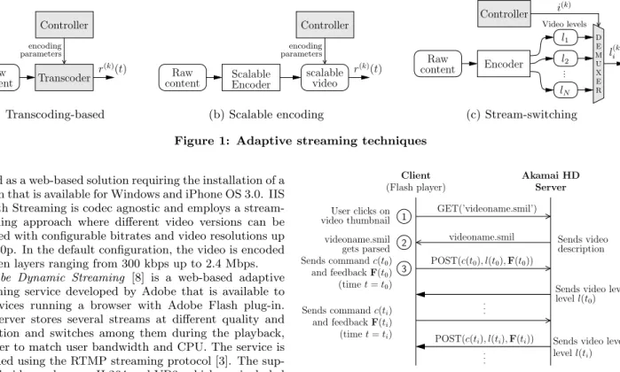
ap-proaches have been proposed in the literature so far. The issue here is how to automatically throttle the video quality to match the available resources (network bandwidth, CPU) so that the user receives the video at the maximum possible quality. The proposed techniques to adapt the video source bitrate to the variable bandwidth can be classified into three main categories: 1) transcoding-based, 2) scalable encoding-based, 3) stream-switching (or multiple-bitrate - MBR). Fig-ure 1 shows a schematic representation of each considered technique. In the figure, the blocks represented in gray are those requiring on-the-fly per-client processing and the (k) index refers to variables pertaining to thek-th client access-ing the same video content. In particular, encoders can be considered as the most CPU-consuming function, whereas controllers generally require much less processing capacity.

The transcoding-based [12] approach (see Figure 1(a)), consists in adapting the video content to match a specific bitrate by means of on-the-fly transcoding of the raw con-tent. These algorithms can achieve a very fine granularity by throttling frame rate, compression, and video resolution. Nevertheless, this comes at the cost of increased processing load and poor scalability, due to the fact that transcoding has to be done on a per-client basis. Another important issue is that such algorithms are difficult to be deployed in CDNs.

Another important class of adaptation algorithms (see Figure 1(b)) employsscalable codecssuch as H264/MPEG-4 AVC [9, 10]. Both spatial and temporal scalability can be exploited to adapt picture resolution and frame rate without having to re-encode the raw video content. With respect to transcoding-based approach, scalable codecs reduce process-ing costs since the raw video is encoded once and adapted on-the-fly by exploiting the scalability features of the en-coder. To be used with CDNs, this approach requires spe-cialized servers implementing the adaptation logic. Also this approach is difficult to be used with CDNs since the adap-tation logic requires to be run on specialized servers and content cannot be cached in standard proxies. Another is-sue is that the adaptation logic depends on the employed codec, thus restricting the content provider to use only a limited set of codecs.

Stream-switchingalgorithms (see Figure 1(c)) encode the raw video content at increasing bitrates resulting into N

versions, i.e. video levels; an algorithm dynamically chooses the video level that matches the user’s available bandwidth; those algorithms minimize the processing costs since, once the video is encoded, no further processing is required in order to adapt the video to the variable bandwidth [17, 1, 11, 2, 8]. Another important advantage of such algorithms is that they do not rely on particular functionalities of the employed codec and thus can be made codec-agnostic. The disadvantages of this approach are the increased storage re-quirements and the fact that adaptation is characterized by a coarser granularity since video bitrates can only belong to a discrete set of levels.

2.2 Stream-switching adaptive video

stream-ing commercial products

Stream-switching, or Multiple Bit-Rate (MBR) stream-ing, is gaining momentum since leading commercial media players are preferring it to the other streaming approaches.

IIS Smooth Streaming [17] is a live adaptive streaming service provided by Microsoft. The streaming technology is

(3)

Raw content Transcoder encoding parameters r(k)₍_t₎ Controller (a) Transcoding-based Raw content scalable video encoding parameters Scalable Encoder r(k)₍_t₎ Controller (b) Scalable encoding Raw content E M U D X E R l1 l2 lN Video levels Encoder i(k) l(ik) Controller (c) Stream-switching

Figure 1: Adaptive streaming techniques

offered as a web-based solution requiring the installation of a plug-in that is available for Windows and iPhone OS 3.0. IIS Smooth Streaming is codec agnostic and employs a stream-switching approach where different video versions can be encoded with configurable bitrates and video resolutions up to 1080p. In the default configuration, the video is encoded in seven layers ranging from 300 kbps up to 2.4 Mbps.

Adobe Dynamic Streaming [8] is a web-based adaptive streaming service developed by Adobe that is available to all devices running a browser with Adobe Flash plug-in. The server stores several streams at different quality and resolution and switches among them during the playback, in order to match user bandwidth and CPU. The service is provided using the RTMP streaming protocol [3]. The sup-ported video codecs are H.264 and VP6, which are included in the Adobe Flash plug-in.

Apple has recently released a client-sideHTTP Adaptive Live Streamingsolution [11]. The server segments the video content into several pieces with configurable duration and video quality. The server exposes a playlist (.m3u8) con-taining all the available video segments. The client down-loads consecutive video segments and it dynamically chooses the video quality by using an undisclosed algorithm. Apple HTTP Live Streaming employs H.264 codec using a MPEG-2 TS container and it is available on any device running iPhone OS 3.0 or later (including iPad), or any computer with QuickTime X or later installed.

Move Networks provides live adaptive streaming service to several TV networks such as ABC, FOX, Televisa, ESPN and others. A plug-in, available for the most used web browsers (Windows and Mac OS X) has to be installed to access the service. Move Networks employs VP7, a video codec developed by On2, a company that has been recently acquired by Google. Adaptivity to available bandwidth is provided using the stream-switching approach. Five differ-ent versions of the same video are available at the server with bitrates ranging from 100 kbps up to 2200 kbps.

Hulu1offers on demand TV shows and movies in the USA. In 2010 Hulu has launched a new video player that im-plements adaptivity by employing the stream-switching ap-proach. The adaptation algorithm does not change the video frame rate, whereas it sets the video resolution to match the current user available bandwidth.

3. AKAMAI ADAPTIVE STREAMING

In this Section we summarize and significantly extend the results obtained in a recent experimental investigation of the Akamai HD Video Streaming (AHDVS) service [5].

1 http://www.hulu.com 1 2 3 Client

(Flash player) Server

Akamai HD GET(’videoname.smil’) User clicks on video thumbnail videoname.smil gets parsed POST(c(t0), l(t0),F(t0)) Sends video description Sends commandc(t0) and feedbackF(t0) (timet=t0) videoname.smil

Sends video level levell(t0)

Sends commandc(ti)

and feedbackF(ti)

(timet=ti)

Sends video level levell(ti)

POST(c(ti), l(ti),F(ti))

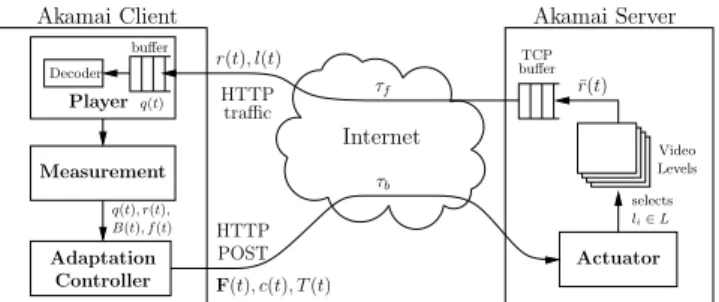
Figure 2: Client-server time sequence graph: thick lines represent video data transfer, thin lines repre-sent HTTP requests repre-sent from client to server

3.1 Client-server protocol

AHDVS employs HTTP connections to stream data from the server to the client. The adaptation algorithm is exe-cuted at the client in a Flash application. By analyzing the traffic between the Akamai server and the client we have ob-served that the client issues a number of HTTP requests to the server throughout all the duration of the video stream-ing. Figure 2 shows a typical time sequence graph of the HTTP requests sent from the client to the Akamai server.

At first, the client connects to the Akamai server [1], then a Flash application is loaded and a number of videos are made available to the client. When the user clicks on the thumbnail (1) of the video he is willing to play, a GET HTTP request is sent to the server which points to a SMIL2

compliant file. In the SMIL file the base URL of the video, the available video levels, and the corresponding encoding bit-rates are provided.

After that, the client parses the SMIL file (2) to recon-struct the complete URLs of the available video levels and selects the corresponding video level based on the qual-ity adaptation algorithm. All the videos available on the demo website are encoded at five different bitrates as shown in Table 1. In particular, the video level bitrate l(t) can assume values in the discrete set of available video levels

L = {l0, . . . , l4}. Video levels are encoded at 30 frames

per second (fps) using H.264 codec with a group of picture (GOP) of length 36, so that two consecutive I frames are 1.2s apart. This means that, since a video switch can

oc-2

(4)

Video Bitrate Resolution

level (kbps) (width×height)

l0 300 320x180

l1 700 640x360

l2 1500 640x360

l3 2500 1280x720

l4 3500 1280x720

Table 1: Set of available video levels L

Command Args Occurrence (%)

c1 throttle 1 ˜80%

c2 rtt-test 0 ˜15%

c3 SWITCH UP 5 ˜2%

c4 BUFFER FAILURE 7 ˜2%

c5 log 2 ˜1%

Table 2: Commands issued by the client to the

streaming server via thecmd parameter

cur only at the beginning of a GOP, video levels can change only each 1.2s. Finally, the audio is encoded with Advanced Audio Coding (AAC) at 128 kbps bitrate.

After the SMIL file gets parsed, at time t= t0 (3), the

client issues the first POST request specifying several pa-rameters. Among those, the most important parameters are cmd, that specifies a command the client issues on the server, and lvl1, that specifies several feedback variables

F(t) such as: 1) the receiver buffer sizeq(t), 2) the receiver buffer targetqT(t), 3) the received video frame ratef(t), 4)

the estimated bandwidthB(t), 5) the received goodputr(t), 6) the current received video level bitratel(t).

At timet =t0, the quality adaptation algorithm starts.

For a generic time instantti> t0the client issues commands

via HTTP POST requests to the server in order to select the suitable video level. It is worth to notice that the commands are issued on a separate TCP connection that is established at timet=t0.

Table 2 reports the possible commandscithat the client

can issue on the servers along with the number of argu-ments and the occurrence percentage. The first two com-mands are issued periodically,throttlewith a median inter-departure time of about 2s and rtt-test with a median inter-departure time of about 11s. On the other hand,log,

SWITCH UPandBUFFER FAILUREare commands triggered on

the occurrence of a particular event.

In [5] we have shown that thethrottle command spec-ifies a single argument, thethrottle percentage T(t), that it is used to control the receiver buffer level q(t) as we will discuss in Section 3.2. Thertt-testcommand is issued to periodically actively probe for the available bandwidth and the round trip timeR(t) (RTT) of the connection.

Finally, the two event-based commands SWITCH UP and

BUFFER FAILUREare sent from the client to ask the server to

respectively switch up or down the video levell(t).

3.2 The control system

Figure 3 shows a block diagram of the control architec-ture employed by AHDVS. The server is connected to the client through an Internet connection characterized by a for-ward connection delayτf and a backward connection delay

τb. Figure 3 shows that the three main components of the

Internet

Akamai Client Akamai Server

HTTP traffic Decoder Actuator buffer Playerq(t) Measurement Controller Levels Video ¯ r(t) TCP buffer HTTP POST q(t), r(t), F(t), c(t), T(t) r(t), l(t) selects li∈L τb τf Adaptation B(t), f(t)

Figure 3: A block diagram of the control architec-ture employed by AHDVS

control loop, i.e. measurement, adaptation controller, and actuator, are connected through the Internet so that the control loop is affected by an overall delayτ=τf+τb.

The client receives the video flow at levell(t)∈L over an HTTP connection at a rater(t). The received video is stored in a playout buffer, whose instantaneous length isq(t), which is drained by the decoder at the current received video level

l(t). Ameasurement module feeds the values of the buffer lengthq(t), the received goodput r(t), the bandwidthB(t), and the decoded frame ratef(t) to the adaptation controller. The adaptation controller is made of two modules: 1) a playout buffer level controller whose goal is to drive the buffer length to a target length; 2) astream-switching logic

that selects the appropriate video level to be streamed by the server.

In [5] we have shown that the control law implemented by Akamai to regulate the buffer length q(t) is a proportional controller that takes the errorqT(t)−q(t) as the input and

whose output is the throttle percentageT(t):

T(t) = max (1 +qT(t)−q(t) qT(t) )100,10 (1)

The throttle percentageT(t) is used to set the rater(t) at which the Akamai server feeds the TCP socket buffer with the current video levell(t) as follows:

r(t) =l(t)T(t)

100 (2)

The rationale of controllingr(t) is to induce, on average, a TCP sending rate that is equal to r(t). This means that when the throttle percentage is above 100% the server can stream the video at a rate that is above the encoding bitrate

l(t). It is important to stress that, in the case of live stream-ing, it is not possible for the server to supply a video at a rate that is above the encoding bitrate for a long period, since the video source is not pre-encoded.

By looking at (1) we find that when the buffer length

q(t) matches the target buffer lengthqT(t), the throttle

per-centage T(t) is equal to 100% and r(t) matches l(t). On the other hand, when the errorqT(t)−q(t) increases, T(t)

increases accordingly in order to allow r(t) to increase so that the buffer can be filled quickly. Since (1) implements a simple proportional controller on the buffer length, theq(t) matchesqT(t) with an offset at steady state [6].

Let us now focus on the stream-switching logic that is a heuristic-based controller that decides which video level

l(t) ∈ L has to be sent by the server, based on the esti-mated bandwidth, the current video level, the playout buffer

(5)

0.04 0.06 0.08 0.1 0.25 0.3 0.35 0.4 RTT (sec) Safety factor − S(R) experimental data S(R)

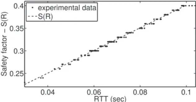
Figure 4: Safety factor vs round trip time.

length, and the frame rate. In particular, and based on the debug information provided by the Akamai Client and on the experiments we have run, the stream-switching heuris-tic works as follows.

The client periodically issues rtt-test commands that have the effect of setting at the server a throttling percent-age of 500%, thus asking the server to periodically send the video in greedy mode. In this way Akamai actively probes for extra available bandwidth and estimates the RTTR(t) under congestion. Based on the estimated value of the RTT, the client computes asafety factorS. By parsing the debug information in order to collect the pairs (R(t), S(t)) shown in Figure 4, it was possible to run a linear regression over the dataset which yielded to the following static linear model (R(t) is expressed in seconds):

f(R(t)) = 2.5R(t) + 0.15

We have observed that whenR(t) >0.1s the safety factor remains set to 0.4, whereas whenR(t) <0.02s, it is set to 0.2. Thus, we can conclude that the complete model for

S(R(t)) is the following: S(R(t)) =      0.2 0< R(t)<0.02s 2.5R(t) + 0.15 0.02s≤R(t)≤0.1s 0.4 R(t)>0.1s (3)

For each video level li ∈ L a high threshold LHi and a

low thresholdLL

i are maintained:

LHi (t) =li·(1 +S(t)) ; LLi =li·1.2 (4)

A switch up (SWITCH UP) to a higher video levelliis enabled

only if B(t) > LH

i (t), which means that if, for instance,

the RTT is above 0.1 s and thus S(R(t)) = 0.4, in order to switch to level li the estimated bandwidth must be at

least 40% higher thanli. This seems to be a conservative

approach that leads to network underutilization and, as a consequnece, to a reduced QoE.

The switch down event occurs when:

q(t)< qL(t) (5)

where qL(t) is another threshold that is smaller than the

queue target3 qT(t). When (5) holds, aBUFFER FAILUREis

sent and the new video levelli< l(t) is selected. In

partic-ular, the highest video levelli∈L satisfying the following

condition:

B(t)>1.2·li=LLi 3

The identification ofqL(t) has not been carried out.

Internet Levels Video buffer li∈L q(t) l(t) selects Controller Server sender traffic HTTP r(t), l(t) Decoder buffer Player τf

Figure 5: QAC control architecture

is selected. Thus, in to select the level li, the currently

estimated bandwidth B(t) must be at least 20% above li.

Moreover, in [5] we have shown that when SWITCH UP and

BUFFER FAILURE commands are sent from the client, the

actuator, which is located at the server, takes a delay of

τsu '14s andτsd'7s respectively, to actuate these

com-mands.

Finally, it is worth noting that the overall system ex-hibits a very complex dynamics due to the interaction of two closed-loop dynamics: the stream-switching logic, which has been designed using heuristic arguments, and the buffer level controller. As a consequnce, it is very complex to develop a mathematical analysis as well as to tune control variables to satisfy key design requirements such as settling times and steady state errors.

4. QUALITY ADAPTATION CONTROLLER

In this Section we propose aQuality Adaptation Controller

(QAC) for adaptive live video streaming that aims at pursu-ing the followpursu-ing goals: 1)maximize the QoE by delivering the best quality that is possible given the network avail-able bandwidth while minimizing playback interruptions; 2)

rigorous design of the controller by employing the control theory; 3) high scalability in terms of processing costs; 4)

CDN-friendly design, i.e. the algorithm can be easily de-ployed on CDNs; 5)codec-agnostic,i.e. the service provider has the freedom to choose any codec.

In order to pursue the goals 3), 4), and 5) we choose thestream-switchingapproach and we employ the standard HTTP streaming over TCP. For what concerns the goals 1) and 2) we employ feedback control theory to design a con-troller that throttles the video levell(t) to be streamed with-out using any heuristics. This provides the key advantage of getting a predictable system dynamics that can fulfill re-quired design features such as settling time and steady state errors [6].

4.1 The control system

Figure 5 shows the architecture of the proposed streaming server. The first important differencewrt the control archi-tecture employed by Akamai (Figure 3) is that measuring, control and actuation take place at the server so that the control loop is not affected by delays and does not require explicit feedback from the client. This architecture provides the following advantages: 1)simplicity of the player: being the control centralized at the server, the player at the client has the only task of decoding and playing the stream; more-over, when a new version of the control algorithm is designed and installed at the server, there is no need to update the

(6)

1 s sender buffer − q(t) qT(t) l(t) − u(t) Controller Quantizer Gc(s) b(t)

Figure 6: Block diagram of the control loop

player; 2)effectiveness of the controller: by avoiding delays in the control loop the controller can provide faster dynam-ics while retaining stability [6].

The controller works as follows: it takes as input the queue lengthq(t) of thesender buffer that is placed at the server, and it selects the video levelli∈L. The selected video level

is temporally stored at the sender buffer and is then sent to the client via a TCP connection. The received stream is buffered at the client that decodes and plays the video content.

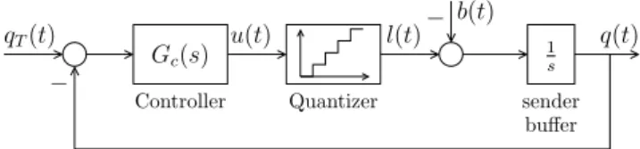
Figure 6 shows a block diagram of the feedback control system designed to throttle the video levell(t). In the follow-ings∈Cdenotes the Laplace variable andF(s) =L {f(t)}

denotes the unilateral Laplace transform of the real valued functionf(t).

The input of the systemqT is the set-point, or threshold

value, for the sender buffer lengthq(t).The controller goal is to track a queue lengthqT >0 so that the TCP sender

buffer is always full and can fill the communication pipe. The controller, which can be described by its transfer function Gc(s), takes as input the error e(t) = qT −q(t)

and outputs the control signalu(t) that is the bitrate the encoder should set to match the available bandwidthb(t). In our case, since we employ the stream-switching approach, the video bitrate will belong to the discrete set of available video levelsL. This can be modelled through a quantizer, which is a static element that takes as inputu(t) and se-lects the highest video levellithat is less thenu(t). Finally,

the sender buffer, which can be modelled by the integrator 1/s, is filled at a ratel(t) and it is drained by the available bandwidth at the rateb(t). It is worth to notice that the available bandwidthb(t) is modelled as a disturbance [13].

The effect of the quantizer is to add a quantization error

dq(t) = l(t)−u(t) tou(t). This is equivalent to consider

dq(t) as a disturbance acting onb(t) giving the total

equiv-alent disturbancedeq(t) =b(t) +dq(t). In this way we are

able to take the quantizer out of the control loop and we can compute the transfer function from the inputqT to the

outputq(t) as follows: G0(s) = Q(s) QT(s) = Gc(s) 1 s 1 +Gc(s)1_s (6)

We choose a proportional integral (PI) controller:

Gc(s) =

U(s)

E(s) =Kp+

Ki

s (7)

since it is able to reject step-like disturbances b(t) and it is very simple to be discretized and implemented in a soft-ware module. The integral action of the controller ensures that the video level l(t) matches on average the available bandwidthb(t). E M U D X E R O P G O P G O P G Video input Client Internet l1 l2 lN Module Encoder Video levels storage Producer Module l_i(k) q(t) i(k) QAC

Figure 7: The QAC adaptive streaming server ar-chitecture

By substituting (7) in (6) it turns out:

G0(s) =

Kps+Ki

s2₊_K ps+Ki

(8)

Thus, the closed loop system is a second order system with one zero. In order to tune the controller, we impose the damping factor of the system (8) to beδ=√2/2 [6] and a natural frequencyωn=

√

Ki= 0.1886 rad_s that corresponds

to a system bandwidth of around 0.06 Hz and a 2% settling time of Ts = _δω4

n = 30 s. This choice is made in order to

limit the switching frequency between different video levels. The gains of the PI turn out to beKi= 0.0356 andKp=

0.2667.

In the time domain the control law is:

u(t) =L−1{Gc(s)E(s)}=Kpe(t) +Ki

ˆ t

0

e(ξ)dξ (9)

In order to implement (9) we need to discretize the control law with a sampling time ∆T:

u(tk) =Kpe(tk) +Ki k X

j=0

∆T e(tj) (10)

We choose a sampling time ∆T = 0.5s that is 1/60th of the settling timeTs. In the following subsection we provide

the implementation details of the adaptive streaming server using the QAC.

4.2 Implementation of the adaptive streaming

server

The adaptive streaming server is written in Python and developed using the Twisted4 _{libraries. A schematic}

rep-resentation of the proposed streaming server is shown in Figure 7. The server contains an audio/video transcod-ing engine (Encoder Module) developed ustranscod-ing GStreamer5

and FFMpeg6 libraries. The encoder module takes as in-put a raw or pre-encoded audio/video file and outin-puts a set of files transcoded at various bitrates and resolutions. We used the same levels of AHDVS as shown in Table 1 with a frame rate equal to 30 fps. We employ a fixed Group of Picture (GOP) of 30 frames which is equal to 1s of video stream. For each transcoded file, the encoder module stores an index file (.index) containing the file position and the timestamp of each encoded GOP. We used a fixed GOP

4

http://twistedmatrix.com/ 5_{http://gstreamer.org/} 6

(7)

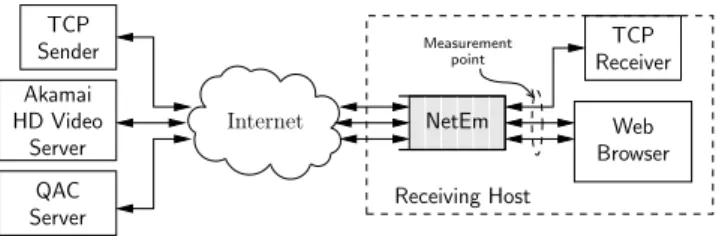
Akamai HD Video Server Receiver TCP Sender TCP Internet QAC Server Web Browser Measurement point Receiving Host NetEm

Figure 8: Testbed employed in the experimental

evaluation

encoder setting in order to simplify the stream switch be-tween video levels. Moreover, the server integrates also a Producer Module, which is a simple HTTP server. When a client connects to the server, it sends a GET HTTP re-quest specifying the stream unique identifier it wants to play. The producer replies with a HTTP response and starts to send the video stream content reading from the storage at a configured start level7l(0) = ¯l. Moreover, the producer con-tinuously provides the current queue levelq(t) to the QAC module. When a video level switch occurs, the producer selects the corresponding input file from the storage, it per-forms a file seek operation to the current sent time position using the information contained in the.indexfile and then it feeds the data to the client. The switch operation can be performed only at GOP boundaries in order to ensure the correct decoding by the client.

The adaptive streaming server supports every encoding format provided by GStreamer/FFMpeg libraries. In this paper, in order to make a fair comparison with AHDVS, we encoded the video using H.264 codec and MP3 audio muxed into FLV container.

It is worth noticing that the producer and the QAC mod-ules are independent from the encoding profile used. Finally, we stress that the client can be not only an Adobe Flash ap-plet, but also any video player that supports the same codec employed by the server. A buffering time of 15s at the client side is recommended in order to avoid interruptions.

5. EXPERIMENTAL EVALUATION

In this section we carry out a comparison between the Akamai HD video server and the proposed Quality Adapta-tion Controller (QAC) by employing the testbed shown in Figure 8. To run the experiments, we have employed the video sequence “Elephant’s Dream”8 _{since its duration is}

long enough for a careful experimental evaluation. In order to perform a fair comparison, the video sequence streamed with the QAC has been encoded using the x264 codec and the same discrete set of video levels employed by AHDVS (see Table 1). The receiving host is an Ubuntu Linux ma-chine running 2.6.32 kernel equipped with NetEm, which is a kernel module that, along with the traffic control tools avail-able on Linux kernel, allows downlink channel bandwidth and delays to be set. In order to perform traffic shaping on the downlink we have used the Intermediate Functional Block pseudo-device IFB9.

The receiving host was connected to the Internet through our campus wired connection. It is worth to notice that,

7

In this paper we used a start video levell(0) =l1

8_{http://orange.blender.org/} 9

http://linuxfoundation.org/collaborate/workgroups/networking/ifb

before running any experiment, we carefully checked that the available bandwidth was well above 4 Mbps, which is the maximum value of the bandwidth we set in the traffic shaper. The measured RTT between our client and the Aka-mai server was in the range 10ms to 30ms. All measurements have been taken after the traffic shaper (as shown in Figure 8) and collected by sniffing the traffic on the receiving host

with tcpdump. For what concerns AHDVS, the dump files

have been post-processed and parsed using a Python script to obtain the figures that we report in the following.

The receiving host runs aniperfserver (TCP Receiver) in order to receive TCP greedy flows sent by aniperfclient (TCP Sender).

Four different scenarios have been considered in order to investigate the dynamic behaviour of the two considered quality adaptation algorithms: 1) one video stream over a bottleneck link whose available bandwidth changes following a step function with minimum value of 500 kbps and max-imum value of 4000 kbps; 2) one video stream over a bot-tleneck link whose available bandwidth varies as a square wave with a period of 200s, a minimum value of 500 kbps and a maximum value of 4000 kbps; 3) one video stream sharing a bottleneck, whose available bandwidth is equal to 4000 kbps, with one concurrent TCP flow; 4) two video streams sharing a bottleneck whose available bandwidth is equal to 4000 kbps.

In scenarios 1 and 2 abrupt variations of the available bandwidth occur: such step-like variations of the input sig-nal are often employed in control theory to evaluate key features of a dynamic system response to an external input such as settling time, overshoots and time constants [4]. The third scenario evaluates the dynamic behaviour of a video flow when it shares the bottleneck with a greedy TCP flow, such as in the case of a file download, and it is useful to investigate the inter-protocol fairness.

Since, due to the use of TCP, the loss rate is small, the evaluation of the QoE can be inferred by evaluating the in-stantaneous video level received by the client, i.e., the higher the received video levell(t) the higher the quality perceived by the user. For this reason we employ the received video level l(t) as the key performance index of the system. In particular, to assess the efficiency of the quality adaptation algorithm, we introduce the following index of utilization:

η= ˆl

C (11)

where ˆl is the average value of the video level l(t), C = min(lM, b) where lM is the maximum video level and b is

the available bandwidth. The index 0 ≤ η ≤1 is 1 when the average value of the received video level is equal toC, i.e. when the video level exactly matches the bottleneck available bandwidth.

For each considered scenario we will show the dynamics of the following variables: the received video levell(t), the received video rate r(t), the decoded frame rate f(t), and the receiver buffer lengthq(t).

5.1 Step-like change of the bottleneck capacity

We start by investigating the dynamic behaviour of the two quality adaptation algorithms in a simple scenario. The bottleneck available bandwidth b(t) increases at time t = 50s from a value of Am = 500 kbps to a value of AM =

(8)

0 50 100 150 200 250 300 L0=300 L1=700 1000 L2=1500 2000 L3=2500 3000 L4=3500 4000 4500 5000 time (sec) kbps l(t)

Received video rate b(t)

(a) Received rater(t), video levell(t), and available bandwidth

b(t) 0 50 100 150 200 250 300 0 10 20 30 time (sec)

Receiver queue (sec)

(b) Receiver buffer length

0 50 100 150 200 250 300 0 10 20 30 time (sec) frame rate (fps) (c) Frame ratef(t)

Figure 9: QAC adaptive video streaming response to a step change of available bandwidth att= 50s

In particular, we are interested in assessing the responsive-ness of the adaptation algorithms in matching the available bandwidth choosing the adequate video level l(t). Figure 9 and Figure 10 show the dynamics of one QAC and one AHDVS video flow, respectively.

Let us consider Figure 9(a) that shows the received video rater(t) and video levell(t) in the case of QAC: after that the bandwidth increases att= 50s, the video level increases and eventually reaches, at steady state, the maximum video level l4 after a transient time of around 30s. It is worth

noting that the transient time required for l(t) to match the available bandwidth b(t) is equal to the settling time

Ts that was set as requirement when the quality controller

was designed (7) (see Section 4). Moreover, Figure 9(b) shows that the received buffer length is 15s throughout all the duration of the connection. The decoded frame rate of the stream oscillates around 30 fps, which proves that there were no video interruptions during the streaming. Finally, the efficiency index (11) is 0.93.

Let us now focus on the Akamai video streaming server. Figure 10(a) shows the dynamics of the video levell(t), the estimated bandwidth reported by thelvl1 parameter, and

0 50 100 150 200 250 300 L0=300 L1=700 1000 L2=1500 2000 L3=2500 3000 L4=3500 4000 4500 5000 time (sec) kbps b(t) Estimated BW l(t) BF SU r(t)

(a) Estimated BW, video level l(t), received rate r(t),

BUFFER FAILURE, andSWITCH UPevents

0 50 100 150 200 250 300 0 5 10 15 20 25 sec time (sec)

Buffer Buffer target

(b) Receiver buffer length and target buffer length

0 50 100 150 200 250 300 0 10 20 30 time (sec) Frame rate (fps) (c) Frame ratef(t)

Figure 10: AHDVS response to a step change of available bandwidth at t= 50s

the received video rater(t). In order to show their effect on the dynamics ofl(t), Figure 10(a) also reports the time in-stants at whichBUFFER FAILURE (BF) andSWITCH UP(SU) commands are issued. The video level is initialized at l0

that is the lowest available version of the video. Neverthe-less, at timet= 0 the estimated bandwidth is erroneously overestimated to a value above 3000 kbps and a SWITCH UP

command is sent to the server. The effect of this command occurs after an actuation delay ofτsu = 7.16s (see Section

3) when l(t) is increased to l3 = 2500 kbps, which is the

video level closest to the bandwidth estimated at t = 0. By setting the video level tol3, which is above the current

available bandwidth Am = 500 kbps, the receiver buffer

starts to drain and it eventually gets empty at t = 17.5s (see Figure 10(b)). Figure 10(c) shows that during the time interval [17.5,20.8]s the playback frame rate is zero, meaning that the video is paused. At time t = 18.32s, a

BUFFER FAILURE command is finally sent to the server.

Af-ter a delay of aboutτsd= 16s the server switches the video

level tol0= 300 kbps that is below the available bandwidth

Am. Even though the heuristic to trigger a video level switch

down (5) should be able in principle to avoid interruptions, the actuation delayτsdposes a remarkable limitation to the

(9)

responsiveness of the quality adaptation algorithm. More-over, Figure 10(a) shows that the transient time required byl(t) to reach the maximum video levell4 is around 150s,

which is roughly one order of magnitude higher than the transient time exhibited by QAC. Finally, in this case the efficiency index (11) is 0.676 that is well below the value found in the case of QAC. To conclude, the inefficiency of AHDVS is largely due to the conservativeness of the safety-factorS(t) that we discussed in Section 3. In fact, given a minimum safety factor ofS= 0.2, the available bandwidth required to switch to the levell4 = 3500 kbps according to

(4) turns out to be 4200 kbps that is aboveAM.

Let us compare the received video rates of QAC and AHDVS shown respectively in Figure 9(a) and 10(a): if on one hand the received video rate of QAC is affected by a moderate burstiness that is typical of a TCP connection, on the other hand the received rate of AHDVS is affected by remarkable and persistent oscillations whose amplitude is more than 2Mbps. This is due to the fact that AHDVS dynamics pe-riodically switches between two states: in thenormal state the video sending rate is bounded by the maximum sending rater(t) given by (2), whereas each time artt-test com-mand is issued AHDVS enters thegreedy-modestate and for a short time interval of around 5s the sending rate is limited by the available bandwidth [5].

In conclusion, this experiment shows that QAC is able to provide the maximum value of the received video level that is possible given the available bandwidth with a tran-sient time of around 30s in accordance with the design re-quirements given in Section 4. On the other hand, AHDVS exhibits a very large transient of around 150s, remarkable oscillations in the received rater(t), it is not able to provide the maximum possible QoE to the user, and it is not able to avoid interruptions.

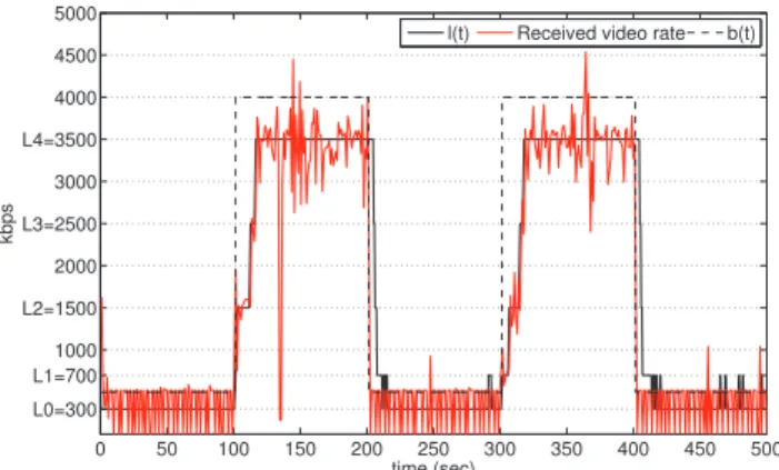
5.2 Square-wave varying bottleneck capacity

In this experiment we consider abrupt drops/increases of the bottleneck available bandwidth b(t) which is shaped as a square-wave function with a period of 200s, a mini-mum value Am = 500 kbps and a maximum valueAM =

4000 kbps. The aim of this experiment is to assess the re-sponsiveness of the two considered adaptive video stream-ing services in shrinkstream-ing the video levell(t) in response to an abrupt drop of the available bandwidth and to what ex-tent they are able to guarantee a continuous reproduction of the video content in the presence of this sudden bandwidth reduction.

Figure 11(a) shows the dynamics of the video received rate r(t) and the video level l(t) in response to the avail-able bandwidth b(t). The figure shows that the QAC al-gorithm is able to control l(t) so that it properly follows step increases and decreases in the available bandwidth. In particular, the transient times required for l(t) to match bandwidth increases/decreases are less than 20s. Moreover, Figures 11(b) and 11(c) show that the receiver buffer length is around 15s and the reproduced frame rate is around 30 fps during all the experiment, so showing a reproduction with-out interruptions. During the time intervals with bandwidth

AM = 4000 kbps, the efficiency index was equal to 0.93.

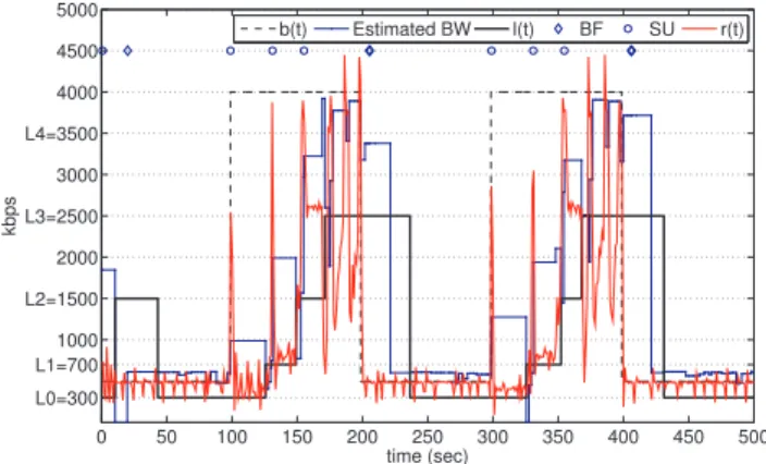
On the other hand, Figure 10 clearly shows that AHDVS is not able to properly adapt the video level to follow band-width variations. By considering the dynamics of the video levell(t) shown in Figure 12(a) we notice two main facts:

0 50 100 150 200 250 300 350 400 450 500 L0=300 L1=700 1000 L2=1500 2000 L3=2500 3000 L4=3500 4000 4500 5000 time (sec) kbps

l(t) Received video rate b(t)

b(t) 0 50 100 150 200 250 300 350 400 450 500 0 10 20 30 time (sec)

(b) Receiver buffer length

0 50 100 150 200 250 300 350 400 450 500 0 10 20 30 time (sec) frame rate (fps) (c) Frame ratef(t)

Figure 11: QAC response to a square-wave available bandwidth with period 200s

1) when the available bandwidth increases toAM the video

level is increased tol3, which is less than the maximum video

levell4, in around 75s; 2) when bandwidth drops occur the

playback is affected by interruptions as it can be inferred by considering Figure 12(b) and Figure 12(c). In partic-ular, when the first bandwidth drop occurs at t= 200s, a

BUFFER FAILURE is sent to the server after a delay of roughly

7s in order to switch down the video level froml3tol0. After

that, a switch-down delay τsd of 20s occurs and the video

levell(t) is finally switched tol0. Thus, the total delay spent

to correctly set the video levell(t) to match the new value of the available bandwidth is 38s. Due to this large delay in settingl(t), the receiver buffer gets empty and the reproduc-tion of the video is blocked for more than 100s. The same situation occurs when the second bandwidth drop occurs. In this case, the total delay spent to correctly set the video level is 26s. Again, 13s after the second bandwidth drop, an interruption in the video reproduction occurs. During the time intervals with bandwidthAM = 4000 kbps, we

evalu-ated a low index of efficiency equal to 0.4, which is less than half the efficiency obtained by QAC in this scenario.

(10)

pro-0 50 100 150 200 250 300 350 400 450 500 L0=300 L1=700 1000 L2=1500 2000 L3=2500 3000 L4=3500 4000 4500 5000 time (sec) kbps b(t) Estimated BW l(t) BF SU r(t)

0 50 100 150 200 250 300 350 400 450 500 0 10 20 sec time (sec)

(b) Receiver buffer length and target buffer length

0 50 100 150 200 250 300 350 400 450 500 0 10 20 30 time (sec) Frame rate (fps) (c) Frame ratef(t)

Figure 12: AHDVS response to a square-wave avail-able bandwidth with period200s

posed QAC is able to control l(t) to follow step increases and decreases of the available bandwidth always providing the user with a continuous reproduction of the video content at the best QoE. In the case of Akamai HD Video Streaming, when the available bandwidth suddenly shrinks, the video reproduction is affected by interruptions.

5.3 One concurrent greedy TCP flow

In this experiment we investigate the performance of the two quality adaptation algorithms when sharing the avail-able bandwidth with one greedy TCP flow, such as in the case of a parallel download session. The available band-width has been set to a constant value of 4000 kbps, a video streaming session is started att= 0, a greedy TCP connec-tion is started att= 150s and it is stopped att= 360s.

Figure 13(a) shows the dynamics of the video levell(t) and of the video received rater(t), whereas Figure 13(b) shows the goodput of the concurrent TCP flow. In the first part of the experiment, for 0< t < 150s,l(t) quickly matches the available bandwidth obtaining an efficiencyη= 0.98. After the greedy TCP flow is started att= 150s the video level

l(t) is switched down in about 10s and, since the fair share is

0 50 100 150 200 250 300 350 400 450 500 L0=300 L1=700 1000 L2=1500 2000 L3=2500 3000 L4=3500 4000 4500 5000 time (sec) kbps

l(t) Received video rate b(t)

b(t) 0 50 100 150 200 250 300 350 400 450 500 L0=300 L1=7001000 L2=15002000 L3=2500 3000 L4=35004000 4500 5000 time (sec) (kbps) TCP goodput Fair share Average TCP goodput (b) TCP goodput 0 50 100 150 200 250 300 350 400 450 500 0 10 20 30 time (sec)

(c) Receiver buffer length

Figure 13: QAC when sharing the bottleneck with one greedy TCP flow

2000 kbps,l(t) switches between the two closest video levels

l2 = 1500 kbps and l3 = 2500 kbps. In this part of the

experiment the efficiency is 0.99 and, the average goodput of the greedy TCP flow is 1930 kbps whereas the goodput obtained by QAC flow is 1910 kbps thus indicating that the two flows share the available bandwidth fairly. When the greedy TCP flow is stopped, the video levell(t) is correctly set to the maximum video level l4 after a transient of 4s.

In this part of the experiment the efficiency of QAC is 0.99. Finally, Figure 13(c) shows that the receiver buffer length is always greater than 15s, meaning that no interruptions occurred during the video reproduction.

Figure 14(a) shows the video level dynamicsl(t), the es-timated bandwidth and the received video rate r(t) in the case of AHDVS. During the first part of the experiment, i.e. fort <150s, apart from a short time interval [6.18,21.93]s during whichl(t) is equal tol4= 3500 kbps, the video level

is set tol3= 2500 kbps. The efficiency indexηin this part of

the experiment is 0.74. When the TCP flow joins the bottle-neck, it grabs the fair bandwidth share of 2000 kbps. Nev-ertheless, the estimated bandwidth decreases to the correct value after 9s. After an additional delay of 8s, at t= 167s,

(11)

0 50 100 150 200 250 300 350 400 450 500 L0=300 L1=700 1000 L2=1500 2000 L3=2500 3000 L4=3500 4000 4500 5000 time (sec) kbps b(t) Estimated BW l(t) BF SU r(t)

0 50 100 150 200 250 300 350 400 450 500 L0=300 L1=700 L2=15002000 L3=2500 3000 L4=35004000 4500 5000 time (sec) kbps

TCP goodput Fair Share Average TCP goodput

(b) TCP goodput 0 50 100 150 200 250 300 350 400 450 500 0 5 10 15 20 25 sec time (sec)

(c) Receiver buffer length and target buffer length

Figure 14: AHDVS when sharing the bottleneck

with one greedy TCP flow

video level is shrunk to the suitable valuel2 = 1500 kbps

after a total delay of 24s. In this case, this actuation delay does not affect the video reproduction as it can be inferred by considering the receiver buffer dynamics shown in Fig-ure 14(c). However, FigFig-ure 14(a) shows thatl(t) is further decreased to l1 = 700 kbps and it is set to steady state

value ofl2 at t= 212s. Thus, the transient time spent to

reach the steady state is 62s. In this part of the experiment, the efficiency index is equal to 0.76, the average goodput of the greedy TCP flow is 2170 kbps, whereas the goodput obtained by Akamai flow is 1643 kbps indicating that the available bandwidth is underutilized. In the third part of the experiment, after the TCP flow leaves the bottleneck at timet = 360s, the level is switched up tol3 = 2500 kbps

with a delay of 26s. In this part of the experiment the effi-ciency is 0.69. Finally, by considering Figure 14(b), we can observe that the “on-off” dynamics of the sending rate pro-vided by AHDVS affects the dynamics of the TCP received rate that shows remarkable oscillations.

5.4 Two concurrent video streaming sessions

In this scenario we evaluate the behaviour of two video streams that share the same bottleneck whose available

band-0 50 100 150 200 250 300 350 400 450 500 L0=300 L1=7001000 L2=1500 2000 L3=2500 3000 L4=3500 4000 4500 5000 time (sec) kbps l 1(t) l 2(t) b(t)

(a) Received video levelsl1(t),l2(t)

0 50 100 150 200 250 300 350 400 450 500 L0=300 L1=7001000 L2=1500 2000 L3=2500 3000 L4=3500 4000 4500 5000 time (sec) kbps r 1(t) r 2(t) b(t)

(b) Received ratesr1(t) andr2(t)

0 50 100 150 200 250 300 350 400 450 500 0 5 10 15 20 25 30 time (sec)

receiver queue 1 receiver queue 2

(c) Receiver queue of the two concurrent video flows

Figure 15: Two QAC adaptive video streaming flows sharing a bottleneck

width has been set to 4000 kbps. The first video streaming session is started att= 0 and after 100s a second video flow is started. This experiment is aimed at assessing to what extent two competing flows are able to share in a fair way the bottleneck. In this experiment the fair share is equal to 2000 kbps.

Figure 15(a) shows the dynamics of the video levelsl1(t)

and l2(t) of the first and the second video flow controlled

by QAC. In the first part of the experiment, the first flow behaves as already shown in the other experiments quickly settingl1(t) to the maximum video levell4. When the

sec-ond video flow joins the bottleneck at t= 100s, the video level l1(t) is correctly shrunk to let the second video flow

obtain its fair share. After a transient time of 8s the two video levels l1(t) andl2(t) start to switch between the two

video levels, l2 = 1500 kbps and l3 = 2500 kbps, that are

closest to the fair share which is 2000 kbps.

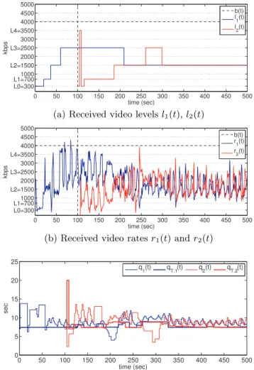
Figure 16(a) shows the dynamics of the two video levels in the case of AHDVS. The figure shows that, when the second flow joins the bottleneck, it takes 210s for the video level l1(t) to be set to the correct value l2 = 1500 kbps.

Thus, during this transient the first video flow experiences a higher video level with respect to the second video flow,

(12)

0 50 100 150 200 250 300 350 400 450 500 L0=300 L1=7001000 L2=1500 2000 L3=2500 3000 L4=3500 4000 4500 5000 time (sec) kbps b(t) l 1(t) l 2(t)

(a) Received video levelsl1(t),l2(t)

0 50 100 150 200 250 300 350 400 450 500 L0=300 L1=7001000 L2=1500 2000 L3=2500 3000 L4=3500 4000 4500 5000 time (sec) kbps b(t) r 1(t) r 2(t)

(b) Received video ratesr1(t) andr2(t)

0 50 100 150 200 250 300 350 400 450 500 0 5 10 15 20 25 sec time (sec) q₁(t) q_T,1(t) q₂(t) q_T,2(t)

(c) Receiver buffer lengths q1(t) andq2(t) and target buffer

lengthsqT ,1(t),qT ,2(t)

Figure 16: Two AHDVS flows sharing a bottleneck

indicating that the controller is not able to provide the same QoE to all the users sharing a bottleneck.

Finally, Table 3 collects the average goodputs g1 and g2

obtained for t > 100s by the first and the second flow re-spectively for both QAC and AHDVS streaming systems. The average channel utilization, computed as U = (g1 +

g2)/4000 kbps, obtained by QAC results 10% higerwrtthe

one obtained by AHDVS.

6. CONCLUSIONS

In this paper we have presented a Quality Adaptation Controller (QAC) for a stream-switching adaptive live video streaming system designed by using feedback control theory. Moreover, we have provided a characterization of the adap-tation algorithm employed by Akamai High Definition Video Server which also implements a stream-switching system.

The main results of the paper are the following: 1) QAC is able to control the video levell(t) to match the available bandwidthb(t) with a transient time that is less than 30s always providing a continuous video reproduction; 2) the proposed controller is able to share in a fair way the avail-able bandwidth both in the case of a concurrent greedy con-nection and a concurrent video streaming flow; 3) Akamai underutilizes the available bandwidth due to the

conserva-Server g1 g2 U

QAC 1860 1950 0.95 AHDVS 1815 1612 0.85

Table 3: Goodput g1 and g2 (kbps) of the two con-current flows and channel utilizationU

tiveness of its algorithm based on heuristics; 4) moreover, when abrupt reductions of the available bandwidth occur, the video reproduction is affected by interruptions.

7. REFERENCES

[1] Akamai HD Network Demo.

http://wwwns.akamai.com/hdnetwork/demo/flash. [2] Move Networks HD adaptive video streaming.

http://www.movenetworkshd.com.

[3] Adobe Systems Inc. Real-Time Messaging Protocol (RTMP) Specification. 2009.

[4] L. De Cicco and S. Mascolo. A Mathematical Model of the Skype VoIP Congestion Control Algorithm.IEEE Trans. on Automatic Control, 55(3):790–795, Mar. 2010.

[5] L. De Cicco and S. Mascolo. An Experimental Investigation of the Akamai Adaptive Video Streaming. InProc. of USAB 2010, Nov. 4–5, 2010. [6] G. Franklin, J. Powell, and A. Emami-Naeini.Feedback

control of dynamic systems. Addison-Wesley, 1994. [7] M. Handley, S. Floyd, and J. Pahdye. TCP Friendly

Rate Control (TFRC): Protocol Specification.RFC 3448, Proposed Standard, Jan. 2003.

[8] D. Hassoun. Dynamic streaming in flash media server 3.5. Available:

http://www.adobe.com/devnet/flashmediaserver/. [9] C. Krasic, J. Walpole, and W. Feng. Quality-adaptive

media streaming by priority drop. InProc. of ACM NOSSDAV ’03, 2003.

[10] R. Kuschnig, I. Kofler, and H. Hellwagner. An evaluation of TCP-based rate-control algorithms for adaptive internet streaming of H. 264/SVC. InProc. of ACM SIGMM conference on Multimedia systems, pages 157–168, 2010.

[11] R. Pantos and W. May. HTTP Live Streaming.IETF Draft, June 2010.

[12] M. Prangl, I. Kofler, and H. Hellwagner. Towards QoS Improvements of TCP-Based Media Delivery. InProc. of ICNS ’08, pages 188–193, 2008.

[13] S. Mascolo. Congestion control in high-speed communication networks using the Smith principle.

Automatica, 35(12):1921–1935, 1999.

[14] H. Schulzrinne, A. Rao, and R. Lanphier. Real Time Streaming Protocol (RTSP).RFC 2326, Standard track, Apr. 1998.

[15] V. Jacobson. Congestion avoidance and control. In

Proc. of ACM SIGCOMM ’88, pages 314–329, 1988. [16] B. Wang, J. Kurose, P. Shenoy, and D. Towsley.

Multimedia streaming via TCP: An analytic performance study. ACM TOMCCAP, 4(2):1–22, 2008.

[17] A. Zambelli. IIS smooth streaming technical overview.

Feedback Control for Adaptive Live Video Streaming