4.7. Canonical ordination

4.7. Canonical ordination

4.7.1 Introduction

The ordination methods reviewed above are meant to represent the variation of a data matrix in a reduced number of dimensions. Interpretation of the structures is done a posteriori, hence the expression indirect (gradient) analysis used for this approach. For instance, one can interpret the CA ordination axes (one at a time), by regressing the object scores on one or several environmental variables. The ordination procedure itself has not been influenced by these external variables, which become involved only after the computation. One lets the data matrix express itself without constraint. This is an exploratory, descriptive approach.

Constrained ordination [redundancy analysis (RDA) and canonical correspondence analysis (CCA)], on the contrary, explicitly puts into relationship two matrices: one response matrix and one explanatory matrix. Both are involved at the stage of the ordination. This approach

integrates the techniques of ordination and multiple regression

(Table VIII):

Table VIII - Relationship between ordination and regression

Response variables Explanatory variables Analysis

1 variable 1 variable Simple regression

1 variable m variables Multiple regression

p variables - Simple ordination

p variables m variables Canonical ordination

In RDA and CCA, the ordination process is directly influenced by a set of explanatory variables: the ordination computes axes that are a

linear combination of explanatory variables. In other words, these

explain the variation of the response matrix. It is therefore a

constrained ordination process. The difference with an unconstrained ordination is important: the matrix of explanatory variables conditions the "weight" (eigenvalues), the orthogonality and the direction of the ordination axes. Here one can say that the axes

explain (in the statistical sense) the variation of the dependent matrix.

A constrained ordination produces as many canonical axes as there are explanatory variables, but each of these axes is a linear combination (a multiple regression model) of all explanatory variables. Examination of the canonical coefficients (i.e., the regression coefficients of the models) of the explanatory variables on each axis allows to know which variable(s) is or are most important to explain the first, second... axis.

The variation of the data matrix that cannot be explained by the environmental variables is expressed on a series of unconstrained axes following the canonical ones.

Due to the fact that in many cases the explanatory variables are not dimensionally homogeneous, usually canonical ordinations are done with standardized explanatory variables. In RDA, this does not affect the choice between running the analysis on a covariance or a correlation matrix, however, since this latter choice relates to the response (y) variables.

4.7.2 Renduncandy analysis (RDA)

Depending on the algorithm used, the search for the optimal linear combinations of explanatory variables that represent the orthogonal canonical axes is done sequentially (axis by axis, using an iterative algorithm) or in one step (direct algorithm). Figure 26, which is Figure 11.2 of Legendre & Legendre (1998, p. 581), summarises the steps of a redundancy analysis (RDA) using the direct algorithm:

- regress the p response variables, each one separately, on the explanatory variables; compute the fitted and residual values of the regressions;

- run a PCA of the matrix of fitted values of these regressions;

- use the matrix of canonical eigenvectors to compute two sorts of site ordinations:

- an ordination in the space of the explanatory variables; this yields the fitted site scores, called "Site constraints (linear combinations of constraining variables)" in the vegan library of R; these canonical axes are orthogonal to one another;

- an ordination in the space of the response variables (species space); this yields the "sample scores" of Canoco; in vegan, these site scores are called "Site scores (weighted sums of species scores)". These ordination axes are not orthogonal;

- use the matrix of residuals from the multiple regressions to compute an unconstrained ordination (PCA in the case of an RDA).

Redundancy analysis (RDA) is the canonical counterpart of principal component analysis (PCA). Canonical correspondence analysis (CCA) is the canonical counterpart of correspondence analysis (CA).

Due to various technical constraints, the maximum numbers of canonical and non-canonical axes differ (Table IX):

Table IX - Maximum number of non-zero eigenvalues and corresponding eigenvectors that

may be obtained from canonical analysis of a matrix of response variables Y(n×p) and a

matrix of explanatory variables X(n×m) using redundancy analysis (RDA) or canonical

correspondence analysis (CCA). This is Table 11.1 from Legendre & Legendre (1998, p.588).

Canonical eigenvalues Non-canonical eigenvalues

and eigenvectors and eigenvectors

RDA min[p, m, n–1] min[p, n–1]

Regress each variable y on table X and

compute the fitted (y) and residual (y^ _res) values

Data table

Y

X

multiple regressions PCA

Y = X [X'X] X'Y^ –1 U = matrix of eigenvectors (canonical) YU = ordination in the space of variables X ^ YU = ordination in the space of variables Y Residual values from the

multiple regressions PCA

Y_res = Y – Y^ U_res = matrix of eigenvectors (of residuals) Y_resU_res = ordination in the space of residuals

Figure 26 - (preceding page) The steps of redundancy analysis using a direct algorithm.

This is Figure 11.2 of Legendre & Legendre (1998).

Graphically, the results of RDA and CCA are presented in the form of

biplots or triplots, i.e. scattergrams showing the objects, response

variables (often species) and explanatory variables on the same diagram. The explanatory variables can be qualitative (the multiclass ones are declared as "factor" in vegan but must be coded as a series of dummy binary variables in Canoco) or quantitative. A qualitative explanatory variable is represented on the bi- or triplot as the centroid of the sites that have the description "1" for that variable ("Centroids for factor constraints" in vegan, "Centroids of environmental variables" in Canoco), and the quantitative ones are represented as vectors (the vector apices are given under the name "Biplot scores for constraining variables" in vegan and "Biplot scores of environmental variables" in Canoco). The analytical choices are the same as for PCA and CA with respect to the analysis on a covariance or correlation matrix (RDA) and the scaling types (RDA and CCA).

Interpretation of an RDA biplot:

• RDA Scaling 1 = Distance biplot: the eigenvectors are scaled to unit length; the main properties of the biplot are the following:

(1) Distances among objects in the biplot are approximations of their Euclidean distances in multidimensional space.

(2) Projecting an object at right angle on a response variable or a quantitative explanatory variable approximates the position of the object along that variable.

(3) The angles among response vectors are meaningless.

(4) The angles between response and explanatory variables in the biplot reflect their correlations.

(5) The relationship between the centroid of a qualitative explanatory variable and a response variable (species) is found by projecting the centroid at right angle on the variable (as for individual objects).

(6) Distances among centroids, and between centroids and individual objects, approximate Euclidean distances.

• RDA Scaling 2 = correlation biplot: the eigenvectors are scaled to the square root of their eigenvalue. The main properties of the biplot are the following:

(1) Distances among objects in the biplot are not approximations of their Euclidean distances in multidimensional space.

(2) Projecting an object at right angle on a response or an explanatory variable approximates the value of the object along that variable.

(3) The angles in the biplot between response and explanatory variables, and between response variables themselves or explanatory variables themselves, reflect their correlations.

(4) The angles between descriptors in the biplot reflect their correlations.

(5) The relationship between the centroid of a qualitative explanatory variable and a response variable (species) is found by projecting the centroid at right angle on the variable (as for individual objects).

(6) Distances among centroids, and between centroids and individual objects, do not approximate Euclidean distances.

4.7.3 Canonical correspondence analysis (CCA)

In CCA, one uses the same types of scalings as in CA. Objects, response variables and centroids of binary variables are plotted as points on the triplot, while quantitative explanatory variables are plotted as vectors. For the species and objects, the interpretation is the same as in CA. Interpretation of the explanatory variables:

• CCA Scaling type 1 (focus on sites):

(1) The position of object on a quantitative explanatory variable can be obtained by projecting the objects at right angle on the variable.

(2) An object found near the point representing the centroid of a qualitative explanatory variable is more likely to possess the state "1" for that variable.

• CCA Scaling type 2 (focus on species):

(1) The optimum of a species along a quantitative environmental variable can be obtained by projecting the species at right angle on the variable.

(2) A species found near the centroid of a qualitative environmental variable is likely to be found frequently (or in larger abundances) in the sites possessing the state "1" for that variable.

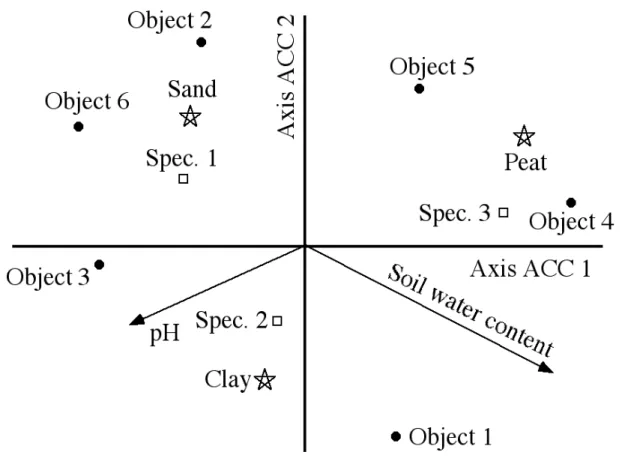
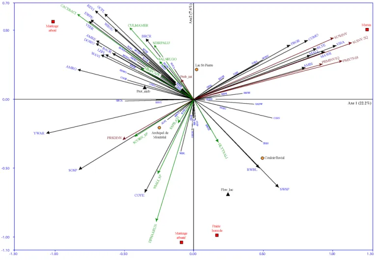
Figure 27 provides a fictitious example of a CCA triplot involving 6 objects, 3 species, 2 quantitative explanatory variables and one categorical explanatory variable with 3 states. Figure 28 is a real example of RDA biplot showing the two first axes of a canonical ordination of 143 sites, 63 Hellinger-transformed bird species abundances, 15 quantitative environmental variables and 9 classes of qualitative variables. This figure is here merely to show that a biplot can become rather crowded when the data set is large. In this case, the 143 sites were not represented on the scatterplot.

Figure 27: CCA triplot showing the objects (black dots), the response variables (species,

white squares), the quantitative explanatory variables (arrows) and the states of the qualitative explanatory variable (stars). Type 2 scaling: explanations in the text.

Figure 28 - Real example of RDA biplot (RDA on a covariance matrix, scaling 2) showing

the two first axes of a canonical ordination of 143 sites (not represented), 63 bird species (headless or full-headed arrows), 15 quantitative environmental variables (indented arrows) and 9 classes of qualitative variables (circles, squares and triangles).

4.7.4.1 Partial canonical ordination

In the same way as one can compute a partial regression, it is possible to run partial canonical ordinations. It is thus possible to run, for instance, an RDA of a (transformed) species data matrix (Y matrix), explained by a matrix of climatic variables (X), in the presence of edaphic variables (W). For instance, such an analysis would allow the user to display the patterns of species data uniquely attributed to climate when the effect of the soil factors are hold constant. The converse is possible also.

4.7.4.2 Variation partitioning

Borcard et al. (1992)1 _{devised a procedure called variation partitioning} in a context of multivariate ecological and spatial analysis. This method is based on (at least) two explanatory data sets. One explanatory matrix, X, contains the environmental variables, and the other (W) contains the x-y geographical coordinates of the sites, augmented (in the original paper) by the terms of a third-order polynomial function:

b0 + b1x + b2y + b3x 2 + b4xy + b5y 2 + b6x 3 + b7x 2 y + b8xy 2 + b9y 3

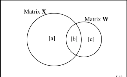
The procedure aims at partitioning the variation of a Y matrix of species data into following fractions (Figure 29):

[a] variation explainable only by matrix X

[b] variation explainable both by matrix X and matrix W [c] variation explainable only by matrix W

[d] unexplained variation.

Total variation of Y matrix

[a] [b] [c] Matrix X

Matrix W

[d]

Figure 29 - The fractions of variation obtained by partitioning a response data set Y with

two explanatory data matrices X and W.

1_{Borcard, D., P. Legendre. & P. Drapeau. 1992. Partialling out the spatial component of ecological}

Estimation of the R2 of the various components are obtained by first

computing the three following canonical ordinations: • Response data | Environment + Space : [a] + [b] + [c] • Response data | Environment : [a] + [b]

• Response data | Space : [b] + [c]

Beware: the R2 values obtained above are unadjusted, i.e. they do not take into account the numbers of explanatory variables used in matrices X and W. In canonical ordination as in regression analysis, R2 always increases when an explanatory variable x_i is added to the model, regardless of the real meaning of this variable. In the case of regression, to obtain a better estimate of the population coefficient of determination (ρ2), Zar (1999, p. 423)2, among others, propose to use an adjusted coefficient of determination:

R_adj2 =1− (n−1)

(n− m−1)(1− R

2

)

As Peres-Neto et al.3 have shown using extensive simulations, this formula can be applied to the fractions obtained above in the case of RDA (but not CCA), yielding adjusted fractions: ([a]+[b])_adj, ([b]+[c])_adj and ([a]+[b]+[c])_adj. These adjusted fractions can then be used to obtain the individual adjusted fractions:

4. Fraction [a]_adj is obtained by subtracting ([b]+[c])_adj from ([a]+[b]+[c])_adj.

5. Fraction [b]_adj is obtained by subtracting [a]_adj from ([a]+[b])_adj. 6. Fraction [c]_adj is obtained by subtracting ([a]+[b])_adj from

([a]+[b]+[c])_adj.

2

Zar, J. H. 1999. Biostatistical analysis. Fourth Edition, Prentice Hall, Upper Saddle River, NJ.

3

Peres-Neto, P. R., P. Legendre, S. Dray & D. Borcard. 2006. Variation partitioning of species data matrices: estimation and comparison of fractions. Ecology 87: 2614-2625.

7. Fraction [d]_adj is obtained by subtracting ([a]+[b]+[c])_adj from 1 (i.e. the total variation of Y).

We strongly advocate the use of the adjusted coefficient of

determination, together with RDA, for the partitioning of variation

of ecological data matrices.

This partitioning allows one to compute and test partial as well as

semipartial correlation coefficients. Note that these are computed on unadjusted fractions of variation.

The partial correlation of Y and X, controlling for W, is computed as r_{Y X.W} =

[ ]

[

]

[ ]

[ ]

(

)

The semipartial correlation of Y and X, in the presence of W, is computed as r_{Y (X .W )} =

[ ]

[

]

[ ]

[ ]

(

)

The coefficients of partial and semipartial determination are the squares of the correlation coefficients above.

These quantities are useful for testing purposes. Unbiased estimates of semipartial coefficients of determination, however, are computed as shown higher (adjusted R2).

If run with RDA, the partitioning is done under a linear model, the total SS of the Y matrix is partitioned, and it corresponds strictly to what is obtained by multiple regression if the Y matrix contains only one response variable. If run under CCA, the partitioning is done on the total inertia of the Y matrix (and runs into trouble when it comes to estimate unbiased values of the various fractions).

More recently, Borcard & Legendre (2002)4, Borcard et al. (2004)5 and Legendre & Borcard (2006)6 have proposed to replace the spatial polynom by a much more powerful representation of space. The method is called PCNM analysis. The acronym stands for Principal Coordinates of Neighbour Matrices. This technique will be addressed in Chapter 6.

It must be emphasised here that fraction [b] has nothing to do with

the interaction of an ANOVA! In ANOVA, an interaction is present

when the effects of one factor vary with the levels of another factor. An interaction can have a non-zero value and is easiest to detect and test when the two factors are orthogonal... which is the situation where fraction [b] is equal to zero! Fraction [b] arises because there

is some correlation between matrices X and W. It is not a testable

fraction and has no degrees of freedom of its own.

Note that in some cases fraction [b] can even take negative values. This happens, for instance, if matrices X and W have strong opposite effects on matrix Y while being positively correlated to one another.

When the [b] fraction is important with respect to the unique ([a]

and [c]) fractions, there is some uncertainty about the real

contribution of each explanatory matrix. This is so because fraction

[b] actually measures the degree of multicollinearity in the model. The more multicollinearity in a model the more unstable the regression coefficients are.

The variation partitioning procedure can be extended to more than two explanatory matrices, and can be applied outside of the spatial context. Function varpart of vegan allows the computation of partitionings involving up to 4 explanatory matrices.

4_{Borcard, D. & P. Legendre. 2002. All-scale spatial analysis of ecological data by means of principal}

coordinates of neighbour matrices. Ecological Modelling 153: 51-68.

5 _{Borcard, D., P. Legendre, Avois-Jacquet, C. & Tuomisto, H. (2004). Dissecting the spatial structures of}

ecologial data at all scales. Ecology 85(7): 1826-1832.

6_{Legendre, P. & D. Borcard. 2006. Quelles sont les échelles spatiales importantes dans un écosystème? In:}

4.7.5 Partial canonical ordination - Forward selection of environmental variables

There are situations where one wants to reduce the number of

explanatory variables in a regression or canonical ordination model.

Canoco and some functions in the R language allow this with a procedure of forward selection of explanatory variables. This is how it works:

1. Compute the independent contribution of all m explanatory variables in turn to the explanation of the variation of the response data table. This is done by running m separate canonical analyses.

2. Test the significance of the contribution of the best variable.

3. If it is significant, include it into the model as a first explanatory variable.

4. Compute (one at a time) the partial contributions (conditional effects) of the m–1 remaining explanatory variables, holding constant the effect of the one already in the model.

5. Test the significance of the best partial contribution among the m–1 variables.

6. If it is significant, include this variable into the model.

7. Compute the partial contributions of the m–2 remaining explanatory variables, holding constant the effect of the two already in the model.

8. The procedure goes on until no more significant partial contribution is found.

Stéphane Dray has written an R package (packfor) that allows to run RDA-based forward selection (function forward.sel). In Canoco 4.5, forward selection can be run either manually (at each step, the user asks for the test and decides whether to include a variable or not) or automatically. In the latter case, however, the program tests all the

variables and includes them all into the model, significant or not. The user has then to ask for the forward selection summary (FS summary button), examine the conditional effects and their probability, and rerun the analysis, retaining only the k first variables whose conditional effects are significant at a preestablished probability level.

Remarks

a) First of all, forward selection is too liberal (i.e., it allows to many explanatory variables to enter a model)

Before running a forward selection, always perform a global test

(including all explanatory variables). If, and only if, the global test is significant, run the forward selection.

Even if the global test is significant, forward selection is too liberal. Simulations have shown that, in addition to the usual alpha level, one must add a second stopping criterion to forward selection: the model under construction must not have an R2adj higher than

that of the global model (i.e., the model containing all explanatory variables)7. This second stopping criterion is available in the latest versions of the packfor package.

b) The tests are run by random permutations.

c) Like all procedures of selection (forward, backward or stepwise), this one does not guarantee that the best model is found. From the second step on, the inclusion of variables is conditioned by the nature of the variables that are already in the model.

d) As in all regression models, the presence of strongly intercorrelated explanatory variables renders the regression/canonical coefficients unstable. Forward selection does not necessarily eliminate this problem since even strongly correlated variables may be admitted into a model.

7

e) Forward selection can help when several candidate explanatory variables are strongly correlated, but the choice has no a priori ecological validity. In this case it is often advisable to eliminate one of the intercorrelated variables on an ecological basis rather than on a statistical basis.

f) If one wants to select an even larger subset of variables (and hence be even more liberal), another choice is backwards elimination, where one starts with all the variables included, and remove one by one the variables whose partial contributions are not significant. g) In cases where several correlated explanatory variables are present,

without clear a priori reasons to eliminate one or the other, one can examine the variance inflation factors (VIF), available as an R function written by Sébastien Durand, and provided in Canoco. The variance inflation factors (VIF) measure how much the variance of the canonical coefficients is inflated by the presence of correlations among explanatory variables. This measures in fact the instability of the regression model. As a rule of thumb, ter Braak recommends that variables that have a VIF larger than 20 be removed from the analysis. Beware: always remove the variables one at a time and recompute the analysis, since the VIF of every variable depends on all the others!

4.7.6 Distance-based redundancy analysis (db-RDA)

For cases where the user does not want to base the comparisons among objects on the distances that are preserved in CCA or RDA (including the species pre-transformations), another approach is possible for canonical ordination: db-RDA (Legendre & Anderson 1999)8. Described in the framework of multivariate ANOVA testing, the steps of a db-RDA are as follows:

8_{Legendre, P. & M. J. Anderson. 1999. Distance-based redundancy analysis: testing multi-species}

1. Compute a distance matrix from the raw data using the most appropriate association coefficient.

2. Compute a PCoA of the matrix obtained in 1. If necessary, correct for negative eigenvalues (Lingoes or Caillez correction), because the aim here is to retain all the data variation.

3. Compute an RDA, using the objects × principal coordinates as dependent (Y) matrix and the matrix of explanatory variables as X matrix.

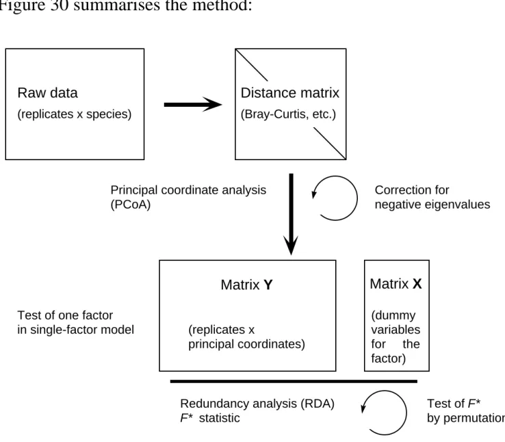
Figure 30 summarises the method:

Raw data

(replicates x species)

Distance matrix

(Bray-Curtis, etc.)

Principal coordinate analysis (PCoA) Correction for negative eigenvalues (replicates x principal coordinates) Matrix Y Matrix X (dummy variables for the factor) Test of one factor

in single-factor model

Redundancy analysis (RDA) F* statistic

Test of F* by permutation

Note that nowadays, thanks to the transformations proposed by Legendre & Gallagher (2001) for the species data matrices and allowing the direct application of RDA to species data, db-RDA is less used in this case.

4.7.7 Orthogonal factors: coding an ANOVA for RDA

As mentioned above, RDA is a linear method. It is the direct extension of multiple regression to multivariate response variables. On the other hand, ANOVA can be computed using a multiple regression approach if the factors and interactions are coded in an appropriate manner. Therefore, using the same coding, it is possible to run multivariate ANOVA using RDA, with great advantages over traditional MANOVA: there is no limitation about the number of response variables with respect to the number of objects; the ANOVA can be tested using permutations, which alleviates the problems of distribution of data (see further down); the results can be shown and interpreted with help of biplots. Furthermore, using the pre-transformations of species data, one can now compute MANOVA on species data. This is of great interest to ecologists, who use experimental approaches more and more.

The two following pages show how to code two orthogonal factors, without interaction first (when these is only one experimental or observational unit for each combination of the two factors) and with interactions (in the case of more than 1, here 2 objects per combination). This coding (called orthogonal contrasts or Helmert coding) works for balanced experimental designs.