Support vector machines to detect physiological patterns for EEG and EMG-based human-computer interaction:a review

Support Vector Machines to detect physiological patterns for

EEG and EMG-based Human-Computer Interaction: a review

1_{Department of Electronic Engineering, University of Rome Tor Vergata, Rome, Italy}

2 _{School of Life and Health Sciences, Aston Brain Center, Aston University, Birmingham, UK}

3 _{Department of Civil Engineering and Computer Science, University of Rome Tor Vergata, Rome, Italy}

Corresponding Author: Lucia R. Quitadamo

Email: [email protected] Telephone: +44-(0)121-2044103

Abstract

Support Vector Machines (SVMs) are widely used classifiers for detecting physiological patterns in Human-Computer Interaction (HCI). Their success is due to their versatility, robustness and large availability of free dedicated toolboxes. Frequently in the literature, insufficient details about the SVM implementation and/or parameters selection are reported, making it impossible to reproduce study analysis and results. In order to perform an optimized classification and report a proper description of the results, it is necessary to have a comprehensive critical overview of the application of SVM. The aim of this paper is to provide a review of the usage of SVM in the determination of brain and muscle patterns for HCI, by focusing on electroencephalography (EEG) and electromyography (EMG) techniques. In particular, an overview of the basic principles of SVM theory is outlined, together with a description of several relevant literature implementations. Furthermore, details concerning reviewed papers are listed in tables, and statistics of SVM use in the literature are presented. Suitability of SVM for HCI is discussed and critical comparisons with other classifiers are reported.

1. Introduction

Human-Computer Interaction/Interface (HCI) and Human-Machine Interface (HMI) consist of technologies that allow humans to control external peripherals or electronic devices. In order to achieve such control, humans can either interact with the devices by means of a “direct” medium, such as vision, hearing, touch, and gesture [1-4], or an “indirect” one, such brain or muscular activity. The indirect activity can be measured using techniques, such as ElectroEncephaloGram (EEG) and Electromyograms (EMG), which furnish data to be converted into commands for the peripherals. Specifically, EEG and EMG play a fundamental role in HCI, being the main source of data for driving electronic/electromechanical devices used to support disables’ life routines and rehabilitation. In particular, EEG can be the core of a special interface, that is, the Brain-Computer Interface (BCI) used by people who are paralyzed after a trauma or a degenerative disease [5, 6]. In addition, EMG can be the source signal for amputees to drive prostheses, artificial limbs or exoskeletons, so to recover missed limb functionalities by using residual muscles activity [7, 8].

Physiological signal-based HCIs have also found applications in non-strictly related medical fields, such as emotions recognition [9], smart home control [10], drivers' distraction avoidance [11] and musical expression [12].

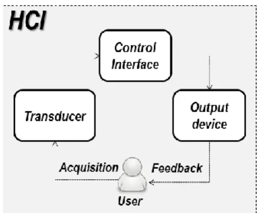
Independently from the input signal, a unique functional model is accepted to describe HCI systems, see figure 1 [13], made by the following components: 1) the acquisition, which concerns the signal measurement and data transmission; 2) the transducer, which is devoted to the extraction of the features, that are special characteristics of the measured signals, and to the recognition of the user’s intent, by means of a classification algorithm; 3) the control interface, which translates the classification output into a control command for the external device; 4) the output device, which is the peripheral to be driven. A visual, acoustic and/or tactile feedback is provided from the device back to the user in order to allow performance adjustments.

The core of the whole HCI chain is the detection of the patterns associated to the user’s volition: while the user must be trained at correctly performing the task, the classifier, that is a set of software routines, must be trained to correctly recognize the particular task among a set of others, which are the classes. For these reasons, many studies in the literature have been devoted to find classification algorithms with the accuracy as high as possible (see [14] for a review of classification techniques in EEG-BCIs and [15] for details about EMG classification). Among classifiers, Support Vector Machines (SVMs) have been widely implemented for HCI due to their versatility and robustness with non-stationary data [16]. Moreover, SVMs can be easy to implement even for non-experts, thanks to the availability of different free toolboxes for SVM-based classification, e.g. LIBSVM [17], SVM-light (http://svmlight.joachims.org/), SVMTorch [18], mySVM (http://www-ai.cs.uni-dortmund.de/SOFTWARE/ MYSVM/index.html), just to name a few, or to the many SVM implementations in Matlab (The MathWorks Inc., Natick, MA, 2000). However, if not fully understood, sometimes a non-optimal choice of the SVM parameters for the classification can be adopted. Moreover, many works lack in details on the setting of SVM, which are strategical in replicating the analysis and the results, as it occurs for research matters.

The objective of this review is to describe the use of SVMs in the HCI field, with the aim to provide

some practical hints for correct SVM-based classification. We limited the search to electrophysiological signal-based HCIs, in particular EEG and EMG-based, and mainly to HCIs used for device control. A description of the main theoretical aspects underlying SVMs is provided, including an overview of the mostly adopted SVM implementations, and details are tabled. A statistical analysis of the occurrences of SVM features in the literature is performed, including a critical comparison with other classifiers. Source bibliography comes from the main online databases, in particular Pubmed, Scopus, IEEE Xplore, up to year 2015. The list of all the main acronyms used in the manuscript can be found in Appendix A.

2. Introduction to SVM-based classification

For the sake of clarity, the following introduction to SVM will start from intuitive geometric concepts. Nevertheless, SVM classification has very strong theoretical bases in the theory of statistical learning developed by Vapnik and Chervonenkis [19].

2.1. Margin maximization

In machine learning, a classification problem consists in the identification, within a set of categories, of the category a new observation belongs to; such identification is performed on the basis of the information previously deducted from a set of observations whose category membership is known. The phase of information extraction is called training, while the phase of unknown instances categorization is called testing.

Let’s consider the binary classification problem depicted in figure 2, where squares denote objects belonging to class 1, and circles represent objects belonging to class 2. In principle, the separation in two classes can be realized by any line (in general infinite lines) that separates the two regions containing only squares and only circles, respectively, as the examples of line “A” or line “B” in figure 2. Intuitively, line “A” seems to realize a better separation between classes with respect to line “B”, since it separates with a safer margin, key concept of the SVM approach towards classification [20]. In the binary case, that is, the classification between only two classes, in a multiple-dimension space, SVM is used to find the hyperplane having the maximum distance (or margin) from both classes [21].

Regardless the class, the points closest to the hyperplane are called support vectors (black squares and circles in figure 2).

Let 𝑥𝑖 ∈ 𝑅𝑛, with 𝑖 = 1, 2, … 𝑁, be the 𝑖𝑡ℎ point of a set 𝑆, 𝑛 being the total number of features and R the space of the features; 𝑥_𝑖 can belong to class 𝜔₁ or to class 𝜔₂, which are assumed to be linearly separable. A hyperplane in 𝑅𝑛 _{can be written as 𝑤}𝑡_{𝑥 + 𝑤}

0= 0, where 𝑤 ∈ 𝑅𝑛 is an n-dimensional weight vector, and 𝑤₀ is a bias term. Many conventional hyperplane-based classifiers, e.g. Linear Discriminant Analysis (LDA) [22, 23], aim at finding optimal values for 𝑤 and 𝑤₀ so that 𝑤𝑡_{𝑥 + 𝑤}

0>

0 if 𝑥 belongs to class 𝜔1, and 𝑤𝑡𝑥 + 𝑤0< 0 if 𝑥 belongs to class 𝜔2 (the case 𝑤𝑡𝑥 + 𝑤0= 0 is a point of uncertainty and 𝑥 is typically assigned to one of the two classes arbitrarily). Differently, SVM does not only require that the training patterns lie on the correct side of the decision boundary, but also requires the safety margin, for a better generalization capability. In particular, during the training phase we require more stringent inequalities, such as:

𝑤𝑡_𝑥

𝑖+ 𝑤0≥ 1 if 𝑥𝑖 belongs to class 𝜔1 (1)

𝑤𝑡_𝑥

𝑖+ 𝑤0≤ −1 if 𝑥𝑖 belongs to class 𝜔2 (2)

which can be trivially satisfied by taking a large enough 𝑤. The maximization of the margin is obtained with the minimization of the norm of 𝑤, 𝐽(𝑤) = 1

2𝑤 ∙ 𝑤, while being bounded by the above constraints.

𝐽(𝑤) is called the objective function (1/2 is for computation convenience).

Finally, in the test phase, we classify the new instances according to the usual rules: If 𝑤𝑡_𝑥

𝑖+ 𝑤0> 0, then assign 𝑥𝑖 to class 𝜔1 (3) If 𝑤𝑡_𝑥

𝑖+ 𝑤0< 0, then assign 𝑥𝑖 to class 𝜔2 (4) It turns out that the above described optimization problem can be put in terms of a convex quadratic program and therefore: (i) it has a single global optimum and (ii) it can be solved using well-known techniques (see [24] for further details). In addition, this program has a number of relevant properties:

 Its complexity depends on the number of training instances only, i.e. the size of the training dataset, and not on the feature space dimensionality. This is a very important peculiarity of SVMs, which makes them insensitive to the so-called “curse of dimensionality”, a major concern when designing EMG and EEG-based systems [14]. The “curse of dimensionality” depends on the fact that, if the number of training data is small compared to the number of extracted features, the classifier will probably perform poorly due to insufficient data to build the classification rule. This curse affects mainly BCI systems as small training samples are usually available (training is consuming for the subjects) and many channels (and features) are needed to describe the classification problem.

 The weight vector 𝑤 depends only on the training patterns that lie on the margin (for those instances we have 𝑤𝑡_{𝑥 + 𝑤}

0= ±1), i.e. the support vectors.

 Given 𝑤, it is simple and straightforward to compute the bias parameter 𝑤0. 2.2. Non linearly separable data: the soft-margin

When data are not linearly separable, no hyperplane that perfectly discriminates classes exists. Consequently, we can find a hyperplane with the lowest error, as our best. In such an occurrence, two error sources are considered: misclassifications, i.e. points that lie on the wrong side of the hyperplane, and within-the-margin anomalies, i.e. points that lie on the correct side of the hyperplane but within the margin. To model those errors, a slack variable 𝜉_𝑖 ≥ 0 is introduced for each training instance 𝑥_𝑖. If 𝑥_𝑖

is correctly classified, then 𝜉𝑖 = 0. If 𝑥𝑖 lies within-the-margin or gets misclassified, then 𝜉𝑖 is set to the distance of 𝑥_𝑖 from the separating hyperplane. In this way, the constraints of the optimization problem become:

𝑤𝑡_𝑥

𝑖+ 𝑤0≥ 1 − 𝜉𝑖 if 𝑥𝑖 belongs to class 𝜔1 (5)

𝑤𝑡_𝑥

𝑖+ 𝑤0≤ −1 + 𝜉𝑖 if 𝑥𝑖 belongs to class 𝜔2 (6) and the sum of the slack variables, i.e. the overall error, is added as a penalty factor to the objective function. The resulting program can then be solved similarly to the linearly-separable data case [24]. Usually, a regularization parameter C is introduced to weight the penalty term in the objective function, which then becomes 𝐽(𝑤, 𝜉) = 1

2𝑤 ∙ 𝑤 + 𝐶(∑ 𝜉𝑖 𝑁

𝑖=1 ), thus allowing the experimenter to trade the training set accuracy off for the expected generalization capability. If a large value of C is chosen, then the resulting hyperplane will commit fewer errors on training data but will be characterized by a smaller margin (thus a minor expected generalization capability). On the contrary, a small value of C will lead to an SVM with greater expected generalization capability (larger margin) but misclassifying more training instances. The soft-margin implementation is advisable for EEG and EMG classification: in fact, both signals are often characterized by high levels of outliers and noisy examples, which can derive from artefacts (e.g. motion artefacts, equipment artefacts, etc.) and by a poor signal-to-noise ratio. The possibility to have adjustable margins which take into account the effect of outliers in the training dataset is definitively beneficial.

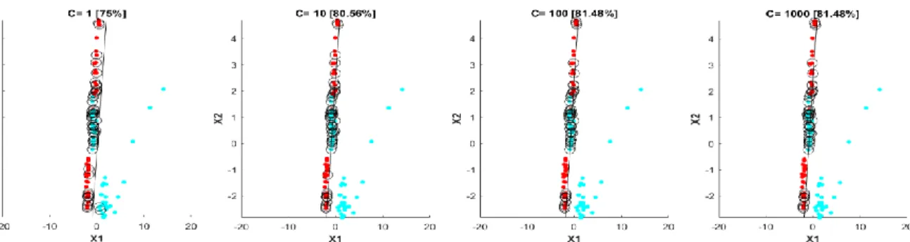
The choice of C is critical, leading to overfit or underfit risks for too high or too low values of C respectively, as schematically represented in figure 3. A binary classification problem is depicted. It can be easily seen how the choice of different values of C affects the number of support vectors and, definitively, classification performances, which range from 75% with C=1 to 81.48% with either C= 100 or C= 1000.

No optimal criteria are given to set a value for C, but grid-search and cross-validation can be considered, assigning values within 10−6_-10+6 _{on a logarithmic scale [24]. The introduction of the slack variables} simply softens the aforementioned margin, so that we can refer to soft margin SVM or C-SVM; it

Figure 3: Binary classification with a linear SVM and different values of C (1, 10, 100 and 1000). Red dots represent samples in class 1, cyan dots represent samples in class 2, and circles indicate support vectors. X1 and X2 represent the first two dimensions of the feature vector. Accuracy is reported in brackets. Data come from an EMG-based protocol, where the subject was asked to perform 5 different hand gestures (see [25] for details on protocol implementation and data analysis). For the sake of simplicity, just two tasks are considered.

represents the standard configuration for a typical SVM classification problem.

Even though the value of C can be associated to the extent of the margin, such a relationship is difficult to visualize and quantify. Therefore, it is worth considering another implementation of the soft margin concept, called 𝜈-SVM, which results in an easier interpretation, thanks to the introduction of parameters 𝜈 and 𝜌 [26], with 𝜈 ∈ [0,1] and 𝜌 ≥ 0. The penalty factor becomes:

−𝜈𝜌 +1 𝑁∑ 𝜉𝑖

𝑁 𝑖=1

(7) and the constraints:

𝑤𝑡_𝑥 𝑖+ 𝑤0≥ 𝜌 − 𝜉𝑖 if 𝑥𝑖 belongs to class 𝜔1 𝑤𝑡_𝑥 𝑖+ 𝑤0≤ −𝜌 + 𝜉𝑖 if 𝑥𝑖 belongs to class 𝜔2 (8) (9) The role of 𝜈 and 𝜌 can be figured out considering that when all instances lie on the correct side of the hyperplane, and outside the margin, 𝜉_𝑖 equals zero for all input data 𝑥_𝑖, and the constraints (8-9) reduce to 𝑤𝑡_𝑥

𝑖+ 𝑤0≥ 𝜌 and 𝑤𝑡𝑥𝑖+ 𝑤0≤ −𝜌. It follows that 2𝜌 ‖𝑤‖⁄ is the margin that separates the classes. In general, considering misclassifications and within-the-margin anomalies, 𝜌 is linearly related to the size of margin. In the occurrence of 𝜌 = 1, corresponding to the soft margin constraints, according to the eq. (7), the term (1 𝑁⁄ ) ∑𝑁 𝜉_𝑖

𝑖=1 represents the fraction of errors relative to the training data, while

𝜈 represents a sort of compensation: the higher the value of 𝜈, the lower the penalty factor. In other words, 𝜈 indicates the fraction of errors we can accept. It turns out that this interpretation is valid for any 𝜌 ≥ 0 and that 𝜈 represents both an upper bound on the fraction of errors (misclassifications and within-the-margin anomalies), and a lower bound on the fraction of input instances that will be selected as support vectors (see [27] for further details).

All considered, the 𝜈-SVM allows a more evident and direct interpretation of the parameters with respect to C-SVM, but needs the optimization of two variables (𝜈 and 𝜌) instead of one (C).

2.3. Non linearly separable data: the kernel trick

Soft-margin admits a certain error so to allow a linear approach for non-linearly separable data. Such an approach is useless in case the separating function is “inherently” non-linear, so that it is worth to consider the option of projection. In fact, data not-linearly separable in their original space can get linearity when mapped into another one (especially when of higher dimensionality), so that SVM can be further applied.

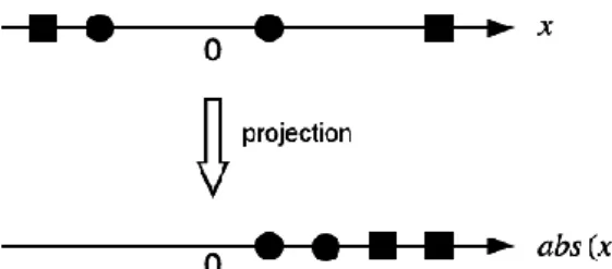
Figure 4: Space Projection. The two classes, circles and rectangles, are non-linearly separable in the original space (the top arrow), but become linearly separable in another space provided by the abs(-) function (the bottom arrow).

As an example, figure 4 shows four mono-dimensional instances belonging to two classes (circles vs. rectangles). In the original space (top row), no single point separates the two classes, but the abs(-) function provides mapping into another space allowing linear separation between classes (bottom row). Let 𝜙 ∶ 𝑅𝑛_{→ 𝐻 denote the mapping function. Firstly, each input instance 𝑥}

𝑖 is mapped according to

𝜙(𝑥_𝑖). Then we train our SVM model, typically using a soft-margin formulation, to discriminate the mapped points. Adopting the quadratic program computations [24], the training algorithm will depend on 𝜙 only trough dot products of mapped instances, i.e. 𝜙(𝑥_𝑖) ∙ 𝜙(𝑥𝑗). Since there must exists a function

𝐾: 𝑅𝑛_{× 𝑅}𝑛_{→ 𝑅 such that 𝐾(𝑥}

𝑖, 𝑥𝑗) = 𝜙(𝑥𝑖) ∙ 𝜙(𝑥𝑗), it is sufficient to use 𝐾 in the training algorithm, avoiding computing the mapping functions 𝜙(𝑥_𝑖) and 𝜙(𝑥𝑗) explicitly. 𝐾 is known as the kernel function, while the whole procedure is known as the kernel trick, as it allows advantages of the mapping procedure without higher computational costs. The fact that the decision rule of SVM is a simple linear function in the kernel space makes SVM stable and characterized by low variance (variance reflects the sensitivity of the classifier to the training set used [14]). This is a useful property when dealing with EEG and EMG data, which are non-stationary signals with features changing over time; low-variance classifiers, such as SVM, can cope with such signals better than others.

A valid kernel function has to be positive definite (Mercer’s condition), symmetric, and has to reflect the similarity between its inputs, i.e. 𝐾(𝑥𝑖, 𝑥𝑗) should be high (low) if 𝑥𝑖 and 𝑥𝑗 are similar (dissimilar) with respect to the problem at hand [20].The most used kernels are:

 Radial Basis Function (RBF), 𝐾(𝑥𝑖, 𝑥𝑗) = 𝑒− ‖𝑋𝑖−𝑋𝑗‖2 2𝜎2 , 𝜎 ≠ 0.  Polynomial, 𝐾(𝑥𝑖, 𝑥𝑗) = (𝑥𝑖∙ 𝑥𝑗+ 1) 𝑑 , 𝑑 > 0.  Sigmoidal, 𝐾(𝑥𝑖, 𝑥𝑗) = tanh(𝑘𝑥𝑖∙ 𝑥𝑗− 𝛿).  Cauchy, 𝐾(𝑥𝑖, 𝑥𝑗) = (1 +‖𝑥−𝑦‖ 2 2𝜎2 ) −1 , 𝜎 ≠ 0.  Logarithmic, 𝐾(𝑥𝑖, 𝑥𝑗) = − log(‖𝑥 − 𝑦‖𝑑+ 𝑐), 𝑑 > 0.

The linear problem can be considered as a subset of the non-linear one with kernel 𝐾(𝑥𝑖, 𝑥𝑗) = 𝑥𝑖∙ 𝑥𝑗. For each kernel choice, the values of other parameters, besides C, should to be set. For example in the popular RBF kernel the experimenter has to choose also the kernel width 𝜎. To do so, the grid-search is usually adopted; anyway other techniques, such as Particle Swarm Optimization (PSO) [28] and Genetic Algorithms (GA) [29] are also used in the literature.

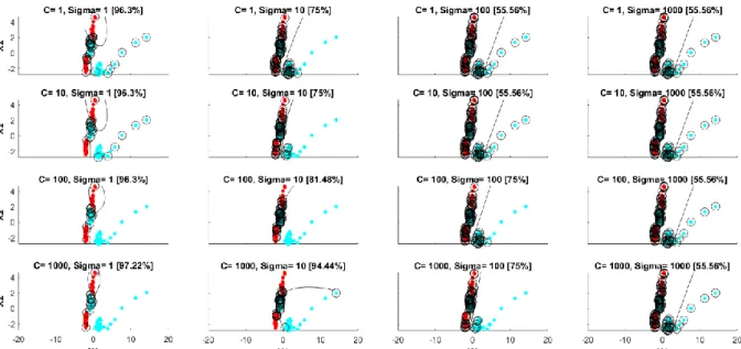
Values determined for the kernel and the related parameters greatly influence the decision surface and, consequently, the classification performance. In figure 5 and for the same dataset used for figure 3, an RBF kernel is optimized considering for both C and 𝜎 values of 1, 10, 100 and 1000. According to the results, the selection of C=1000 and 𝜎=1 allows an accuracy as high as 97.22%. In figure 6, instead, the results of the optimization of a polynomial kernel-SVM with degree d are reported, considering for C values of 1, 10, 100 and 1000 and for d values of 2, 5, 7 and 10. As a result, the highest accuracy (97.22%) is obtained both with C=1000, d=2 and with C=1000, d=7. In case of equal accuracies, the time spent for the training can be used as a metric to choose the most performing configuration.

Figure 5: Binary classification of EMG data with an SVM with RBF kernel. C and 𝜎 can be 1, 10, 100 and 1000. Red dots represent samples in class 1, cyan dots represent samples in class 2, and circles indicate support vectors. X1 and X2 represent the first two dimensions of the feature vector. Accuracy is reported in brackets. Data come from an EMG-based protocol, where the subject was asked to perform 5 different hand gestures (see [25] for details on protocol implementation and data analysis). For the sake of simplicity, only two tasks are considered.

Figure 6: Binary classification of EMG data with an SVM with polnomial kernel. C can be 1, 10, 100 and 1000, while the degree (d) of the polynomial can be 2, 5, 7 and 10. Red dots represent samples in class 1, cyan dots represent samples in class 2, and circles indicate support vectors. X1 and X2 represent the first two dimensions of the feature vector. Accuracy is reported in brackets. Data come from an EMG-based protocol, where the subject was asked to perform 5 different hand gestures (see [25] for details on protocol implementation and data analysis). For the sake of simplicity, only two tasks are considered.

2.4.Multiclass SVM

In principle, the margin criterion of SVM can perform multi-class classification but it is useless, resulting in a quadratic program with too many variables to be optimized. Differently, more computationally efficient techniques, although potentially inaccurate, are typically used in order to build a multi-class SVM starting from many 2-class SVMs [22, 24], namely One-Vs-One (OVO) (also called in the literature Against-One (OAO)) and the Vs-All (OVA) (also called in the literature One-Against-All (OAO) and One-Against-Rest (OAR)).

For OVO, the 𝑀-class problem is split into 𝑀(𝑀 − 1) 2⁄ binary problems aimed at separating one class from another. To obtain the final response, i.e. the class to which a new input instance is expected to

belong, a majority voting strategy is employed.

For OVA, 𝑀 classifiers are built. The task of the 𝑖-th (𝑖 = 1, … , 𝑀) classifier is to separate the instances belonging to class 𝑖 from all the others. When a new input has to be classified, every classifier is asked for its corresponding score and the class having the highest result is selected as the final response. All those strategies can have the drawbacks to determine unclassifiable/uncertain regions in the feature space, and to meaningfully increase the computational time with the number of classes. In order to overcome such limitations, the Directed Acyclic Graphs (DAG) approach, consisting in assigning unclassifiable regions to the classes associated with the leaf nodes of a decision tree, was suggested [30].

2.5.SVM variants

In view of the intrinsic limitations of each of the aforementioned approaches, many variants of SVM have been developed; the most relevant for our purposes are:

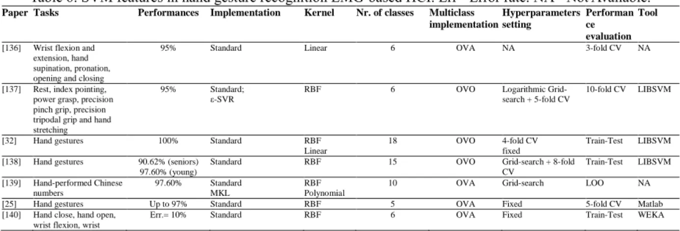
 Least-Squares SVM (LS-SVM): differently from solving a quadratic programming problem with linear inequality constraints with standard SVM, LS-SVM involves solving a set of linear equations, thus making the solution less time-consuming in the presence of large training sets [31]. Large datasets are typical of EMG-based studies, where a huge number of classes is usually taken into account (e.g. 18 different hand gestures in [32]) and to a minor extent of BCI protocols which usually involve less classes (2 to 5).

 Fuzzy SVM (FSVM): allows integrating in SVM a means for assigning a utility value to the training data [33]. Indeed, in many real-world applications, some of the training instances could be more important than the others, and the learning algorithm should take into account this difference. This is useful when the training set is suspected of containing outliers and/or mislabeled points, a condition typical of both EEG and EMG data which are highly sensible to different sources of noise.

 Fuzzy Least-Squares SVM (FLS-SVM): overcomes the issue of unclassifiable regions in the feature space, which can occur with standard SVM or LS-SVM in solving multiclass problems by means of the OVO or the OVA approach [34]. This advantage can be obtained using learner-specific fuzzy membership functions, combinable to obtain (fuzzy) class-specific membership functions that are well-defined in each portion of the feature space. This implementation can be very useful when dealing with EMG-based datasets, which usually contain a huge number of classes.

 Multiple Kernel Learning SVM (MKL-SVM): the kernel function becomes a linear or nonlinear combination of multiple base kernels [35]. Consequently, data can come from non-homogeneous information sources. Moreover, the optimal combination is itself learned from data, thereby eliminating the need for a preliminary, possibly arbitrary, kernel selection. This can be very useful for reducing variance in the problem and making SVMs more stable, a property that allows them to cope with non-stationary data such as EEG and EMG.

 Spatially-weighted SVM (sw-SVM): proposes to integrate spatial feature weights into the SVM optimization problem and to tune these weights as if they were hyperparameters [36]. In this way the classifier learns from spatially filtered data, thus improving class separation, while reducing errors. This implementation allows to enhance just the weight of the most informative channels and can be efficient in case of high-density datasets, typical of EEG recordings.

 K-means SVM: a 𝑘-means procedure can be implemented before SVM classification in order to avoid possible shortcomings due to input data redundancy and to speed up training [37]. Clusters containing only vectors belonging to the same class can be disregarded, while the others are retained and considered. SVM training is then carried on the new reduced training dataset, with a noteworthy reduction of complexity. This could be a valuable property when dealing with the classification of large datasets, such as the EEG and EMG ones.

 Relevance Vector Machine (RVM): it can overcome some of the typical limitations of SVMs (e.g. determination of the C parameter, non-probabilistic predictions) [38]. RVMs have the same functional form of SVMs but within a Bayesian framework.

 Twin SVM: uses two different SVMs, one for each class, for binary problems, and generates two distinct hyperplanes, each one being close to the patterns of the relative class, “1” outdistanced from the point of the other class. The class of a point 𝑥 is determined by the closest hyperplane.

Twin SVM allows a smaller number of constraints with respect to a standard SVM, and enhances operational speed [39], a property valuable for online implementations of HCI systems.

 ε-Support Vector Regression (ε-SVR): SVMs can be used also for regression [40]. The task of 𝜀 -SVR is to find a continuous function 𝑓(𝑥) that has at most 𝜀 deviation from the actual targets of data samples and is as flat as possible. This is equivalent to estimating regression coefficients of

𝑓(𝑥) with these requirements. It can happen that the linear function 𝑓 is not able to fit the training data. Hence, as for the classification case, slack variables 𝜉 (and therefore C) or kernels can be introduced.

2.6. Performance Evaluation

The performances of SVMs, and of classifiers in general, are usually evaluated by means of accuracy (or success rate or recognition rate), defined as the number of correct classifications over the total classifications. They can also be expressed in terms of error rate (or misclassification rate), defined as

(100 − 𝑎𝑐𝑐𝑢𝑟𝑎𝑐𝑦)% and representing the number of errors over the total classifications. If a classifier is not able at distinguishing the classes, its performances equate the chance level (50% of accuracy in a binary problem).

Different methods can be used to evaluate accuracy:

 Train-Test evaluation: consists in randomly or sequentially splitting the whole dataset into a training and a testing set and in computing accuracy on the testing set.

 N-fold Cross Validation (CV): consists in partitioning the whole dataset in 𝑁 not-intersecting subsets, approximately of the same size, and in using the ith _{subset as a testing set and the remaining}

𝑁 − 1 subsets as training set; the process iterates until each subset is used once as a testing set, and the accuracy comes from the average of the 𝑁-tests accuracies.

 Leave-One-Out (LOO) CV: consists in leaving one sample out of the whole available dataset to build the testing set and using all the remaining samples as training set; the process iterates until each sample of the dataset is used once as a testing set.

CV is more computationally demanding than train-test, but allows to have an unbiased performance estimate, since all data are used (at least once) for testing; in this way the performance is independent from the particular dataset division which is adopted.

When accuracies of different classifiers need to be compared and statistical significance among different classifiers needs to be assessed, confidence intervals and statistical tests can be used [41]. Although these methods are well-founded and can provide the experiment with more reliable estimates, they are rarely used in HCI studies because of the huge amount of data necessary for meaningful results. Even if widely used, accuracy has some limitations as an evaluation criterion, as it does not take into account the class distribution among examples (e.g. less frequent classes have smaller weight in the total accuracy) and the loss of information due to different types of errors (e.g. did the classifier misclassify the class or simply abstain from classification? [42]). For these reasons, many indicators can be introduced in order to have a more realistic evaluation of the whole classification process (e.g. sensitivity, specificity, precision, recall, Cohen’s kappa coefficient, Area under Roc Curve (AUC), etc.). The interested reader can refer to [43] for a generic overview of evaluation criteria in machine learning and to [44] for an overview of performance evaluation in BCI and HCI in general.

3. EEG-based HCI and SVM

3.1. Overview of BCI systems

BCIs rely on the recording of user-modulated brain signals to drive a device. Brain signals can be measured by means of different technologies either invasive, such as the ElectroCorticoGraphy (ECoG) [45] or non-invasive, such as the EEG [46], the functional Near-Infrared Spectroscopy (fNIRS) [47], the MagnetoEencephaloGraphy (MEG) [48] , the functional Magnetic Resonance Imaging (fMRI) [49], etc.

In this paper we focus on EEG-based BCIs, since they are popular for device control, thanks to the manageability and relatively low cost of the EEG technique. Anyway the interested reader can refer to the many reviews devoted to BCI (e.g. [50] for a complete review of processing algorithms for fNIRS-BCIs or [51] for a review of ECoG-based fNIRS-BCIs) to have a deeper understanding of the other techniques. Many brain patterns have been used and many protocols have been implemented for BCI. The most

studied ones are based on Event-Related Potentials (ERPs), which consist in brain responses evoked by external stimulations when the user performs a specific mental activity. This activity could be, for example, the mental discrimination of a rare acoustic stimulus in a set of frequent stimuli, the discrimination of a verbal incongruity or of a known face among anonymous ones, etc. These cognitive tasks evoke in the EEG a specific ERP response, which can be discriminated by means of algorithms and used to control a device. The most relevant application of ERP-based BCIs is the P300-speller [52, 53]. A subject is asked to focus the attention on a particular symbol in a matrix of symbols whose rows and columns iteratively flash. Three hundred milliseconds after the flashing of the row/column containing of the chosen symbol, a positive voltage spike, named P300, is measured on the subject’s scalp. When the P300 occurs, the classifier recognizes the symbol, so allowing the subject to communicate. Other than a symbol, ERP-based BCIs were used to recognize an intention of movement to drive a wheelchair [54], to drive an analogue mouse [55], a mobile robot [56], a domotic interface [57], to surf on the internet [58], to paint [59], to browse photographs [60], etc.

The control of a device can be also realized by means of Sensorimotor Rhythms (SMRs)-based BCI, on the basis of brain signal variations evoked by actual or imagined mental tasks [61]. When a subject moves or imagines to move a body segment or to perform a specific mental task, alpha (8-13Hz), beta (14-26Hz) and gamma (>30Hz) frequency bands, recorded on the brain sensorimotor cortex, vary in voltage amplitude (the first two increasing and the third decreasing). After a training stage, the subject learns how to voluntarily modulate those voltages and thus control a device, e.g. a helicopter in a 3D space [62], a cursor on a screen [46], a robotic arm [63], a wheelchair [64], a spelling program [65], etc. The third big class of BCIs is based on Steady-State Visually Evoked Potentials (SSVEP), which are responses evoked in the EEG spectrum by long trains of flickering visual stimuli and characterized by a frequency peak at the same frequency of the stimuli themselves. Being easily recognizable in the EEG spectrum, SSVEPs have been widely used to implement BCIs, with high accuracy and throughput rates, devoted e.g. to the selection of buttons on a screen [66], to the communication by means of a speller [67], to the driving of a wheelchair [68], to the control of a robotic arm [69], etc.

Finally, there is a class of BCI systems making use of Slow-Cortical Potentials (SCPs), which are slow (<1Hz) negative or positive potential shifts voluntary modulated by a subject to implement a binary communication [70]. SCPs-based BCIs have not found a wide diffusion for communication and control purposes, due to the slowness of brain responses, but were exploited for implementing neuro-rehabilitation strategies [71].

The following sections concern the review of the BCI literature, focusing on the exploited brain feature: ERPs, SMRs, SSVEPs and SCPs. Details of the SVM implementation and its performances are reported, making a comparison with those of other classifiers. The BCI protocol, the system and the applications are run over or just mentioned for the sake of simplicity.

3.2. Event-Related Potentials (ERPs)-based BCI systems

For typical speller-based applications, SVM was successfully adopted in [72], where a self-training semi-supervised linear-kernel SVM achieved an accuracy similar to that of a standard SVM (up to 98.5%) by using a smaller training dataset. In [73] an ensemble of linear SVMs achieved the same accuracy of a standard SVM, 96.5%, with the full training set, and accuracy higher by 5% with 1/3 of the training set. In [74] a sequential updating self-training LS-SVM, whose kernel gradually improved with the insertion in the training set of upcoming unlabeled data, was used with an online spelling accuracy greater than 85%. In [75] data from a P300 speller, with modifications in symbols size, symbols distances and speller colors, were classified with an RBF-SVM and an LDA, with RBF-SVM performing better in each condition (in the best configuration, accuracy up to 90% was achieved by SVM vs. 80% of LDA).

In ERPs-based protocols different from the speller one, as the one in [36], spatio-temporal filtering and an ensemble of linear sw-SVMs were used to classify data acquired from a visual feedback experiment, consisting in memorizing the position of a set of digits and in indicating the exact position of a random target number. The obtained classification accuracy was 87.80%±3.63%, higher than the ones achieved by linear SVM and simple sw-SVM (70.71%±10.77% and 80.71%±6.61%, respectively). In [76] authors compared an RBF-SVM against a linear SVM and a Linear Logistic Classifier (LLC) in classifying ERPs acquired during an image Rapid Serial Visual Presentation (RSVP) protocol. SVMs outperformed LLC, while RBF-SVM was more accurate than linear-SVM. In [77] ERPs following true

and false statements were classified with the aim to separate covert "yes" from covert "no"-thinking. Four classifiers were compared, namely a linear SVM, an RBF-SVM, a stepwise LDA and a shrinkage LDA. All the classifiers performed at chance level when separating "yes" from "no"; however, when the single responses were discriminated against baseline, RBF-SVM showed the highest accuracy (68.8%). In [9] a non-verbal communication-based BCI was created on the basis of the ERP associated to implicit negative emotional responses to specific neutral faces. SVMs were used with both linear and RBF kernels, with features both in time and time/frequency domains. The classifiers exhibited accuracy up to 80% in discriminating emotional responses. In [78] the imagination of Japanese vowels vocalization was investigated as an input to control a speech prosthesis. An RBF-SVM, a linear RVM (RVM-L) and an RVM with Gaussian kernel (RVM-G) were compared. Accuracy obtained by RVM-L was around chance level and also significantly worse than RVM-G’s one. Linear classification was ineffective for silent speech. In comparison to SVM-G, RVM-G achieved slightly better accuracy but with a significant reduction of relevant vectors, while its accuracy worsened in case of few training points.

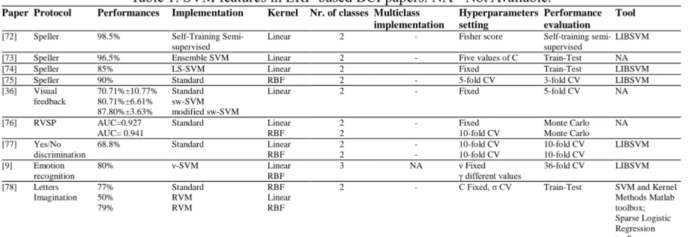
Table 1 summarizes the main SVM features used in ERPs-BCI works, namely, type of protocol, maximum achieved performances, SVM implementation, type of kernel, number of classes involved in the classification, type of multiclass implementation, adopted methodology to set hyperparameters, chosen methodology to evaluate performances, used tool. In particular, performances refer to the best obtained result, in terms of accuracy, or error rate, or AUC, etc. If not differently indicated, performances correspond to accuracy. In any case, a comparison among performances of different systems cannot be directly evidenced since the different implementations used.

Table 1: SVM features in ERP-based BCI papers. NA= Not Available.

Paper Protocol Performances Implementation Kernel Nr. of classes Multiclass implementation Hyperparameters setting Performance evaluation Tool

[72] Speller 98.5% Self-Training Semi-supervised

Linear 2 - Fisher score Self-training

semi-supervised

LIBSVM

[73] Speller 96.5% Ensemble SVM Linear 2 - Five values of C Train-Test NA

[74] Speller 85% LS-SVM Linear 2 Fixed Train-Test LIBSVM

[75] Speller 90% Standard RBF 2 - 5-fold CV 3-fold CV LIBSVM

[36] Visual feedback 70.71%±10.77% 80.71%±6.61% 87.80%±3.63% Standard sw-SVM modified sw-SVM

Linear 2 - Fixed 5-fold CV NA

[76] RVSP AUC=0.927 AUC= 0.941 Standard Linear RBF 2 2 - Fixed 10-fold CV Monte Carlo Monte Carlo NA [77] Yes/No discrimination 68.8% Standard Linear RBF 2 2 - - 10-fold CV 10-fold CV 10-fold CV 10-fold CV LIBSVM [9] Emotion recognition 80% ν-SVM Linear RBF 3 NA ν Fixed

γ different values 36-fold CV LIBSVM [78] Letters Imagination 77% 50% 79% Standard RVM RVM RBF Linear RBF

2 - C Fixed, σ CV Train-Test SVM and Kernel

Methods Matlab toolbox; Sparse Logistic Regression toolbox

Table 1 evidences that SVM, either with linear or RBF kernel, achieves high accuracy in ERPs discrimination and near 100% accuracy in speller applications. The implementations different from the standard C-SVM (sw-SVM for example) can boost ERPs-based BCI system performances, accordingly to the type of data and the final application. Hyperparameters setting is performed in different ways, mainly by fixing their values or by using CV. CV remains the method of choice for performance evaluation. As a final remark, LIBSVM results to be the most used toolbox.

3.3. Sensor-motor rhythms (SMRs)-based BCI

The SMRs-based BCI review regards papers dealing with different mental tasks which can be pure motor tasks, both motor and non-motor tasks and other typologies of tasks.

3.3.1. Motor tasks

The imagination of left and right hand movements is widely used in BCI, because such tasks evoke highly discriminable patterns in well-defined and opposite sides of the brain. For these reasons, many studies have tried to find the best combination of extracted features and classifier to boost their detection performances. For example, spatial and temporal Principal Component Analyses (PCA) and a linear SVM were used in [79] with accuracy of 73.65%, while in [80] an RBF-SVM outperformed five different classifiers (Linear Mahalanobis Distance, Quadratic Mahalanobis Distance, Bayesian Classification, two types of Artificial Neural Networks (ANN)) independently from the spatial and the

temporal filter used for the preprocessing. Also in [81] three different feature-extraction methods and three different classifiers (LDA, Adaboost and RBF-SVM) were compared, with SVM and LDA performing better (error rates of 0%-23.81% and 9.61%-14.33%, with SVM and LDA respectively) both with single features and with combinations of features. In [82] RBF-SVM outperformed LDA and ANN either with the proposed features (9% vs. 10% of ANN and 12% of LDA) and with simple AR features (18% vs. 21% of ANN and 22% of LDA). In [83] an RBF-SVM and a fuzzy RBF-SVM were compared with ANN and LDA and outperformed them in terms of amount of information transmitted per second. In [84] an RBF-SVM was used in combination with neuro-fuzzy prediction and multi-resolution fractal feature vector, with accuracy of 91%. In [85] authors proposed a kernel fisher (KF)-posterior-probability (PP)-SVM, consisting in calculating the within-class scatter matrix of the two classes, in integrating it into the RBF kernel of an LS-SVM, and in calculating the output of the classification with posterior probabilities. When compared to a simple SVM, a PP-SVM and a KF-SVM, the KF-PP-SVM achieved higher accuracy (75.73% vs. 70.86%, 71.52% and 74.11%). Finally, in [86] a feature selection technique, based on genetic algorithm (GA) and an RBF-SVM, resulted with accuracy higher than that obtained with feature combination (80.8% vs. 72.3%). With the adoption of GA, SVM showed higher accuracy with respect to ANN (80.8% vs. 75.6%).

In some studies, the imagery of feet movements was used together to other mental tasks, as in [87] where a linear SVM was compared to LDA, Mahalanobis Distance, Generalized Distance Based classifier and Bayes classifier, in the discrimination of left hand, right hand, feet and tongue movements. Accuracy higher than 80% was achieved by both LDA and SVM. Similarly, right foot imagery was classified in [88], where authors compared a Bayesian LDA (BLDA) with two different versions of LDA (simple and regularized) and with an RBF-SVM, with BLDA resulting the most accurate classifier. In [89] authors classified two datasets, which are right-hand/right-foot motor imagery and left-hand/right-foot motor imagery, with cross-correlation feature extraction and LS-SVM with RBF kernel. A logistic regression classifier and a kernel logistic regression classifier were used for comparison. LS-SVM achieved higher success rates than the two logistic regression classifiers (first dataset: 95.72%±4.35% vs. 89.54%±8.61% and 93.38%±6.76%; second dataset: 97.89%±2.96% vs. 95.31%±5.88% and 94.87%±6.98%). In [90] a PCA-based feature selection and RBF-SVM allowed discriminating data from two different datasets, including right-hand and foot motor imaginary and left-hand and foot motor imagery, with accuracies ranging from 61.36% to 90.63%. In [91] movement-related independent components and RBF-SVM were used for the classification of left-hand, right-hand and foot motor imagery, with accuracy of 65%. In [92] authors proposed a method based on spatial filtering and “classifiability” of features for the classification of two different datasets, one consisting of left-hand, right-hand, foot and tongue motor imagery and one of left-hand and right-hand motor imagery, by means of both standard SVM and twin SVM with RBF kernel. For binary classification, accuracy with twin SVM increased by up 20% with respect to the one obtained by standard SVM. In the multiclass case, accuracy was significantly higher when using twin SVM (up to 79%±5.8% in one subject) against SVM (49%±8.8%). In [93] authors introduced multiclass posterior probability for twin SVM in order to classify both several datasets of motor imagery tasks, made of different classes (from 3 to 11) and a dataset from BCI competitions (left-hand, right-hand, feet, tongue, http://www.bbci.de/competition/). Twin SVM performed with less computational time and higher accuracy with respect to SVM, especially with fewer samples. In [94] authors applied an optimal allocation-based approach for a discriminative feature extraction to data from binary motor imagery datasets (right-hand vs. right-foot and left-hand vs. right-foot) and used LS-SVM with RBF kernel and a Naïve Bayes for classification. LS-SVM performed better than Naïve Bayes (accuracy of 90.60%±11.31% and 96.62%±3.72% vs. 75.56%±22.35% and 96.36%±2.32%, with 6 and 11 features respectively). In [95] authors optimized Common Spatial Patterns (CSP) computed on multiple signals filtered at a set of overlapping bands, and used RBF-SVM in order to discriminate the imagination of right-hand and foot and of right-hand and left-hand. Results showed a lower error rate when an optimized filter was used (7.95%±2.45% vs. 13.33%±2.92% of simple CSP in the first dataset; 18.83%±3.55% vs. 23.10%±5.04% of simple SVM in the second dataset). In [96] the imagination of two different motor tasks (slow and fast right-arm flexion) and error potentials were classified by means of two linear SVMs with an average error rate lower by 14% than the case with no error potentials. The imagination of wrist extension was classified in [97], with a linear SVM used for recursive feature elimination and LDA for classification.

Besides classical motor imagery patterns, also parameters related to the imagined movements were discriminated, as in [98], where a wavelet-based feature extraction and an RBF-SVM were used to classify brain signals generated by variations of force-related parameters, during four different

voluntary tasks. The error rate provided by RBF-SVM, when compared with a simpler classifier (nearest representative classifier, NR), was significantly lower (15.8% in the best SVM case versus 40.2% in the best NR case). In [99] authors investigated the discriminability of real and imaginary isometric plantar-flexion of the right-foot at different target torques (TT) and at different rates of torque development (RTD), by using wavelets for feature extraction and an RBF-SVM for classification. Results showed that the TTs under ballistic and moderate RTD were discriminated with error rates of 16%±9% and 26%±13% respectively, while RTDs under high and low TT were discriminated with error rates of 16%±11% and 19%±10%, respectively, thus indicating the possibility to detect task parameters in single-trial EEG.

Finger movement imagery was widely used in SMR-based BCI, as in [100] where authors combined different spatio-temporal brain patterns, different spatial filtering and a linear SVM to discriminate left and right-hand fingers movements, with an accuracy higher than 85%. In [101] an SMR-BCI based on the discrimination of right-index finger lifting versus left-index finger lifting tasks was proposed. Four different classifiers were compared, namely a Fisher’s LDA, two types of ANN and an RBF-SVM which was the best performing classifier on average. In [102] the author used two different datasets, one consisting in the imagination of left- and right-hand movements and one in left- and right-finger lifting movements, and implemented a wavelet-based methodology to localize brain responses in the time-frequency domain, a fractal feature extraction and an RBF-SVM classification. Also he compared SVM-RBF with LDA and demonstrated the former to be more accurate than the latter (82.5% vs. 78.7%). Finger movements were also discriminated in [103] by using RBF-SVM, with an average accuracy of 77.11% in detecting movements on all possible couples of fingers. In [104] authors proposed Artificial Bee Colony (ABC) for feature selection in order to discriminate left and right finger lifting. Different features were extracted and both GA and ABC were used for selecting the best feature set. An RBF-SVM was used for classification. Average accuracy was 88.8% with ABC and 83.1% with GA. In [105] authors implemented a method for the recognition of real and imagined finger movements. Numerical and symbolic signal regression procedures were used for feature extraction in order to avoid the loss of information regarding the time localization of features. Then ANN and an RBF-SVM were used for classification. Results showed that SVM accuracy increased with the increasing of the number of trials (from 45% to 62%), while ANN performed better at single-trial discrimination.

Finally a new couple of motor imagery tasks, swallowing and tongue protrusion, was analyzed in [106] for post-stroke dysphagia rehabilitation. Features based on dual-tree complex wavelet transform and a linear SVM were used for classification. Results showed that average accuracies of 70.89% and 73.79% could by achieved when swallowing and tongue-protrusion were classified against idle state in healthy subjects. Also accuracy of 66.40% for swallowing and 70.24% for tongue protrusion were obtained with data from a stroke patient. Finally authors demonstrated that swallowing could be detected from tongue protrusion-models due to the high correlation between their classification accuracies.

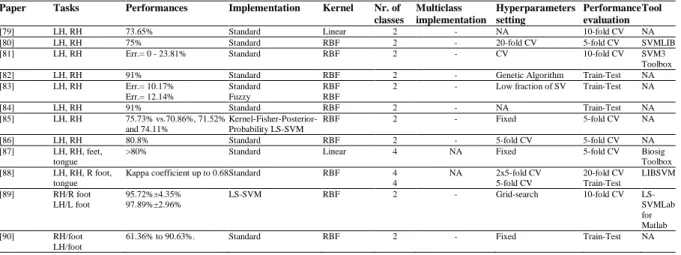
Table 2 summarizes the main SVM features of motor imagery-based BCI works. Differently from ERP-based papers, the second column of the table lists the tasks performed by the subjects rather than the specific protocol.

Table 2: SVM features in motor tasks-based SMR-BCI. L= left, R= right, H= hand. Err= Error Rate. NA= Not Available.

Paper Tasks Performances Implementation Kernel Nr. of classes Multiclass implementation Hyperparameters setting Performance evaluation Tool

[79] LH, RH 73.65% Standard Linear 2 - NA 10-fold CV NA

[80] LH, RH 75% Standard RBF 2 - 20-fold CV 5-fold CV SVMLIB

[81] LH, RH Err.= 0 - 23.81% Standard RBF 2 - CV 10-fold CV SVM3

Toolbox

[82] LH, RH 91% Standard RBF 2 - Genetic Algorithm Train-Test NA

[83] LH, RH Err.= 10.17% Err.= 12.14% Standard Fuzzy RBF RBF

2 - Low fraction of SV Train-Test NA

[84] LH, RH 91% Standard RBF 2 - NA Train-Test NA [85] LH, RH 75.73% vs.70.86%, 71.52% and 74.11% Kernel-Fisher-Posterior-Probability LS-SVM RBF 2 - Fixed 5-fold CV NA

[86] LH, RH 80.8% Standard RBF 2 - 5-fold CV 5-fold CV NA

[87] LH, RH, feet, tongue

>80% Standard Linear 4 NA Fixed 5-fold CV Biosig

Toolbox [88] LH, RH, R foot,

tongue

Kappa coefficient up to 0.68 Standard RBF 4 4 NA 2x5-fold CV 5-fold CV 20-fold CV Train-Test LIBSVM [89] RH/R foot LH/L foot 95.72%±4.35% 97.89%±2.96% LS-SVM RBF 2 - Grid-search 10-fold CV LS-SVMLab for Matlab [90] RH/foot LH/foot

[91] LH, RH, foot 65 Standard RBF 3 NA NA 5-fold CV NA [92] LH, RH, foot, tongue; LR, RH 80% 100% Twin SVM RBF 4 2

NA Grid-search 5-fold CV LIBSVM

[93] Different datasets with 3-11 Classes; LH, RH, foot, tongue Up to 100% Standard Twin SVM RBF 3-11 4

OVA k-fold CV Train-Test Matlab

[94] RH/R foot LH/L foot 96.62%±3.72% 97.39%±4.77% LS-SVM RBF 2 - Grid-search 10-fold CV LS-SVMlab toolbox [95] RH/foot RH/LH Err.= 7.95%±2.45% 18.83%±3.55% Standard Linear 2 - CV 10x10 CV NA

[96] Arm flexion 88% Standard Linear 2 OVA Online learning LOO NA

[98] Force-related parameters

84.2% Standard RBF 4 Binary 3-fold CV 3-fold CV NA

[99] Plantar flexion R foot

Err= 16%±9% Standard RBF 2 - 3-fold CV 3-fold CV NA

[100] L/R finger >85% Standard Linear 2 - 5-fold CV 20-fold CV LIBSVM

[101] L/R finger 77.3% Standard RBF 2 - Fixed Train-Test NA

[102] L/R hand L/R finger

82.5% Standard RBF 2 - NA 5-fold CV NA

[103] Fingers 77.11% Standard RBF 2 - Grid-search 5-fold CV LIBSVM

[104] L/R finger 88.8% Standard RBF 2 - 5-fold CV k-fold CV NA

[105] Thumb/index 62% Standard RBF 4 OVO Grid-search Train-test LIBSVM

[106] Swallowing Tongue Protrusion

70.89% 73.79%

Standard Linear 2 - Fixed 10-fold CV Matlab

As table 2 reports, SVM with RBF kernel and in the standard C-SVM implementation is the most adopted configuration, also resulting with the best performances in the classification of motor tasks discrimination, having accuracy up to 90% especially in binary protocols. Grid-search and CV are widely used for hyperparameters setting, while CV is the chosen method for performance evaluation. Even if the information about the used tool is frequently missing, LIBSVM is widely used.

3.3.2. Motor and non-motor tasks

Combinations of motor and non-motor tasks have been used in SMRs-based BCI. For example the triad left-hand, right-hand and word generation imagery was discriminated in [107], by means of SVM-recursive feature elimination and linear SVM. Obtained accuracies ranged between 60% and 86.9% against 67.1%-90.2% and 66.7%-86.6% for the left/hand, left-hand/word generation and the right-hand/word generation pair, respectively. Those three tasks were classified in [108] too, features being extracted by means of an adaptive CSP and classified by means of an RBF-SVM; this combination resulted more accurate on average (65.12%) than stationary CSP (58.25%) and windowed CSP (59.14%). And also in [109] where linear and RBF-Transductive SVMs (TSVMs are recommended when data distributions differ in the training and testing sets, because they make use of both labeled and unlabeled data to build the learning model) were compared with a linear and an RBF-SVM. With smaller training sets, TSVM outperformed simple SVM by 2%-9% of accuracy, leading to a reduction of calibration time. Moreover non-linear TSVM outperformed linear-TSVM with larger datasets. In [110] feature extraction based on signal wavelet decomposition, tensor discriminant analysis and Fisher scoring (to eliminate redundant features) and RBF-SVM were used to discriminate three different datasets, consisting in 1) the imagination of left- and right-hand movements, 2) the imagination of figure perception and mental arithmetic and 3) a memory task. With motor imagery tasks the method performed with an accuracy comparably to CSP (76.3%), while in cognitive and memory tasks and using a broad frequency band (4-45Hz), it achieved higher accuracy (up to 92.5% and 75.3%) than CSP (74.9% and 56.9%). In [111] two features extraction methods and two classifiers, Bayesian and RBF-SVM, were compared to discriminate spatial navigation from auditory imagery. The features being equal, there was no significant difference in the accuracy achieved by the Bayesian classifier and the RBF-SVM. In [112] the so called Immune Feature Weighted SVM (IFWSVM) was proposed to classify five different mental tasks (baseline, geometric figure rotation, multiplication problem, letter composing and visual counting). The immune algorithm, which sees the objective function as an Antigen and its optimal solution as an Antibody, was introduced to search for the optimal feature weights and the optimal SVM hyperparameters. When compared with a simple Immune SVM (without feature weight), IFWSVM with an RBF kernel attained higher accuracy in all the tasks (e.g. 97.57% vs. 95.75% in the baseline, 91.51% vs. 89.69% for the rotation and so on). In [113] the movement of a robot was controlled by means of the motor imagery of four different tasks (move right, move left, move forward and no movement), the stopping on reaching the goal position was controlled by means of P300 and trajectory was adjusted by detecting error potentials. The four tasks were classified by means of an AdaBoost SVM [114], while P300 responses and error potentials were detected by means of linear SVMs. Average

accuracies of 79.20%, 81.50% and 80.10% were obtained for motor imagery, P300 and error potentials detectors respectively. Success rate of 95% was obtained in the real-time control of the robot arm. In [115] authors tested the classification of three different mental tasks (spatial navigation, calculation and reading), when subjects interacted with Mixed Reality scenarios. An RBF-SVM and an LDA were compared, with SVM achieving accuracy of 86.59% and LDA of 88.56%. In [116] authors implemented a MKL-SVM as a linear combination of RBF and polynomial kernels, for the discrimination of five mental tasks (relax, visual counting, letter composing, mathematical multiplication, geometric figure rotation) and of cognitive tasks (identification of specific target stimulations within a stream of non-target stimulations). Accuracy of MKL-SVM in discriminating mental tasks was higher than accuracy achieved by single-kernel SVMs, both when all the five tasks were classified together and when 2, 3, or 4 tasks were considered; the same was found for cognitive tasks. In the single-kernel case, RBF-SVM was more accurate than polynomial-RBF-SVM. In [117] authors investigated the continuous evaluation of mental calculation as a valuable signal to control a BCI system. Active states and rest states were discriminated by means of an RBF-SVM. Average AUC values up to 0.89±0.056 and of 0.67±0.122 were achieved in each session and intra session respectively.

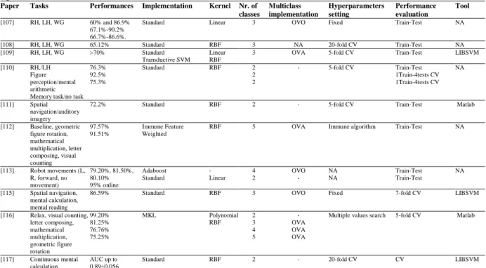
Table 3 shows the SVM features relative to motor and non-motor tasks-based BCI systems, with second column reporting performed tasks.

Table 3: SVM features in motor-non motor tasks based SMR-BCI. R= Right, L= Left, H= Hand, WG= word generation. NA= Not Available.

Paper Tasks Performances Implementation Kernel Nr. of classes Multiclass implementation Hyperparameters setting Performance evaluation Tool [107] RH, LH, WG 60% and 86.9% 67.1%-90.2% 66.7%-86.6%.

Standard Linear 3 OVO Fixed Train-Test NA

[108] RH, LH, WG 65.12% Standard RBF 3 NA 20-fold CV Train-Test NA

[109] RH, LH, WG >70% Standard

Transductive SVM

Linear RBF

3 OVA 5-fold CV Train-Test LIBSVM

[110] RH,/LH Figure perception/mental arithmetic Memory task/no task

76.3% 92.5% 75.3% Standard RBF 2 2 2 - 5-fold CV Train-Test 1Train-4tests CV 1Train-4tests CV NA [111] Spatial navigation/auditory imagery

72.2% Standard RBF 2 - 5-fold CV Train-Test Matlab

[112] Baseline, geometric figure rotation, mathematical multiplication, letter composing, visual counting 97.57% 91.51% Immune Feature Weighted

RBF 5 OVA Immune algorithm Train-Test NA

[113] Robot movements (L, R, forward, no movement) 79.20%, 81.50%, 80.10% 95% online Adaboost Standard - Linear 4 2 OVO - NA NA Train-Test Train-Test NA [115] Spatial navigation, mental calculation, mental reading

86.59% Standard RBF 3 OVO Fixed 7-fold CV LIBSVM

[116] Relax, visual counting, letter composing, mathematical multiplication, geometric figure rotation 99.20% 81.25% 76.76% 75.25% MKL Polynomial RBF 2 3 4 5 - OVA OVA OVA

Multiple values search 5-fold CV Matlab

[117] Continuous mental calculation

AUC up to 0.89±0.056

Standard RBF 2 - 20-fold CV CV LIBSVM

According to table 3, SVM with RFB kernel results to be the most adopted and accurate configuration when dealing with both motor and non-motor tasks. Different implementations are tested, even if the standard one is still the most used. CV is often adopted for hyperparameters setting, while train-test is usually considered for performance evaluation. Again, LIBSVM is widely used, even if the information about the tool is frequently omitted.

3.3.3. Other tasks

Imagery tasks different from the classical ones were used in [118], where the imagery of the “yes” and “no” words was discriminated by means of an RBF-SVM with accuracy higher than 70%. In [119] authors designed a protocol based on the imagination of two Chinese characters and used RBF-SVM to discriminate them with high accuracy (from 73.65% to 95.76%). In [120] a three-layer scheme for emotion recognition in single-trial EEG was proposed. Emotion-inductive pictures were used and valence and arousal were classified by means of imbalanced (quasi-conformal) SVM with RBF kernel. Results showed that the proposed scheme could achieve the highest classification accuracy of valence

(82.68%) and arousal (84.79%) when compared to k-Nearest Neighbors (kNN) or standard SVM. In [121] a real-time algorithm for the classification of EEG-based self-induced emotions (disgust and relax) was proposed. RBF-SVM was used for classification, achieving average accuracy higher than 90%. In [122] authors proposed a method for the recognition of implicit human intentions for developing an interactive web service engine. Brain state changes associated to navigational and informational intention were measured by using EEG phase synchrony values in different frequency bands as features. Different classifiers were compared: SVM with RBF and polynomial kernels, Gaussian Mixture Models (GMM) and Naïve Bayes. Classification accuracy was the highest for RBF-SVM: for example, for one subject, accuracy with RBF-SVM was 77.4% whereas with polynomial-SVM, Naive Bayesian and GMM it was 72.4%, 52.2% and 50.5%. The same trend was observed in all subjects.

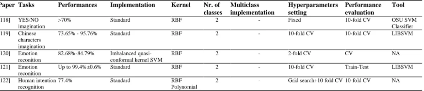
In Table 4 SVM features relative to the “other tasks”-based BCIs are listed.

Table 4: SVM features in other tasks based SMR-BCI. NA= Not Available.

Paper Tasks Performances Implementation Kernel Nr. of classes Multiclass implementation Hyperparameters setting Performance evaluation Tool [118] YES/NO imagination

>70% Standard RBF 2 - Fixed 10-fold CV OSU SVM

Classifier [119] Chinese

characters imagination

73.65% - 95.76% Standard RBF 2 - 10-fold CV 10-fold CV LIBSVM

[120] Emotion reconition 82.68%-84.79% Imbalanced quasi-conformal kernel SVM RBF 2 - 2-fold CV CV NA [121] Emotion reconition

Up to 99.4%±0.6% Standard RBF 2 - 10-fold CV Train-Test LIBSVM

[122] Human intention recognition

77.4% Standard RBF

Polynomial

2 - Grid search+10 fold CV 10-fold CV NA

RBF-SVM in its standard configuration is widely used for the classification of unconventional imagery tasks, with high accuracy. CV is widely used both for hyperparameters setting and for performance evaluation.

3.4. Steady states Visual Evoked Potentials (SSVEPs) and Slow Cortical Potentials (SCPs)

For the classification of SCPs, Qin et al. [123] proposed a semi-supervised SVM aiming at reducing the time-consuming training process. The method consisted in using both a small labeled dataset and a large unlabeled dataset to train the classifier and in implementing a batch-mode incremental training to iteratively improve the training performances. A 1-norm linear SVM further decreased training time. The method was validated with data from an EEG-based cursor control experiment and CSP was adopted for data filtering. The proposed semi-supervised SVM increased the accuracy by more than 14% with respect to a standard SVM. Moreover, the accuracy reduced by 3.25% when the standard SVM was trained with all the data (labeled plus unlabeled), but a decrease in CPU time was achieved. In [124] a method to improve BCI accuracy was proposed, based on polynomial fitting of training data and the use of a very simple kNN. This was made to discriminate brain potentials generated when moving a cursor up and down on the screen. An RBF-SVM and an ANN were also compared to the simple kNN. The latter outperformed both SVM and ANN in terms of accuracy and speed. In [125] an automated feature selection strategy, based on a decision tree, was implemented. Subjects were asked to move a cursor up and down on a screen and their SCPs were classified by means of a sigmoidal-kernel SVM, which performed with an average accuracy of 89.12%. This result was by 0.9% higher than the one obtained with an optimal electrode recombination method for feature extraction.

For SSVEPs classification, instead, in [68] authors developed a prototype of BCI-controlled wheelchair. SSVEPs elicited by four different flickering frequencies were used to control the movement of the wheelchair in four directions. Four colors (green, red, blue and violet) were used for the stimuli to investigate the influence of colors on SSVEPs. Two ANNs and an SVM were used as classifiers; different kernels were tested (order 4th _{order-polynomial, quadratic, linear) in order to select the most}

accurate one. On the basis of the results, when using violet stimuli, SVM achieved the best accuracy (between 75 and 100%).

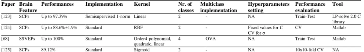
Table 5 reports SVM features relative to SCPs and SSVEPs-based BCI systems. In particular, the second column lists the exploited brain feature (SCPs or SSVEPs).

Table 5: SVM features in SSVEP/SCP based SMR-BCI. NA= Not Available.

Paper Brain Feature

Performances Implementation Kernel Nr. of classes Multiclass implementation Hyperparameters setting Performance evaluation Tool

[123] SCPs Up to 97.39% Semisupervised 1-norm Linear 2 - NA Train-Test LP-solve 2.0 C

library

[124] SCPs Up to 88.6%±1.9% Standard RBF 2 - Fixed values for C

CV for σ

CV Matlab

[68] SSVEPs Up to 100% Standard Order4-polynomial, quadratic, linear

4 OVA NA Train-Test Matlab

[125] SCPs 89.12% Standard Sigmoid 2 - NA 10x10-fold CV NA

From table 5 it is evident that different kernels are used to set a standard SVM in order to classify SSVEPs and SCPs, with almost perfect accuracy. The information about the hyperparameters setting is often missing.

3.5. Some Statistics

Figure 7 represents the percent occurrence of SVM features related to papers focused on BCI and here reviewed. The standard C-SVM implementation and the RBF kernel result as the most popular. Moreover, when dealing with multiclass problems, the OVA approach is preferred. Concerning hyperparameters setting, the CV is the most frequent method, whereas the performance evaluation adopts a train-test approach in most of the cases. Among tools, LIBSVM results the mostly utilized one. However, it is important to stress that, despite the easy accessibility of all the information regarding SVM algorithms, 20% of the available papers (not reported here) did not described the kernel type, even if its choice dramatically affects the final results. Moreover, in most of the reviewed papers, the multiclass implementation and the hyperparameters setting methodology are not described, thus leading to only partially reproducible results.

4. EMG-based HCI and SVM

4.1. Overview of EMG-based HCI systems

Surface EMG (sEMG) signals are the result of the capture of the electrical activity of muscles, recorded on skin surface. Similarly to BCI systems, sEMG-based HCIs found their major applications in the field of assistive devices and rehabilitation. They have been mainly exploited to control multifunction prostheses of the upper limb [126] or the lower one [127]; to drive electric power wheelchairs [128]; to recognize facial gestures [129]; to control a mobile robot [130] or a manipulator system [131]; to

Figure 7: Percent occurrence of the different SVM features (Implementation, Kernel, Multiclass Implementation, Hyperparameters setting, Performance evaluation, Tool). Values are obtained from literature works regarding EEG-based HCIs. LS= Least-Squares; sw= Spatially-weighted; RVM= Relevance Vector Machine; MKL= Multiple Kernel Learning; RBF= Radial Basis Function; DAG= Directed Acyclic Graph; CV= Cross Validation; GA= Genetic Algorithm; PSO= Particle Swarm Optimization; LOO= Leave-One-Out; NA= Not Available.