Improving credit scoring by differentiating default behaviour

Improving credit scoring by differentiating defaulter

behaviour

Cristián Bravo1,3*, Lyn C Thomas2and Richard Weber3

1_{Departamento de Modelamiento y Gestión Industrial, Universidad de Talca, Curicó, Chile;}2_Southampton School of Management, University of Southampton. Highfield, Southampton, UK; and3Department of Industrial Engineering, Universidad de Chile, Santiago, Chile

We present a methodology for improving credit scoring models by distinguishing two forms of rational behaviour of loan defaulters. It is common knowledge among practitioners that there are two types of defaulters, those who do not pay because of cashflow problems (‘Can’t Pay’), and those that do not pay because of lack of willingness to pay (‘Won’t Pay’). This work proposes to differentiate them using a game theory model that describes their beha-viour. This separation of behaviours is represented by a set of constraints that form part of a semi-supervised constrained clustering algorithm, constructing a new target variable summarizing relevant future information. Within this approach the results of several supervised models are benchmarked, in which the models deliver the probability of belonging to one of these three new classes (good payers,‘Can’t Pays’, and‘Won’t Pays’). The process improves classification accuracy significantly, and delivers strong insights regarding the behaviour of defaulters.

Journal of the Operational Research Societyadvance online publication, 7 May 2014; doi:10.1057/jors.2014.50 Keywords:credit scoring; statistics; domain-knowledge; constrained clustering; banking; game theory

Introduction

Credit scoring (Thomas et al, 2002) is one of the most widely known applications of statistical models and data mining, whose goal is to differentiate between customers who will pay back a given loan, and those who will not. Classifying borrowers into these two groups (defaulters and non-defaulters) has been the standard approach of credit scoring from its inception. Lately, there has been a rise in the number of statistical models that use economic analysis and game theory to better understand the behaviour of the relevant players in many applications. It has been used to improve manufacturing strategies (Wang, 2007), in credit card fraud detection (Vatsaet al, 2005), and inphishing

detection for spam filtering (L’Huillieret al, 2009), to name a few. In this paper, we present a procedure that extends applica-tion credit scorecards by differentiating defaulters into two groups, those who default due to the lack of willingness to repay, and those who fail to pay because they do not have the capacity to do so.

The relationship between lenders and their borrowers has been studied by a number of authors modelling who are defaulters and what are the probabilities of default. For example in the well-known work of Stiglitz and Weiss (1981), the authors imposed conditions on the rationality of the players, which produce an adverse selection game in the credit granting process. The

importance of collateral as a way of selecting customers was also studied by Wette (1983). Both papers point out that the drivers for the decisions of whether to request a loan and whether to grant the request include the amount of the loan and the collateral offered.

More recent works have focused more on reasons and characteristics of default. Alary and Gollier (2004), using collateral and amount lent as their main decision variables, emphasized the moral hazard problem that lenders faced, and showed that under certain conditions customers will default strategically. Moffat (2005) used hurdle models to model default, and the extent of it, also finding different levels or intensities of default. Block-Lieb and Janger (2006) suggested that the expectation that borrowers will be fully rational is not true in some cases, and that it is not reasonable to assume that

all customers behave strategically. The work of Guiso et al

(2010) also focused on the reasons that drive default, and found that there are segments of the population that default strategi-cally, and that such behaviour is driven by economic and moral variables. Finally, differences in default and the characteristics of defaulters have also been studied in small business lending, with Linet al(2011) defining four different types of default depending on thefinancial conditions of borrowers.

The literature agrees that there are different reasons for defaulting, even though credit scoring aggregates these different reasons into just one default class, which is normally defined as being 90 days in arrears (Thomas, 2000). Then one usually estimates the risk of this happening in the next year. Our *Correspondence: Cristián Bravo, Department of Modelling and Industrial

Management, Universidad de Talca. Camino a Los Niches Km. 1, Curicó, 3344158, Chile.

proposal is to differentiate between two types of default, for both willingness and capacity to repay, by usingfirst economic modelling, and then semi-supervised clustering. Then it is possible to build a scoring system using supervised techniques such as logistic regression or neural networks to predict whether a borrower will default for each specific reason.

This paper is divided as follows: The next section presents a game theory model that determines which combination of collateral, loan rate charged, and borrower/lender characteristics lead to loans being given, but then defaulted upon. The borrowers are assumed to belong to one of two groups; those who are unwilling to repay the loan (colloquially referred to as

‘Won’t Pays’) and those who want to repay but may default because they do not have the capacity to repay (colloquially called‘Can’t Pays’).

The subsequent part of the paper shows how the behaviours described by the economic model can be used as input for a semi-supervised clustering procedure, which separates bor-rowers into one of the two classes. In order to demonstrate the usefulness of the proposed model, the resulting procedure is

applied to a dataset of actual loans in the ‘Validation and

experimental results’section. In it, the clustering procedure is conducted to find which are the ‘Won’t Pay’ and which the

‘Can’t Pay’ clusters. Then, two supervised learning models (neural networks and multinomial logistic regression) are used on the data using the cluster labels as targets. The results of the supervised models are benchmarked against the classical logistic regression model based on the whole, un-clustered, population to obtain an overall estimation of the borrowers’ credit risk, focusing on both the gains in accuracy and the knowledge obtained. Finally, the conclusions extracted from building such a model are outlined.

Game theory model of the loan granting process

Throughout this paper we will assume there is a set of N

borrowers that were granted a loan. Each loan is described by a set V of different variables, stored in database XRjVj;

representing the different characteristics of the loan, the bor-rower, and the evolution of the loan. There is also an outcome variable, given by di∈{0, 1}, associated with each xi∈X (i∈{1,…,N}), indicating whether borroweridefaulted on that loan or not. Only the characteristics inV,which describe data known before the loan was granted, can be used for classifi ca-tion, which we denote asVpast⊂V, forming a datasetXpast. The remaining characteristics,Vfuture=V\Vpastand the correspond-ing datasetXfuture, consist of information that can only be used for determining whether and for what reasons the borrower has defaulted. The database will consist of different applicants, with one loan per applicant, as is common in application scoring.

In general, a game is defined by its players, their strategiessi, and the payoffsui(si,s−i) of playing the various strategies in the competitive or adversarial setting (Fudenberg and Tirole, 1991), wheres₋irepresents the strategies played by all other players

excepti. In the model of the loan granting process presented in

this work, the first player, L, is the lender who wants to

maximize the profit of lending toNpotential borrowers over two time periods.

The borrowers can be of two types,CorW, whereCs are

the‘Can’t Pays’who are willing to pay back the loan they received provided they are able, and so will only default because of the occurrence of an external shock that can occur with probabilityq, that can be, for example, job loss of

the borrower. Considering that we will perform classifi

ca-tion further on, we will refer to the types of borrowers as either types or classes. ClassWcorresponds to the ‘Won’t

Pays’who are unwilling to pay back the loan even if they

can afford to do so, and so presumably took the loan with no intention of paying it back. We can also identify the good payers (classP) as members of classCthat are not subject to an external shock, and thus were able to repay the loan.

The mechanism for granting loans will be the following: in thefirst period borroweri∈{1,…,N} can ask for a loanai1, and the lender can agree to or refuse this request, whereyi1=1 is accepting the loan request andyi1=0 is refusing it. The loan is paid at the next period together with the interest, at an interest rate of r, charged on the loan. The lender could also ask for collateralCi1from the borrowerito secure the loan, whereCi1 could be, for example, the deed to the house on which a mortgage is taken out; or the lender could grant the loan without collateral (an unsecured loan, ieCi1=0). If the loan is not repaid, the lender will sell the collateral but will only get an amountαCi1 back, withα∈[0, 1], so (1−α) is the so-called‘haircut’on the collateral. Borrowers of typeCwill not be able to repay if they

have had a shock to their cash flow during the period, while

those of typeWwill not pay no matter what their cashflow is. We assume that a shock leads to default, and if no shock

occurs then borrowers from classCwill always repay. On the

basis of this assumption we can focus our analysis of the decision process just on the marginal income that the loan brings to the borrowers. Our assumption occurs in segments in which income is concentrated in a narrow range, a common occurrence for micro-entrepreneurs and low-income consu-mers, as we will show in the experimental section below.

If the loan is repaid, the borrower can repeat the process in the second period asking for a loan of valueai2which, if it is given, will correspond to decisionyi2=1 by the lender, as opposed to

yi2=0 if refused. The interest rate remainsr, but the collateral this time would beCi2. If the loan is not repaid in thefirst period, the borrower will not be granted a new loan in the second period. If thefirst loan was not granted, it is not reasonable that this would be different in the second period, so it will not be granted as well. The time dependence of the players’utility is given by discount rates defined to beδL,δC, andδWfor the lender and the two types of borrowers, respectively.

If we do not restrict the total amount of money that the lender has available, then this procedure can be considered as a series of two-player games between the lender and each of the individual borrowers. In this case, without loss of notation, we

will ignore the indexiof each borrower. The payoff of the two types of borrowers and the lender,uC,uW, anduL, will depend on the strategiess=(y1,y2,aC1,aC2,aW1) chosen, together with the a priori probability that the borrower is in class C, represented byθ∈(0, 1). The lender does not know which type the current borrower is. This is private information that the borrower has, so this is a game with incomplete information.

The expected utility of the borrowers is the net present value of the loans they receive, according to their type:

uCð Þ ¼s y1ðaC1-qδCC1-ð1-qÞδCð1+rÞaC1Þ

+ð1-qÞδCy1y2ðaC2-qδCC2

-ð1-qÞδCð1+rÞaC2Þ ð1Þ

uWð Þ ¼s y1aW1-y1δWC1 (2)

The utility of the lender is the expected value of the returns from the loans:

uLðsÞ ¼y1ð1-θÞð-aW1+δLαC1Þ

+y1θð-aC1+qδLαC1+ð1-qÞδLð1+rÞaC1Þ

+θð1-qÞδLy1y2ð-aC2+qδLαC2

+ð1-qÞδLð1+rÞaC2Þ ð3Þ

To derive the set of conditions that the player must satisfy, we will create a set of constraints that account for the individual rationality of the players given what was observed to occur, that is, we will demand that the best possible choice is to request and grant the requested loans.

We will assume one condition for this setting: that the strategy of granting or requesting two loans (or one in case of borrowers in classW) is individually rational. Thus, requesting and granting two loans has a higher utility compared with not participating or to just requesting a loan in one period for class

C, which would bring a marginal utility equal to zero. For the lender, the conditions are:

uL 1;1;C1;C2;s0_-i ⩾uL 1;0;C1;0;s0_-i 8C1;C2 (4) uL 1;1;C1;C2;s0_-i ⩾uL 0;0;0;0;s0_-i 8C1;C2 (5)

The right-hand side (RHS) of (4) is equal to:

uL 1;0;C1;C2;s0_-i

_¼

θaC1ð-1+δLð1-qÞð1+rÞÞ

-ð1-θÞaW1+δLαC1ð1-θ+θqÞ ð6Þ

And so (4) is equivalent to:

aC2ð-1+δLð1-qÞð1+rÞÞ+ð1-qÞqδLαC2⩾0 (7)

(5) is equivalent to:

θðaC1+aC2δLð1-qÞÞð-1+δLð1-qÞð1+rÞÞ

-ð1-θÞaW1+C1αδLð1-θð1-qÞÞ

+θð1-qÞqδ_L2αC2⩾0 ð8Þ

To obtain the solution space, the same analysis has to be carried out for each borrower. For borrowers of classC, the inequalities that must be satisfied are:

uC aC1;aC2;s0_-i ⩾uC aC1;0;s0_-i (9) uC aC1;aC2;s0_-i ⩾uC 0;0;s0_-i (10) Note that this assumes thaty1=1 andy2=1, that is inequal-ities (4) and (5) are satisfied. This is reasonable because every other decision implies utilities ofuC(0, 0,s′−i), that is, no loans are granted.

The RHS value from (10) equals zero, so the borrower only asks for a loan if she or he receives positive utility. Incorporat-ing that into (10) implies:

aC1ð1-δCð1-qÞð1+rÞÞ

+δCaC2ð1-qÞð1-δCð1-qÞð1+rÞÞ

-δCqC1-δ2Cð1-qÞqC2⩾0 ð11Þ

Condition (9) assumes that the expected utility that arises from applying for a second loan must be positive, so that:

aC2⩾ δ

Cq

1-δCð1-qÞð1+rÞ

C2 (12)

Finally, borrowers of classWwill apply for a loan if their respective utility is greater than the discounted collateral they would lose if they received the loan:

aW1⩾δWC1 (13)

The set of inequalities (7), (8), (11), (12), and (13) creates a behaviour space. This set of inequalities can be interpreted as a set of constraints that will be used to separate the behaviour of the defaulters. A defaulter of classCdesires a second loan even though this will be refused since he or she will have defaulted,

while a defaulter of class W does not expect a second loan.

Given this set of constraints, it is now possible to actually differentiate the defaulters: we can obtain two groups, each one with cases that are similar (in variance) and that satisfy the proposed constraints.

Some other interesting results that arise from the proposed model are as follows:

● _{Since the left-hand side (LHS) of (5) is increasing inC1,C2,} andδLthe collaterals are an incentive for the lender to grant loans. Similarly, a lower expected return on capital, and so a higher discount factorδL, increases the chance the loan will be given.

● _{(12) and (13) show that borrowers might accept a loan even if} the collateral demanded is of greater value than the loan itself. Such event is observed in real life, for example, when a loan tofinance a percentage of a car is secured by the value of the car in full.

● A necessary condition for the set defined by the constraints to be non-empty is thatδW<δC<δL. This is reasonable since people who need to borrow have lower discount factors than

assumed to be more short-sighted than the other types of borrowers. A high value ofδWwould also result in that group being limited to very high loan amounts (relative to the collateral), or to borrowers with no collateral.

We propose a learning model that incorporates such restrictions in the next section.

Constrained clustering and semi-supervised methods

Constrained clustering (Basuet al, 2008) is a semi-supervised approach to obtaining segments of a dataset incorporating certain restrictions that must be fulfilled by the members of the cluster, the members of different clusters, or the general structure of the clusters. The term ‘semi-supervised’refers to the incorporation of knowledge that is not directly present in the data—or that is known only for a limited number of cases—in order to improve the results on the whole domain. In this particular case, restrictions are added to a clustering procedure so that the objective is not only to minimize intra-cluster variance, but also to satisfy a set of conditions for each member, or each cluster. The methodology has been applied successfully

in several fields, ranging from signal processing (Levy and

Sandler, 2008), epidemiology (Patil et al, 2006), to OR

applications (Bard and Jarrah, 2009).

There are two different approaches for constrained clustering, as noted by Davidson and Ravi (2005), and both are based on the concept of‘Must-Link’and‘Cannot-Link’constraints. The

first set of restrictions indicate that two elements must be in the same cluster, whereas the second set prohibits the presence of two elements in the same cluster. The methods differ in the role of restrictions: in the first case the algorithm satisfies an objective or distance function using the information from the constraints. The best-known application of this work is by Basu

et al(2004). In the second case the constraints simply limit the presence of elements in the same cluster. Our work uses the second approach, with an adjustment that adds some complex-ity: the elements in one cluster must satisfy the restrictions against most of the elements of the other cluster. There are algorithms that solve this particular problem, such as the Constrained Clustering with Filtering (CCF) algorithm intro-duced by Bravo and Weber (2011), which will be used in this paper.

A constrained clustering model to differentiate defaulters

The constraints obtained from the economic assumptions from previous sections can now be used to design a new objective variable using semi-supervised methods. The overview of the process is as follows:

1. Select defaulters from the database X, and describe them

using only the information inXfuture, composed of variables inVfuture, that is, variables collected after the loan has been granted.

2. Cluster elements into two groups, one for each type of defaulter (CandW) using the CCF algorithm with dataset

Xfuture as input. The constraints defined in the previous section are extended now to the whole cluster, requiring that most cases in the cluster assigned to classWhave to satisfy their own condition, Equation (13), and that elements in the cluster assigned to classCmust satisfy constraints (7) and (10). Finally there is a cross-cluster constraint, given by the lender condition (8), which must be satisfied by‘most’pairs of elements in different clusters.

3. With the elements clustered, the new objective variable extends the default variable to the new case when there are three different cases: good payers, defaulters in classC, and defaulters in classW.

The exact constrained clustering problem to be solved considers two groups with centroids given byck,k={1, 2} and a binary variablemifor eachi∈{1,…,N} that represents the class of the borrower (1 for classC, 0 for classW). Since the value of the second loan and the second collateral are not known, we will assume they are a fraction of the original value requested (fCr andfCol), as explained below. Since now each borrower has his or her own variables, we will refer to the amount borrowed as

ai∈xi, to the collateral given for thefirst loan as Ci∈xi and finally to the interest rate paid asri∈xi, withxithe vector of variables for each borrower/loan.

The problem is then to solve the following optimization problem, adapted from the formulation presented by Dogan and Guzelis (2006): min m1;m2;c1;c2;maxW;minC XN i¼1 mikxi-c1k2+ð1-miÞkxi-c2k2 ð14Þ s:t: minC⩾ð1-θÞai 8i j mi¼0 xi⩾δWCi 8i j mi¼0 0⩽aið1-δCð1-qÞð1+riÞÞ ´ð1+δCfCrð1-qÞÞ -CiδCqð1+δCfCoÞ 8i j mi¼1 0⩾θaið-1+δLð1-qÞð1+riÞÞ ´ð1+fCrδLð1-qÞÞ +CiαδLð1-θð1-qÞqδLfCoÞ -ð1-θÞmaxW 8i j mi¼1 minC⩽θaið-1+δLð1-qÞð1+rÞÞ ´ð1+δLfCrð1-qÞÞ +CiαδLð1-θð1-qÞ +θfColð1-qÞqδLÞ 8i j mi¼1

maxW⩾ai 8i j mi¼0 c1¼ PN i¼1mixi PN i¼1mi c2¼ PN i¼1ð1-miÞxi N-PN_i¼1mi mi2 f0;1g 8i2 f1;¼;Ng ð15Þ

Expression (14) represents a quadratic objective function with integer variables. The constraints (15) depend directly on the cluster in which the elements are present, so an extensive expression (one that does not include themiparameters in the description) would have to includeN2constraints, one for each pair of elements, turning the problem intractable for large databases.

The CCF algorithm follows a similar methodology as the K-Means algorithm, extending the procedure for constrained problems. In each iteration the set of constraints for each element is checked, that is, if the element is in class C, then Equations (11) and (12) are evaluated for the element itself, and Equation (8) is evaluated against the extreme values arising from the elements currently in the cluster assigned to classW. In case the conditions are not fulfilled, the element is moved from its original cluster, and if that does not solve the issue, the elements with extreme values in both clusters are removed from the analysis and the process is repeated. The algorithm continues until the violations are below a threshold and the centroid values do not move more than a given tolerance.

The elimination of cases with extreme values in each iteration relaxes the problem. The elements in each cluster have to satisfy the constraints against most of the elements in the other cluster, and this is accomplished by eliminating a small number of extreme cases in each iteration and ensuring that all remaining cases satisfy the constraints. In the end, since the

final cluster for each element is determined only by proximity to centroidsc1andc2, it is possible to re-assign even the cases that were eliminated from the clustering procedure.

One of the open questions that remain is what are the possible values of the parameters required to estimate the model. We propose the following values, which correspond to realistic measures in credit risk:

● θ: This parameter represents the a priori probability of a customer being in the class ‘Can’t Pay’. The lender can estimate this value from historical data, using two different approaches: In the experimental part of this paper the proportion of defaulters among all defaulters that made a payment until up to 2 years after the default occurred was

used as an approximation of θ. This is based on the

assumption that defaulters of typeWpay back very little of the loan or nothing at all. The second method is using the number of instalments paid, since defaulters in classWare

expected to repay very little, if nothing at all, of the loan. In this case the proportion of borrowers who default in thefirst instalments of the loan are an approximation of the value

1−θ. Note that this value would have to be adjusted to

account for borrowers in classCthat suffer a liquidity shock in thefirst few months.

● _{q: This parameter represents the chance that a borrower}

receives a shock to his or her income, and so is forced to default. This value could correspond to the long-term default rate for loans, because it is expected that in the long term, most of the‘Won’t Pay’borrowers arefiltered from the database. Another option (and the one used in the experimental results section) is to discount the observed

default rate (DR) by a small amount, in order to include

the unobserved segment. A possible value would be

q=(DR⋅(1−θ)/2).

● α: The expected recovery to be extracted from the collaterals is a known value to credit granters, with values commonly between 40% and 60% of the collateral value (see for example Yamashita and Yoshiba, 2010 or Jokivuolle and Peura, 2000).

● _{δL: The value of the discount factor for a company should be} a known value, for example if the expected internal return rate for the fiscal year is τ, then the company’s discount factor would be 1/(1 +τ).

● _{δCandδW: The value of the discount factor for the customers} is more difficult to determine. Individual discount factors have been studied on several occasions with widely different results. For example Burkset al(2008), Chabriset al(2008), and Greenet al(1994) report discount rates ranging from 0.1 to 0.9 depending on several factors, although these studies do

not focus on financial decisions. The well-known paper of

Benzionet al(1989) gives discount factors depending on the

financial amount at risk that ranges from 0.2 to 0.75, with a strong dependence on both the amount at risk and the duration of the loan. We can imply from such studies that there is a time-value of money, which allows lending money to occur, but that the exact value of such discount factor is hard to measure. We propose an exogenous measure, which limits the range of choices that a borrower has for such rate. In many countries there is a legal limit for the annual rate that can be charged by lenders, and this limit can be justified as a constraint on an irrational behaviour from the borrowers facing an extreme situation. Low tomiddle-income borrowers intuitively understand these limits and make rational deci-sions without them (Littwin, 2007). The maximum interest rate allowed for loans, which represents the maximum discount rate that any customer is legally bound to pay, can then be a good proxy of the maximum rate a rational borrower would accept. We proceed with the modelling processfixing that value forδC. As forδW, the value has to

be lower than that associated with customers of class C,

because their demand for the loan is more immediate. We study a range of values in [0,δC] in the ‘Validation and experimental results’section.

● Values for the second loan: Two of the parameters that must be decided are the values for the second loan and the second collateral. Since defaulters were not allowed to take a new loan, these values are unknown, but they are known for the customers who successfully paid back their loans. Good proxies for these values are the proportions between the amounts that were requested/granted by returning borrowers, that is, the average value offCr= (Second_Amount/First_-Amount) andfCol=(Second_Collateral/First_Collateral) cal-culated for borrowers who successfully returned granted loans and received new ones.

Validation and experimental results

In this section we present the results of applying the proposed approach to a dataset of loans granted at afinancial institution. First the dataset is introduced, then we present the procedure of constrained clustering on the defaulters from this dataset. In the section‘Sensitivity analysis and parameter selection’we perform those analyses. Finally, we discuss in detail the obtained results.

Available dataset

A dataset consisting of 97 254 loans granted to mass-market, low to middle-income independent borrowers (with a monthly income ranging from USD 300 to USD 2000) was used. The database originates from a Chilean public organization, and comprises an 11-year period, from 1997 to 2007. The dataset has a default rate of 25.2%, with each loan described by 25 different variables. One of the main characteristics of the dataset is that the organization almost never rejected a loan: its reject rate was just 2%, so there is little need to use reject inference. This extremely low rejection rate also explains the very high default rate, as will be reflected in the composition of the cases in classesCandW.

The variables available for classification, that is the ones obtained before granting loans are as follows:

● _{Economic activity: The sector of the economy in which the}

customer is involved (through his/her job or company). The large number of sectors was clustered to improve interpreta-tion of the variable, mapping the 47 different sectors to three larger groups (Activity_A, Activity_B, and Activity_C), and the last one was selected as a reference category.

● Ownership of housing: This shows if the customers own, rent, or hold other types of agreements on their current home. Four classes are recognized: Owner, Tenant, Share-Tenant (Share), or other types. The class‘Others’is used as a reference.

● _{Number of properties: The number of properties the}

bor-rower possesses. The variable was divided into three cate-gories: No properties, one property, or two or more properties, which was used as a reference category.

● _{Region of country: Division of the country into three regions,} one of them (arbitrary) used as a reference.

● With guarantor: Whether the customer has a guarantor for the loan or not.

● Length of loan: The length of the loan requested by the

borrower. This number is determined by the customer, with the company simply granting the loan or refusing it, so it is not susceptible to manipulation. The durations of the loans are between 1 and 12 months.

● _{Age: The age of the customer in years.}

The previously presented variables describe the customer at the moment of requesting the loan. On the other side, the variables that describe the actual evolution of the loan are as follows:

● Collaterals: The collaterals are described by two variables.

The first is a dummy variable that describes whether the

customer had to give collateral on the loan (With_Collat-erals), and the value of the collateral (Value_Collateral_UF).

The latter is given in ‘development units’ (Unidades de

Fomento, referred to as UF for their acronym in Spanish), the Chilean inflation-indexed unit, that is equivalent to roughly 46 USD.

● _{Amount and rate: The amount of the loan, in UF, and the}

total annual interest rate charged for the loan.

● _{Days in arrears before defaulting (Days_Arrear): The total}

number of days the instalments of the loan were in arrears before defaulting. For example, if a loan defaulted in the fourth instalment, and the first was paid 10 days late, the second on time, and the third 45 days late, the variable has a value of 55.

● Cancellations: Sometimes the institution will cancel the

payment of penalties and excess interest that arises from arrears, upon agreement that the next instalment is paid on time, or that a renegotiation is performed. This event is summarized into two different variables, considering the number of times this happened in the lifetime of the loan (Num_Cond), and the amount that was reduced (Amount_-Cond). In addition, if some of the interest due to be paid is also discounted from the instalments, this value is reported in the variable Interest_Low.

● _{Extensions: Sometimes the company will extend the period}

of an instalment for 30 days or a similar span of time, subject to adjustment in the amount owed. The number of times a customer applies for this appears in variable Num_Post, and the amount adjusted appears in Amount_Adjust, and, since the adjustment can be positive or negative, the total amount of negative adjustments is incorporated into Negative_Adj.

Clustering procedure

For the clustering procedure, the parameters used, their values, and their origin are shown in Table 1.

The process is run using the 24 576 customers flagged

as defaulters, normalizing the dataset with all the future variables. The results consist of two clusters, each one

corresponding with a class, eitherCorW. In thefirst cluster

there are 4762 borrowers, which are assigned to Class C,

while the second cluster has 19 814 borrowers, which are

assigned to classW. The centroids for each class are shown

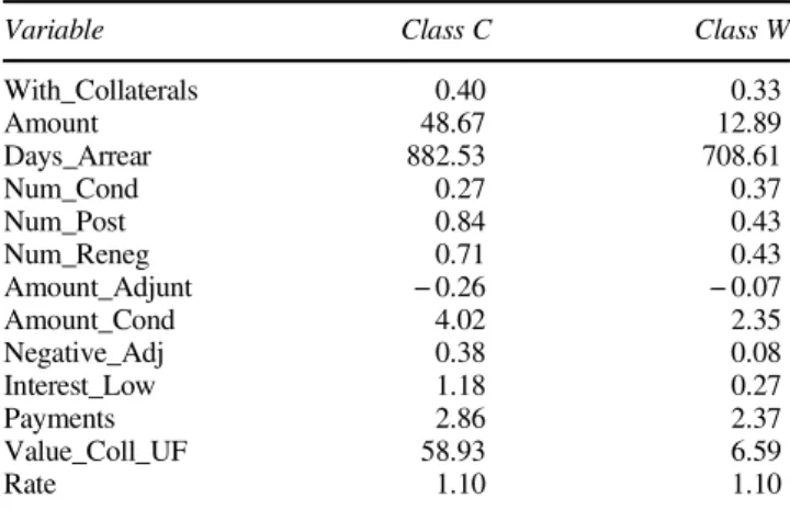
in Table 2. The variables associated with collaterals have a greater impact in differentiating the clusters, even though the difference in the percentage of customers with collaterals

is not huge (40%versus33%). The value of the collaterals

for classCis almost nine times greater than that in classW. Since the percentage of borrowers with collaterals are relatively balanced between the two clusters, this result shows that it is not whether a loan is secured or not what differentiate defaulters, but what the value of the collateral is, which is an interesting result.

Customers in classC request a far larger amount for their

loans, which would be consistent with a default based on the capacity to repay. Considering the total number of days in arrears, classCaccumulates almost 100 days more than classW

before defaulting, indicating that they make a greater effort to

pay back the loans than customers in class Wdo. Also, they

apply for a larger number of renegotiations (0.71 per customer on average), get greater adjustments and debt relieves, and are more susceptible to receive a discount on their interests due (1.18 UF per customer on average,versus0.27). The values of the variables suggest that there are, indeed, different behaviours detected.

Sensitivity analysis and parameter selection

In order to analyse the sensitivity of the clustering parameters, the procedure was run using several values of the parameters (δW,α). The value of δW was tested in the range [0, 0.6], following the restrictions presented in the previous section, andαwas simultaneously tested in the range [0.4, 0.6].

Para-meterαwas varied in steps of 0.05, while parameterδWwas

varied in steps of 0.1.

Table 3 presents the obtained results, and shows that when the discount factor for the‘Won’t Pays’(δW) is low, then the model assigns a large number of cases to that class. This is reasonable as a low value in the discount factor implies a more relaxed constraint, so it is easier to satisfy the restrictions for that class. Of greater interest is that this dependency presents very little variation when varying parameterα for all values

except δW=0.6, which seems to imply that after a certain

threshold, the restrictions tend to balance and more cases can be

assigned to class C. Higher values of parameter α relax the

constraints applied to classC, but this effect was not strong until the discount factorδWreached a value of 0.5.

Considering the results obtained, the values δW=0.5 and

α=0.6 are selected. This is done because the number of

elements in the cluster assigned to class W decreases for

increasing values of δWwithin the interval (0.5, 0.6). Outside this interval the respective number does not vary notably. This indicates that the value of δW=0.5 is a critical value for the discount factor. WithδWfixed at 0.5, a value ofα=0.6 presents

approximately 6600 cases in class C, which is a sufficient

number to ensure a valid statistical model when applying supervised models for classification.

Of note is the large percentage of cases assigned to classWin comparison to classC. This suggests that willingness to repay, not capacity to repay, is the most important factor that determines default for the analysed data. It is to be believed that this imbalance might be caused by three different factors:

first, since the rejection rate of the organization is extremely low, then it follows that the organization possessed poor evaluation standards previous to the implementation of a scoring system, as we know it is the case. Bravoet al(2013) evaluated the impact of implementing a scoring system for this organization. Second, the clustering methodology itself has an Table 1 Parameters selected for clustering experiment

Parameters Value Origin

q 0.130 Adjusted default rate

θ 0.550 Estimated from historical return data

α 0.600 Range [0.4, 0.6]

δL 0.935 Company factor—10% inflation

δC 0.625 55% maximum annual rate (Central Bank) δW 0.500 From sensitivity analysis

fCr 1.320 Examples from good payers

fCol 2.470 Examples from good payers

Table 2 De-normalized results of semi-supervised clustering

Variable Class C Class W

With_Collaterals 0.40 0.33 Amount 48.67 12.89 Days_Arrear 882.53 708.61 Num_Cond 0.27 0.37 Num_Post 0.84 0.43 Num_Reneg 0.71 0.43 Amount_Adjunt −0.26 −0.07 Amount_Cond 4.02 2.35 Negative_Adj 0.38 0.08 Interest_Low 1.18 0.27 Payments 2.86 2.37 Value_Coll_UF 58.93 6.59 Rate 1.10 1.10

Table 3 Percentage of cases in classWdepending on parametersα andδW δW/α 0.40 0.45 0.50 0.55 0.60 0.0 100.00% 100.00% 100.00% 100.00% 100.00% 0.1 100.00% 100.00% 100.00% 100.00% 100.00% 0.2 100.00% 100.00% 100.00% 100.00% 100.00% 0.3 86.17% 85.08% 80.14% 86.17% 81.13% 0.4 74.52% 74.09% 74.32% 75.09% 75.06% 0.5 79.82% 74.56% 72.14% 71.92% 70.79% 0.6 77.99% 78.78% 78.14% 69.51% 69.58%

impact in the imbalance of the classes, since class C has an additional constraint that might make it harder for a case to be assigned to it, but this can be easily measured by the sensibility analysis performed, as we have shown in this section. Afinal factor is that loans tend to default at a constant, higher rate, during thefirst months of repayment, as shown for example in Baesenset al(2005) and this rateflattens at thefinal stages of the loan. Such cases of early default will be assigned to classW

but are actually class C cases who have defaulted early.

Combined with the second factor this will increase the number of cases in classW.

Classification results

In order to show the potential of our proposed approach we apply two different procedures to the same dataset. First, we apply standard logistic regression without differentiating defaulters, and then we apply two methods for classification with three classes (C,W, andP), namely multinomial regression and a feed-forward neural network with a Multi-layer Percep-tron architecture.

Multinomial logistic regression (Hosmer and Lemeshow, 2000) is the natural extension of the binomial logistic regression model, which in turn is the most widely used technique for building credit scorecards, as noted by Anderson (2007);

Siddiqi (2006); Thomas et al (2002). The method uses only

two logistic regressions. The first compares classes CandW

and leads to coefficientsβCand the second comparesPandW

and leads to coefficientsβP. The classification function for each classk,k∈{P,C} is then: pkð Þ ¼x exp βk₀+PjVpastj j¼1 β k jxj 1+ P k02fP;Cg exp βk0 0 + PjVpastj j¼1 β k′ jxj (16)

and for classWthe classification function is:

pkð Þ ¼x 1 1+ P k02fP;Cg exp βk₀0+PjVpastj j¼1 β k0 jxj (17)

The second multinomial model used is feed-forward neural networks, judged to be the most accurate procedure for credit scoring according to Baesenset al(2003). Neural networks are known black-boxes, but several adjustments can be made to the design in order to obtain parameters that are consistent with probabilities and that satisfies the legal requirements that are common in credit scoring (De Waalet al, 2005). In particular, a configuration based on linear transfer functions and softmax

(logistic) output functions is used. In this case, a probability

matrix of dimension (|Vpast|+ 1) × 3 is obtained. The

classification function for eachk,k∈{P,C,W} is:

pkðxÞ ¼ exp βk₀+PjVpastj j¼1 β k jxj P l2fP;C;Wg exp βl₀+PjVpastj j¼1 β l jxj (18)

The results from both models are benchmarked against the results from a regular logistic regression, which delivers a unique set of parameters β¼ ðβ0;¼;βjVpastjÞ that construct probability p(x) of being a defaulter in class D={C,W}, a unique class. The expression ofp(x) is:

pðxÞ ¼ 1

1+exp -β₀-PjVpastj

j¼1 βjxj

(19)

In order to construct the experiments, a balanced sample was taken from databaseXpast, selecting 14 286 cases representing the three classes. Then 10-by-10 cross-validation was applied to the dataset to obtain the parameters and their deviations (Hastie

et al, 2009). For training the neural network, an additional step—extracting one of the folds of the cross-validation set to search for the optimal parameter configuration—was taken, a crucial step in order to get useful results in these types of statistical models (Zhang, 2007). Since the training is performed 100 times, a set of 100 results is obtained for both the parameters and the performances of the models. In all tables that are presented the‘mean±std. deviation’of these results is reported.

The results for the different models can be seen in Table 4. The results displayed are aggregated, that is, the obtained probabilities are transformed into defaulters and non-defaulters, which is performed by simple addition of the probabilities of default. This is done in order to facilitate comparison with the

binomial model, which differentiates between Pand D. One

could combine the scores in other ways (Zhuet al, 2001), but we believe that the direct methodology is the obvious approach in this case. This comparison also takes into account the fact that the final goal is to have a better discrimination between these two classes, defaulters and non-defaulters. The results obtained are more clearly viewed when the Area Under the Curve (AUC) is considered and the Receiver Operator Char-acteristics (ROC) curves are plotted. Table 4 shows the AUC that is obtained for each model, and Figure 1 displays the comparison between the models. The proposed methodologies obtain results that are 5–7% better than the logistic regression model. The AUC of the two models with the two types of defaulters are statistically insignificant in value, but both are superior to the logistic regression. The ROC curve also shows

Table 4 AUC for the three models

Model AUC (defaulters)

Logistic regression (w/o defaulter diff.) 0.6275±0.017 Multinomial logistic regression (w/ defaulter diff.) 0.6678±0.004 Neural networks (w/ defaulter diff.) 0.6660±0.004

that the multinomial models are better at identifying defaulters in the upper range of scores, showing a significant difference when more than 30% of the true positives have been detected. This suggests the increase can be attributed to the improvement in discriminating between the two types of defaulters. Since the dataset was obtained given a very low rejection rate, and that the increase in discrimination capacity comes from a better differentiation of defaulters, the improvement that the metho-dology brings is subject to the proportion of cases in each class

that any potential user has; a bank better at filtering bad

borrowers (class W) might not see such a large increase in

default prediction, whereas an institution with lower standards (as the one used in this example) will observe better results.

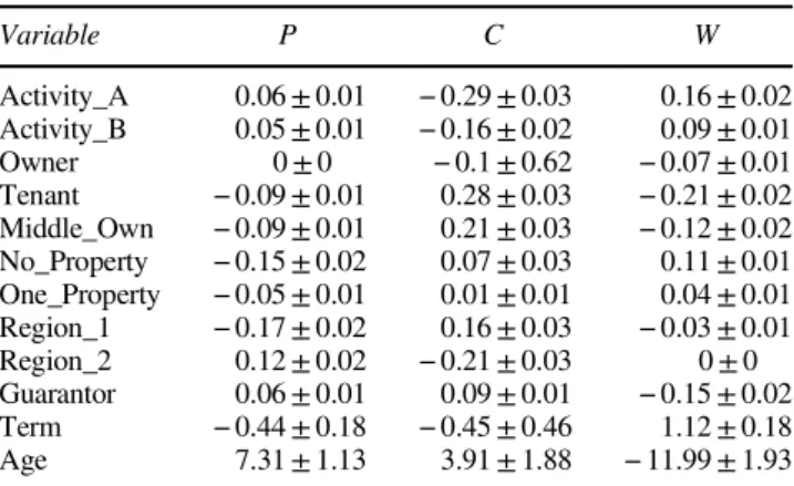
In Tables 5, 6a and 6b the parameters from the experiments

can be observed. The first conclusion that can be drawn from

the parameters is their low standard deviation, hinting to very

stable solutions. The improvement in classification can be

explained by those variables whose β parameters for good

payers lies in between the respective parameters for classesC

andWas happens, for example, with the variable‘Tenant’. This variable is not significant in the binomial logistic regression model. It is though in the other two models, with both models showing that being a tenant is a characteristic present for customers who do not have the capacity to repay, and that it is a neutral characteristic for good payers. Owning a house, in turn, is not a characteristic of customers with lack of willingness to pay. Another example is the variable‘Guarantor’. Having a guarantor means one is more likely to want to pay, reflected by the negative coefficient from classW. Of course, the lender may create this effect by only requiring guarantors from borrowers who the lender thinks may not be able to repay.

Borrowers in class W usually ask for longer terms, and

adding this to the smaller amounts that they borrow implies an interesting behaviour: a customer who may default because he or she does not want to pay will borrow a small amount of money repaid with small instalments, contrasted with borrowers of classCwho are prone to a greater risk given that the amount in each instalment is larger.

Conclusions and future work

In this paper, we introduced a novel methodology that provides opportunities to improve credit scoring systems. Its key ideas are to describe the behaviour of borrowers using economic modelling, which subsequently leads to

0.0 0.2 0.4 0.6 0.8 1.0 0.0 0.2 0.4 0.6 0.8 1.0

False Alarm Rate

Hit Rate

Logistic Reg. MLR Neural Network

Figure 1 ROC curves for the three proposed models.

Table 5 βparameters obtained from neural network training with defaulter differentiation Variable P C W Activity_A 0.06±0.01 −0.29±0.03 0.16±0.02 Activity_B 0.05±0.01 −0.16±0.02 0.09±0.01 Owner 0±0 −0.1±0.62 −0.07±0.01 Tenant −0.09±0.01 0.28±0.03 −0.21±0.02 Middle_Own −0.09±0.01 0.21±0.03 −0.12±0.02 No_Property −0.15±0.02 0.07±0.03 0.11±0.01 One_Property −0.05±0.01 0.01±0.01 0.04±0.01 Region_1 −0.17±0.02 0.16±0.03 −0.03±0.01 Region_2 0.12±0.02 −0.21±0.03 0±0 Guarantor 0.06±0.01 0.09±0.01 −0.15±0.02 Term −0.44±0.18 −0.45±0.46 1.12±0.18 Age 7.31±1.13 3.91±1.88 −11.99±1.93

Table 6 βparameters obtained from logistic regression models, with and without defaulter differentiation

(a) Multinomial regression

Variable P C Activity_A 0.36±0.04 −0.4±0.05 Activity_B −0.25±0.02 −1.37±0.03 Owner −0.08±0.02 −0.71±0.02 Tenant 0.18±0.02 0.55±0.03 Middle_Own 0.31±0.03 1.46±0.03 No_Property 0.03±0.04 1.01±0.04 One_Property −0.76±0.01 −0.14±0.02 Region_1 −0.25±0.03 −0.11±0.03 Region_2 −0.43±0.03 0.55±0.02 Guarantor 0.29±0.02 −0.69±0.03 Term 0.62±0.02 0.72±0.03 Age −0.41±0.05 −0.29±0.06 (b) Binomial regression Variable Defaulter Activity_A 0.33±0.04 Activity_B −0.29±0.02 Owner −0.27±0.02 Tenant 0±0.02 Middle_Own 0.39±0.03 No_Property 0.39±0.03 One_Property 0.69±0.02 Region_1 0.2±0.02 Region_2 0.73±0.03 Guarantor −0.56±0.03 Term −0.25±0.03 Age 0.19±0.04

restrictions that via constrained clustering reveal differ-ences among defaulters, a pattern that to the best of our knowledge has not been exploited so far. The combined applications of data mining, statistical analysis, and game

theory are being used in a large number of fields, and we

present how they also show promise in financial analysis,

where the behaviour of different agents is key.

The results show a significant improvement over the

classic methodology, with a 6% average increase in

dis-crimination capacity, which can be fairly significant

con-sidering the amounts involved in consumer lending. However, an even greater contribution is identifying the two types of defaulters. Their characteristics bring interest-ing information about how the types of defaulters behave and can be detected. That knowledge can be used to improve the basic requirements for loans, or to detect risk segments of the portfolios in order to improve collecting campaigns. Better understanding of these segments also has the poten-tial to lower the overall risk present in the portfolios, with large potential savings.

The procedure in this work focused on applying semi-supervised techniques to identify unknown patterns, aided by a simple decision process extracted from economic modelling. This research can be extended by designing

more complex games that reflect the decision processes that

defaulters make in greater detail, for example focusing on capturing irrational behaviours using behavioural econom-ics. Some results in this setting can be seen for example in

the work of Benton et al(2007), among others. A second

approach would be to calculate a general equilibrium, using an endogenous decision process rather than an exogenous differentiation of defaulters. In both cases a careful estima-tion of a set of constraints that would allow for knowledge discovery techniques to be applied would have to be performed, since a complex economic model will lead to equilibria that are not easily transformed to constraints as was the case in our work. Another extension would be, if possible, to obtain the actual reason for default of a given dataset, even if it is a small fraction of defaulters, and developing a more empirical model given this new data. The model can then be adjusted to incorporate the new informa-tion, hopefully leading to stronger results.

Finally, the main conclusion of this work is that traditional credit scoring can, and should, be improved by the use of more sophisticated techniques. The current developments in thefields of statistics, economics, and behavioural analysis are powerful tools that are available for researchers and practitioners.

Acknowledgements_—The first author acknowledges CONICYT for the grants that support this work (AT-24110006, NAC-DOC: 21090573) and the PhD in Engineering Systems, Universidad de Chile. All authors acknowledge the support of the institution that provided the data. The work reported in this paper has been partially funded by the Institute of Complex Engineering Systems (ICM: P-05-004-F, CONICYT: FBO16) and the Finance Center of the Department of Industrial Engineering, Universidad de Chile, with the support of Bank Bci.

References

Alary D and Gollier C (2004). Debt contract, strategic default, and optimal penalties with judgement errors.Annals of Economics and Finance5(2): 357–372.

Anderson R (2007). The Credit Scoring Toolkit. Oxford University Press: New York.

Baesens B, Van Gestel T, Viaene S, Stepanova M, Suykens J and Vanthienen J (2003). Benchmarking state-of-the-art classification algorithms for credit scoring.Journal of the Operational Research Society54(6): 627–636.

Baesens B, Van Gestel T, Stepanova M and Vanthienen J (2005). Neural network survival analysis for personal loan data. Jounal of the Operational Research Society56(9): 1089–1098.

Bard JF and Jarrah A (2009). Large-scale constrained clustering for rationalizing pickup and delivery operations. Transportation Research Part B: Methodological43(5): 542–561.

Basu S, Bilenko M and Mooney RJ (2004). A probabilistic framework for semi-supervised clustering. In:Proceedings of the tenth ACM SIGKDD international conference on Knowledge discovery and data mining, KDD’04, ACM: New York, pp 59–68.

Basu S, Davidson I and Wagstaff K (2008).Constrained Clustering: Advances in Algorithms, Theory, and Applications. Chapman & Hall/ CRC: Florida, USA.

Benton M, Meier S and Sprenger C (2007).Overborrowing and under-saving: Lessons and policy implications from research in behavioral economics. Public and Community Affairs Discussion Papers 2007–4, Federal Reserve Bank of Boston.

Benzion U, Rapoport A and Yagil J (1989). Discount rates inferred from decisions: An experimental study. Management Science 35(3): 270–284.

Block-Lieb S and Janger EJ (2006). The myth of the rational borrower: Rationality, behaviorism, and the misguided ‘reform’ of bankruptcy law.Texas Law Review84(6): 1481–1565.

Bravo C and Weber R (2011). Semi-supervised constrained clustering with cluster outlier filtering. In: CS Martin and S-W Kim (eds.) Progress in Pattern Recognition, Image Analysis, Computer Vision, and Applications, Lecture Notes in Computer Science Vol. 7042, Springer-Verlag: Berlin/Heidelberg, pp 347–354.

Bravo C, Maldonado S and Weber R (2013). Granting and managing loans for micro-entrepreneurs: New developments and practical experi-ences.European Journal of Operational Research227(2): 358–366. Burks SV, Carpenter JP, Goette L and Rustichini A (2008).Cognitive

skills explain economic preferences, strategic behavior, and job attachment. IZA Discussion Papers 3609, Institute for the Study of Labor (IZA).

Chabris CF, Laibson D, Morris CL, Schuldt JP and Taubinsky D (2008). Individual laboratory-measured discount rates predictfield behavior. NBER Working Paper No. 14270, 2008. http://www.nber.org/papers/ w14270, accessed 10 February 2012.

Davidson I and Ravi SS (2005). Clustering with constraints: Feasibility issues and the k-means algorithm. In: Proceedings of the SIAM International Conference on Data Mining, SDM 2005; April 21–23, New Port Beach, CA, pp 138–149.

De Waal DA, Du Toit JV and De La Rey T (2005). An investigation into the use of generalized additive neural networks in credit scoring. In: Proceedings of IX Credit Scoring & Credit Control Conference, Pollock Halls, University of Edinburgh, Scotland, 26–28 August, 2009, pp 1–10.

Dogan H and Guzelis C (2006). Gradient networks for clustering. In: Gknar IC and Sevgi L (eds).Complex Computing-Networks, Volume 104 ofSpringer Proceedings Physics; Springer Berlin Heidelberg, pp 275–278.

Fudenberg D and Tirole J (1991). Game Theory. MIT Press: Massachusetts, USA.

Green L, Fry AF and Myerson J (1994). Discounting of delayed rewards: A life-span comparison. Psychological Science 5(1): 33–36.

Guiso L, Sapienza P and Zingales L (2010). The determinants of attitudes towards strategic default on mortgages. Economics Work-ing Papers ECO2010/31, European University Institute.

Hastie T, Tibshirani R and Friedman J (2009).The Elements of Statistical Learning: Data Mining, Inference, and Prediction. 2nd edn. Springer: New York, USA.

Hosmer D and Lemeshow H (2000).Applied Logistic Regression. John Wiley & Sons: Massachusetts, USA.

Jokivuolle E and Peura S (2000).A model for estimating recovery rates and collateral haircuts for bank loans. Research Discussion Papers 2/ 2000, Bank of Finland.

Levy M and Sandler M (2008). Structural segmentation of musical audio by constrained clustering.IEEE Transactions on Audio, Speech, and Language Processing16(2): 318–326.

L’Huillier G, Weber R and Figueroa N (2009). Online phishing classification using adversarial data mining and signaling games. SIGKDD Exploration Newsletter11: 92–99.

Lin S, Ansell J and Andreeva G (2011). Predicting default of a small business using different definitions offinancial distress.The Journal of the Operational Research Society63(4): 539–548.

Littwin A (2007). Beyond usury: A study of credit-card use and preference among low-income consumers.Texas Law Review86(3): 451–506.

Moffat PG (2005). Hurdle models of loan default.The Journal of the Operational Research Society56(9): 1063–1071.

Patil G, Modarres R, Myers W and Patankar P (2006). Spatially constrained clustering and upper level set scan hotspot detection in surveillance geoinformatics.Environmental and Ecological Statistics 13(4): 365–377.

Siddiqi N (2006).Credit Risk Scorecards: Developing and Implementing Intelligent Credit Scoring. John Wiley and Sons: New Jersey, USA. Stiglitz JE and Weiss A (1981). Credit rationing in markets with

imperfect information.American Economic Review71(3): 393–410. Thomas LC (2000). A survey of credit and behavioural scoring:

forecasting financial risk of lending to consumers. International Journal of Forecasting16(2): 149–172.

Thomas LC, Crook J and Edelman D (2002).Credit Scoring and Its Applications. SIAM: Philadelphia, USA.

Vatsa V, Sural S and Majumdar A (2005). A game-theoretic approach to credit card fraud detection. In: Jajodia S and Mazumdar C (eds). Information Systems Security. Lecture Notes in Computer Science Vol. 3803. Springer-Verlag: Berlin/Heidelberg, pp 263–276. Wang Y (2007). Combining data mining and game theory in

manufac-turing strategy analysis.Journal of Intelligent Manufacturing18(4): 505–511.

Wette HC (1983). Collateral in credit rationing in markets with imperfect information: Note.The American Economic Review73(3): 442–445. Yamashita S and Yoshiba T (2010).Analytical solution for expected loss

of a collateralized loan: A square-root intensity process negatively correlated with collateral value. Discussion Paper 2010-E-10, Bank of Japan.

Zhang GP (2007). Avoiding pitfalls in neural network research.IEEE Transactions on Systems, Man, and Cybernetics, Part C37(1): 3–16. Zhu H, Beling PA and Overstreet GA (2001). A study in the combination of two consumer credit scores. The Journal of the Operational Research Society52(9): 974–980.

Received 13 February 2012; accepted 25 March 2014 after two revisions