1
Abstract—The recognition of driver’s braking intensity is of great importance for advanced control and energy management for electric vehicles. In this paper, the braking intensity is classified into three levels based on novel hybrid unsupervised and supervised learning methods. First, instead of selecting threshold for each braking intensity level manually, an unsupervised Gaussian Mixture Model is used to cluster the braking events automatically with brake pressure. Then, a supervised Random Forest model is trained to classify the correct braking intensity levels with the state signals of vehicle and powertrain. To obtain a more efficient classifier, critical features are analyzed and selected. Moreover, beyond the acquisition of discrete braking intensity level, a novel continuous observation method is proposed based on Artificial Neural Networks to quantitative analyze and recognize the brake intensity using the prior determined features of vehicle states. Experimental data are collected in an electric vehicle under real-world driving scenarios. Finally, the classification and regression results of the proposed methods are evaluated and discussed. The results demonstrate the feasibility and accuracy of the proposed hybrid learning methods for braking intensity classification and quantitative recognition with various deceleration scenarios.
Index Terms—Braking Intensity, Hybrid Learning, Gaussian Mixture Model, Random Forest, Artificial Neural Networks, Electric Vehicle.
I. INTRODUCTION
UTOMATED vehicles and intelligent transportation systems have been gaining increasing attention from both academia and industrial sectors [1, 2]. Intelligent vehicles have increased their capabilities in highly and even fully automated driving, and it is believed that highly automated vehicles are likely to be on public roads within a few years. However, open
challenges still remained due to strong uncertainties of driver behaviors and cognition [3]. Thus, before transitioning to fully autonomous driving, human driver behavior still requires to be better understood. This is not only necessary to enhance the safety, performance and energy efficiency of the vehicles, but also to adjust to the driver’s needs, potentiate drivers’ acceptability and ultimately meet drivers’ intention within a safety boundary.
Driver behaviors and cognition, including the operation actions, driving styles, intention, attention, distraction, and operation preferences, have been widely investigated by researchers worldwide from different perspectives [4-6]. And it has been concluded that driver behaviors have great impacts on the emission, fuel economy, ride comfort and safety for ground vehicles [7-9]. Among various driver operations, braking manoeuver is one of the most significant ones [10-13]. As a safety-critical system, braking system and its control are of great importance [14-17]. Therefore, a better understanding of driver’s braking intention, precise recognition of the braking demand, estimating the braking intensity, and identifying the braking style, will benefit the active chassis control and energy management, improving vehicle’s safety, comfort and efficiency.
For drivers’ braking manoeuvers, existing research is mainly focused on the following aspects: braking intention inference, braking style identification, and braking intensity recognition.
Since braking styles and braking actions are of capability to reflect drivers’ mental status with the current driving context, related studies were also conducted. In [18], driver’s braking styles were grouped into three classes, namely the light or no braking, normal braking and emergency braking. EEG signals along with the vehicle status information from controller area network (CAN) bus were used to infer and classify driver’s braking intention. In [19], to predict driver’s braking intention before the pedal operation, a remaining time to brake pedal operation (TTBP) estimation method based on the combined unscented kalman filter and particle filter was proposed. In [6], an input-output hidden markov model (IOHMM) was applied to predict driver’s pedal action by incorporating both road information and individual driving styles. The maximum efficient prediction horizon can reach up to 60 seconds.
In existing studies, driver’s braking intensity is usually
Hybrid-Learning-Based Classification and
Quantitative Inference of Driver Braking
Intensity of an Electrified Vehicle
Chen Lv,
Member, IEEE, Yang Xing, Chao Lu, Yahui Liu, Hongyan Guo, Hongbo Gao, and Dongpu Cao,
Member,
IEEE
A
C. Lv, Y. Xing, and C. Lu, are with the Advanced Vehicle Engineering Centre, Cranfield University, Bedford MK43 0AL, UK. (Email:
[email protected],[email protected], [email protected]) (C. Lv and Y. Xing contributed equally to this paper)
Y. Liu and H. Gao are with the Department of Automotive Engineering, Tsinghua University, Beijing, China. (Email: [email protected],
H. Guo is with the Department of Control Science and Engineering, Jilin University, Changchun 130025, China (Email:[email protected])
Dongpu Cao is currently with Mechanical and Mechatronics Engineering, University of Waterloo, ON, N2L 3G1, Canada (e-mail:
[email protected]) (Corresponding authors are D. Cao and Y. Xing)
IEEE Transactions on Vehicular Technology, Volume 67, Issue 7, July 2018, pp. 5718-5729 DOI: 10.1109/TVT.2018.2808359
©2018 IEEE. Personal use of this material is permitted. However, permission to reprint/republish this material for advertising or promotional purposes or for creating new collective works for resale or redistribution to servers or lists, or to reuse any copyrighted component of this work in other works must be obtained from the IEEE.
estimated as discrete states, which is similar with the identification of the braking styles. However, in some situations, a continuous quantification of the braking pressure can be more useful and efficient for vehicle control. In [20], a method of constructing a longitudinal driver model based on a recursive least-square self-learning scheme was developed. The driver model takes vehicle motion states, including time-headway (THW) and time-to-collision (TTC), as inputs, and outputs the estimated values of throttle pedal position and brake pressure. In [21], the estimation method of wheel cylinder pressure and its relationship with anti-lock braking system (ABS) were investigated. An extended kalman filter that combines two normal pressure estimation models (the hydraulic model and tyre model) was proposed to predict the braking pressures. In addition, the impacts of continuous estimation of braking pressure on the fault-diagnosis and fault-tolerant control of electric vehicles were also reported [22, 23]. Nevertheless, the existing research on driver braking behavior analysis mainly adopts conventional theories and approaches of control engineering with complex mathematical models, a machine-learning-based study has rarely been reported.
In order to further advance intelligent control of vehicles and novel design of ADAS, in this paper a hybrid machine learning scheme is proposed to classify driver braking intensity levels and quantitatively estimate the brake pressure. An unsupervised Gaussian Mixture Model (GMM) method is applied to automatically label braking intensity, and a supervised Random Forest (RF) model is trained to classify the braking action using the output label of GMM and other vehicle states. Then, a regression Artificial Neural Networks (ANN) based brake pressure estimation algorithm, which is able to be aware of the current brake scenario and assist active chassis control, is proposed. Real vehicle data are collected, and the hybrid-learning-based methodology is experimentally verified.
The contributions of this work are as follows. Firstly, a combination of unsupervised and supervised machine learning scheme is proposed to automatically label and infer driver’s braking intensity. Secondly, beyond the existing studies in discrete recognition of driver’s deceleration actions or intentions, this work proposes a quantitative approach continuously estimating the braking pressure applied by driver. The proposed approaches could lead to a sensorless design of the braking control system, with a great potential to remove the brake pressure sensor existing in the current products, largely reducing the system cost. Moreover, the brake pressure estimation technique provides an additional redundancy for braking system, enhancing the safety of the system.
The rest of this paper is organized as follows. Section II describes the high-level architecture, methodology and detailed algorithms. In Section III, the testing vehicle and scenarios, and experimental methods are described. Section IV presents the testing results of the braking intensity classification and brake pressure prediction with proposed algorithms. In Section V, performance investigation with a reduced order feature vector is discussed, followed by conclusions in Section VII.
II. PROPOSEDHYBRID- LEARNING-BASEDARCHITECTURE ANDALGORITHMS
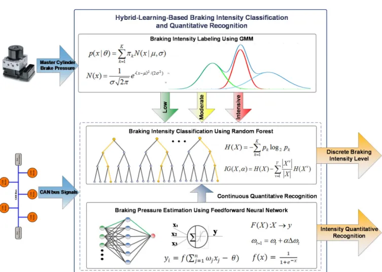
In order to realize the objectives of classification and quantitative recognition of braking intensity, the high-level methodology and related algorithms are synthesized. The algorithms are mainly comprised of three components, namely the unsupervised labelling of braking intensity level using GMM, supervised classification of braking intensity level using RF, and continuous quantitative recognition of braking intensity based on ANN. The details of the system architecture and algorithms are described as follows.
A. High-level Architecture of the Proposed Algorithms The high-level system architecture with proposed methodology are shown in Fig. 1. The GMM receives the brake pressure of master cylinder as the input, and then yields the labels of the braking intensity levels through learning. This label vector will be used as the desired output of the supervised RF learning algorithm. The RF model takes vehicle state information from CAN bus as model input, and aims to recognize the real braking intensity level without using brake pressure signals, providing a sensorless solution. Furthermore, a feedforward Neural Network (FFNN) model is used to quantitatively observe the brake intensity, which is reflected by the brake pressure exerted by driver’s operation. The FFNN takes the brake pressure as the model training label with similar input signals as used in the RF model.
This proposed methodology enables the intelligent classification and quantitative inference of driver braking intention, and it can be used to assist the advanced control and energy management for electrified vehicles, especially during regenerative braking, by augmenting the knowledge of driver’s intention and style. Detail information of CAN bus signals used for model training and testing will be described in the following sections.
B. Classification of Braking Intention Level Using GMM According to the above proposed methodology, driver’s braking intention is firstly clustered using a GMM model. GMM is a probability density function that is represented by the sum of weighted sub Gaussian components [24]. In this study, the GMM is adopted to obtain the probability distribution of the brake pressure data with an unsupervised learning approach. The brake pressure was measured in the master cylinder by a hydraulic pressure sensor. One advantage of the above proposed approach is that the GMM is an unsupervised learning method requiring no training labels and it is very flexible to select different number of clusters. In this work, there are in total three clusters generated by GMM, representing the pre-braking, moderate pre-braking, and intensive pre-braking, respectively. The series of the brake pressure data can be described as = { ⋯ }, where is the final time index. Then the GMM can be represented by the following equation:
( | ) =∑ ( | , ∑ ) (1) where is the 1-Dimensional value of brake pressure , is the parameters of GMM, is the total number of component in the model (three in this case), is the weight of each component’s Gaussian distribution function and the sum of equals to one.
3
Fig. 1. Illustration of the proposed hybrid-learning-based architecture.
( | , ∑ )is the univariate Gaussian distribution function which can be given by:
( | , ∑) = ( ) / |∑|/ exp[− ( − ) ∑ ( − )] (2)
where D is the dimension of the data vector and it is taken as 1 in this case. A complete structure of GMM, which contains three parameters, can be represented as:
= { , , ∑ } (3) Given the training data of brake pressure, the GMM can be trained with both maximum likelihood estimation (MLE) and maximum a posterior estimation (MAP). The most common method for GMM training is the Expectation-Maximization (EM) maximum likelihood estimation algorithm [25]. Suppose the training dataset of brake pressure is with the format of = {x ⋯ x }, then the overall likelihood of the GMM can be calculated by:
( | ) = ∏ ( | ) (4)
Substituting log likelihood function to Eq. (4), the above function can be transformed to a much easier one:
( ) = ∑ log ( | ) (5)
Due to the nonlinear characteristics of the log function, the utilization of the Eq. (5) makes it hardly to figure out the maximization directly. Therefore, EM is selected to compute the maximization with an iterative process, which contains two steps, i.e. the E-step and the M-step.
1) E-step: estimate the posterior probability of each component with data point .
= ∑ ( | ( ))
( | ( )) (6)
2) M-step: update the model parameters according to the estimatedposteriorprobability in E-step.
= ∑ = (7)
= ∙ = ∑∑ ∙ (8)
∑ = ( )( ) (9)
C. Braking Intention Classification Using RF
Following the above section, to learn the output label from GMM and yield accurate results correspondingly, a supervised machine learning method is then required. According to the study in [26], Random Forest algorithm achieved the best results on 121 public datasets among 179 classification
algorithms. Thus, in this study, with a great capability to accurately classify objects, the RF algorithm is used to classify and further infer the braking intention level using vehicle and powertrain signals obtained from CAN bus. And its performance of the braking intention classification will be analyzed and compared with other existing ones in the following sections.
A Random Forest is an ensemble learning method which is constructed with a combination of multiple weighted decision trees [27]. Decision tree, also known as Classification Trees and Regression Trees (CART), is a popular machine learning method that has been used in many pattern recognition and prediction tasks [28]. One decision tree is constructed with one root node, multiple middle nodes and leaf nodes. The decision results are represented by the leaf nodes in CART. Specifically, for the classification trees, the outputs are the discrete labels of the classification objects, while the outputs of regression trees are the estimated continuous values. The decision nodes and decision tree structure are determined by minimizing the information Entropy ( )and maximizing the information gain ( , ), as shown in Fig. 1. However, a single decision tree is a weak learner and has limited ability to deal with those problems with large amount of data or large dimensional feature vectors. The RF, however, parallel combines multiple trees to reduce the overfitting risk, and improves the generalization ability with the bootstrap aggregating scheme (often known as Bagging trees) [29].
RF enhances the model prediction performance by introducing the random property during model training process. Specifically, like other Bagging algorithms, RF randomly selects subset of data as training data from the original data set to train the sub decision trees. Besides, it introduce a random subset feature selection technique to avoid getting highly correlated predictors and models. Therefore, the sub decision trees will be trained with different dataset as well as different feature vectors, efficiently increasing the properties of the whole RF model. The final output of RF is the ensemble of the sub decision trees. There are mainly three ensemble methods, namely averaging, voting, and learning. A common ensemble classification algorithm is the one with weighed voting, as shown in the following.
( ) = ∑ ( ) (10)
where is the final output label, is the label set
, ⋯ ,⋯ , is learned weight of each tree output,
and ℎ( ) is the output of tree . The final output label of braking intensity will be the voting results of each sub decision trees.
D. Brake Pressure Estimation Based on ANN
According to the above analysis, discrete level estimation of the brake intensity relies on the information of brake pressure. In some modern brake systems, there are pressure sensors directly providing the measurement of brake pressure. However these sensors add considerable costs to the whole system. If the estimation technique can be achieved, realizing a sensorless braking system, then the system cost could be largely reduced. Meanwhile, the brake pressure estimation technique provides an additional redundancy for the safety-critical function of the braking system. Thus in this paper, the Artificial Neural
Networks is used to observe the continuous state of brake pressure based on vehicle and powertrain states. A multi-layer feedforward neural network (FFNN) with a hidden layer is trained to observer the brake pressure value. The architecture of the FFNN features that the information flow only has one direction and is transferred from the input layer to the output one without cycles in the model. Since the FFNN is of great ability to theoretically represent any complex polynomial function with different hidden neuron, it is selected as the model to quantitatively predict brake intention in this work.
As shown in Fig. 1, in training process, the FFNN uses both CAN bus signals and the value of brake pressure as the supervised output response. While during testing procedure, the FFNN only adopts the CAN bus signals to identify the brake pressure. The NN is construed by basic calculation units called neurons, which is inspired by human neural system. The neurons that located in different layers can be with different thresholds as well as distinguished activation functions. Neurons in each layer are interconnected with weightings. After receiving the input signals, the neurons in the hidden layer firstly sums all the weighted signals and compare it with the neuron threshold. If the summation is larger than the threshold, the neuron will be activated and outputs the processed value. The mathematical model of the neuron can be given by:
= (∑ − ) (11)
where is the output of neuron in the hidden layer, ()is the activation function, = { ⋯ }is the input from input layer, is the corresponding weight, and is the neuron threshold. A differentiable Sigmoid function is adopted as the activation function, which is with the form of:
( ) = (12)
Once the model structure is determined and parameters are initialized, the FFNN is to be trained with the method of backward propagation of error (BP). BP is an iterative NN training scheme, which consists of two basic steps including propagation and weight update. The input signals from CAN bus firstly propagate forward through the network to generate an initial estimated value, then the yield value is compared with the ground truth based on the loss function. In this study, the mean square error is utilized as the loss function.
= ∑ ( − ) (13)
where is the mean square error of the actual value and the desired one, is the total number of data samples, and are the values of ground truth and actual output, respectively.
After the propagation step, the weights of the network can be updated by calculating the gradient of the loss function. The optimal weights are expected to result in the global minimum of the loss function. Suppose that , is the weight between the input neuron and the hidden neuron , and is the output of the neuroni, then the gradient can be calculated using chain rule presented as follows:
∆
,=
,=
, (14)where∆ , is the weight gradient, and is the gradient of the sigmoid activation function shown in (13).
> REPLACE THIS LINE WITH YOUR PAPER IDENTIFICATION NUMBER (DOUBLE-CLICK HERE TO EDIT) < 5
= − ∆ (15)
where is the updated weight, is current weight, and is the learning rate of the FFNN. Eq. (15) is the simplest gradient descent updating method, more sophisticated model training algorithms for ANN can be found in [30].
III. EXPERIMENTALTESTING ANDDATAPRE-PROCESSING In order to validate the hybrid-learning-based methodology and algorithms proposed above, vehicle testing with real-world driving scenarios is required to be carried out. In this section, the experiment scenario set-up and the test vehicle will be introduced. The collected experimental data will be analyzed through signal processing methods. Besides, the selected feature vectors and model training process will be illustrated. A. Experiment Design
As Fig. 2 shows, the testing is carried out on a chassis dynamometer with an electric vehicle operating under typical driving cycles. There are a lot of standards utilized for chassis dynamometer driving cycles [31]. In this work, the New European Drive Cycle (NEDC), containing the European Union Urban Driving Cycle (ECE) and the Extra Urban Driving Cycle (EUDC), is adopted. As Fig. 3 shows, the first section of the NEDC, which is comprised of four successive ECE driving cycles, exhibits a low-speed urban operating condition. The second part, i.e. the EUDC section, represents a highway scenario with the highest speed at 120 km/h.
Fig. 2. The testing vehicle with a chassis dynamometer during experiments.
Fig. 3 Speed profile of the driving cycle with corresponding braking pressure. During testing, accessory devices such as the heater and air-conditioner need to be switched off. The battery should be fully charged with state of charge (SOC) being at 100% before the test. And the test drive requires repeated NEDC driving cycles with a maximum deviation of 2 km/h in the speed profile. Once
the vehicle is unable to follow up the target speed due to low SOC or other reasons, then the experiment will be terminated. B. Experimental Vehicle with brake blending system.
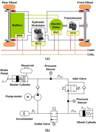
The vehicle utilized in the road tests is the electric passenger car, and the structure of the vehicle with a regenerative and hydraulic blended braking system is shown in Fig.4 (a). The front wheels of this test electric vehicle are driven by a permanent-magnet synchronous motor which can work in two states as a driving motor or a generator. The battery, which is connected to the motor through the d.c. bus, can be discharged or charged for motoring or absorbing the regenerative power during the braking process respectively. During deceleration, the blended brake torque complies to the serial regenerative strategy, i.e. the regenerative brake is applied at first, and the hydraulic brake compensates the rest part of the overall braking demand. The coordination of the blended brakes is able to guarantee the brake comfort and regeneration efficiency of the vehicle.
A schematic diagram of the hydraulic braking system is shown in Fig. 4 (b).PFW,PFWandP0denote the pressures of the master cylinder, wheel cylinder and the low-pressure accumulator, respectively. The inlet and outlet valves are respectively PWM controlled. The structure of the wheel cylinder can be simplified to a piston and spring. kFW is the equivalent stiffness of the spring and rFWis the radius of the wheel cylinder’s cross-sectional area.
Key parameters of the electrified vehicle and powertrain are listed in Table 1.
Fig. 4. Diagram of the structure of the experimental vehicle with brake system. 1000 2000 3000 4000 5000 6000 0 50 100 V eh ic le S p e e d [k m /h ] 1000 2000 3000 4000 5000 6000 0 1 2 3 4 Time [s] B ra ke P re ss u re [M P a ]
TABLE 1
KEYPARAMETERS OF THEELECTRICVEHICLEANDPOWERTRAIN.
Parameter Value Unit
Total vehicle mass 1360 kg
Wheel base 2.50 m
Frontal area 2.40 m2
Gear ratio 7.881 —
Nominal radius of tyre 0.295 m
Coefficient of air resistance 0.32 —
Motor peak power 45 kW
Motor maximum torque 144 Nm
Motor maximum speed 9000 rpm
Battery voltage 326 V
Battery capacity 66 Ah
C. Data Collection and Processing
The CAN bus data are sampled with a frequency of 100 , and 6327 seconds data are recorded in total. The raw data contains six standard NEDC driving cycles. The collected data of the vehicle speed and the brake pressure of the master cylinder are shown in Fig. 3 and further processed in Table 2.
TABLE 2
STATISTICSDATA OFVEHICLEVELOCITY ANDBRAKINGPRESSURE Variables Mean DeviationStandard Max Min
Vehicle
Velocity 35.594 km/h 30.042 km/h 118.46km/h 0 km/h Braking
Pressure 0.1857 MPa 0.4317 MPa 4.1728Mpa 0 MPa Before training and testing the models through machine learning methods, the raw data is first smoothed and filtered as follows.
= ∑ (16)
where is the value of a signal at time , is the n-th sampled value of signal at time step , and N is the total amount of samples per second.
Then, the input signals are scaled to the range from zero to one in order to eliminate the influence brought by different units.
D. Feature Selection and Model Training
In this work, the braking correlated signals and important vehicle state variables are selected for the training of the braking intensity classifier and brake pressure estimation model. The brake pressure data is only used as a response signal for FFNN training, and it is not used during the testing process. When the EV is decelerating, the electric motor works at its regenerative brake mode, recovering vehicle’s kinetic energy. During this period, the value of battery current changes from positive to negative, indicating that the battery is charged by regenerative braking energy. Thus, the signals of battery current and voltage are chosen as features. The signals that used for model training in this work are listed below in details in Table 3.
As shown in Table 3, instead of using raw data from the CAN bus only, statistical information, including the mean value, max value, and standard deviation (STD) of the original data in the past few seconds are also adopted. In this work, the values of
vehicle velocity during past five seconds are stored and used to calculate the mean and STD values. Besides, the gradient values of the battery current and voltage are also utilized.
TABLE 3
CAN BUSSIGNALSUSED FORMODELTRAINING
No. Signal No. Signal
1 Velocity ( /ℎ) 7 Acceleration ( / )
2 Accelerator Pedal Position 8 Mean Velocity ( /ℎ) 3 Battery Current ( ) 9 STD of Velocity ( /ℎ) 4 Battery Voltage ( ) 10 Max Velocity ( /ℎ) 5 Motor Speed ( / ) 11 Voltage Gradient ( / ) 6 Motor Torque ( ∙ ) 12 Current Gradient ( /)
After the feature vector being determined, the supervised classification and regression models are trained. The overall sampled data are divided into two sets, namely the training set and the testing one. The testing data set used for model training and validation contains 1400 sampled points, which is randomly chosen from the raw and training data sets. To modulate and evaluate the model performance, the K-fold cross validation approach is used. K-fold cross validation method randomly selects − 1folds from the training data to train the RF and FFNN models, and the rest fold is utilized for testing. The final assessment of the model performance is carried out according to the test results. In this work, the value of K is set as 5. Considering the data quantity and the evidence that NN with one hidden layer is able to estimate most of the complex functions, the FFNN is constructed with a hidden layer. The FFNN is then trained using a fast Levenberg-Marquardt (LM) algorithm with 5-fold cross validation.
IV. EXPERIMENTRESULTSANDANALYSIS
In this section, the experiment results of the above three machine learning tasks are described. Firstly, labeling results of braking intensity level using GMM will be illustrated. Then, classification results of the braking intensity level with the RF approach is to be presented. Finally, the results braking pressure estimation using ANN will be shown. The algorithms are implemented in Intel ® Core i7 2.5GH computer with the MATLAB 2017a platform.
A. Labeling Result of Braking Intensity Level Using GMM The Gaussian Mixture Model takes the braking pressure as an input, and it outputs the Gaussian distribution of each cluster. In order to reach good performance of the proper braking intensity identifier, a suitable GMM is achieved based on the proportion evaluation of each component. The final decision thresholds of the GMM can be given by:
= , , < 1.25, > 0.05< 0.05
ℎ, > 1.25 (17) where is the braking pressure.
Fig. 5 shows the labeling results with three different braking intensity levels. The first cluster, which is represented by the red points, is of low pressure area, representing driver’s low-intensity brake demand and the pre-braking processes. In this area, the low-level pressure is used to eliminate the mechanical gaps of brake devices. The second cluster, which is represented
> REPLACE THIS LINE WITH YOUR PAPER IDENTIFICATION NUMBER (DOUBLE-CLICK HERE TO EDIT) < 7 by yellow points with pressure range from 0.15 MPa to 1.1
MPa, indicates driver’s moderate braking intensity. And the third one indicating intensive braking is illustrated by the green points with pressure over 1.1 MPa. According to the results, the quantity of the cluster with low braking intensity is much larger than the other ones, taking up 85.3% of the overall data points. And the other two clusters share the rest of the data with similar quantities of 7.7% and 7%, respectively. The results shows a good balance maintained between the proportions and the clusters diversity.
Fig. 5 Labeling results of braking intensity levels using GMM.
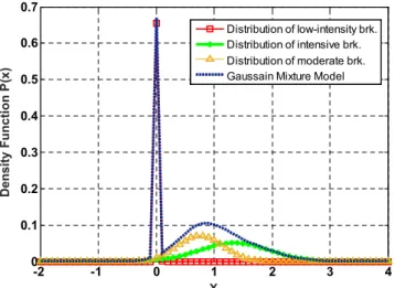
Fig. 6 illustrates the learned Gaussian distribution of the GMM with the three components. Since the low braking intensity group has much more data points and more significant characteristics, the classification confidence of this group is much higher than the other two groups. The moderate and the intensive braking levels have relatively wider Gaussian distributions and overlap with each other, showing that these two classes have similar characteristics and their data distributions can be roughly described by a single Gaussian distribution function.
Fig. 6 Gaussian distribution of GMM for braking intensity level clustering.
B. RF-Based Classification Results of Braking Intensity Level According to the above labelling, the classification results of the braking intensity level given by Random Forest is analyzed as follows. The RF classifier is constructed with 50 decision trees, and the ANN is a FFNN with 50 neurons in the hidden layer. As mentioned before, the task is to solve the three-class classification problem with the labels given by GMM. The classification performance is assessed from three different aspects, namely the classification accuracy, the execution time of model training, and the execution time of testing. The general accuracy is defined as follows.
= (18)
where is the general accuracy of the classification, is the total amount of data, , , are the number of the correct classification cases, respectively.
Moreover, the RF classifier is also compared with other existing ones, including decision trees, support vector machine, K-Nearest Neighbor and multi-layer feedforward neural networks. The detailed classification performance and comparison results are illustrated in Table 4.
TABLE4
COMPARISONRESULTS OF THEBRAKINGINTENSITYCLASSIFICATION PERFORMANCE
General
Accuracy TrainingTime (s) Testing Time(obs/sec)
Decision Tree 0.969 4.061s ~73000 Quadratic SVM 0.974 5.663s ~59000 Weighted KNN 0.967 7.818s ~12000 ANN 0.971 3.201s ~30000 Random Forest 0.977 6.086s ~27000
Fig. 7 Confusion matrix of the classification result given by RF.
The detail classification performance of the RF is illustrated using a confusion matrix, as shown in Fig. 7. The result is generated from the pre-selected 1400 data samples, containing
-2 -1 0 1 2 3 4 0 0.1 0.2 0.3 0.4 0.5 0.6 0.7 X D en si ty F u n c ti o n P (x ) Distribution of low-intensity brk. Distribution of intensive brk. Distribution of moderate brk. Gaussain Mixture Model
1 2 3 1 2 3 1227 87.6% 0 0.0% 0 0.0% 100% 0.0% 2 0.1% 91 6.5% 13 0.9% 85.8% 14.2% 0 0.0% 20 1.4% 47 3.4% 70.1% 29.9% 99.8% 0.2% 82.0% 18.0% 78.3% 21.7% 97.5% 2.5% Target Class O u tp u tC la s s Confusion Matrix
1227 low-intensity samples, 106 moderate-intensity samples, and 67 intensive ones. According to the result, cluster 1, i.e. the low-intensity braking level, achieves the result of 100% accuracy. The classification results of the second and third clusters are not as accurate as that of the first one. These fault classifications can be explained by the overlap phenomena of the Gaussian distribution of the GMM. Although there are some miss-classified occurs, their impacts on the overall system are limited, and this will be discussed in the following section.
As mentioned in Section III, the RF algorithm adopts the bootstrap method randomly selecting training data set and training predictors from raw data to construct various decision trees. In this process, about one third of the data will not being used for the model training task, and this part of the data is called the out-of-Bag (OOB) data [28]. The model testing error of the OOB data, which has a similar accuracy with real testing data, is sufficient to reflect the model generalization performance [32]. Therefore, the OOB data is used as another source to assess the model performance and estimate the importance of the predictors [32, 33].
Fig. 8 illustrates the estimation results of predictor importance with the OOB data set. It can be seen that the most important predictor in the feature vector is the battery current, following with vehicle velocity, acceleration and the standard deviation of velocity. The battery voltage, voltage variation rate, and current variation rate also exert impacts on the model classification performance.
Fig. 8 The predictor importance estimation results of Random Forest model using out-of-Bag data set.
C. Estimation Result of Braking Pressure Based on ANN The ANN-based quantitative estimation result of braking pressure is analyzed as follows. The regression result is compared with other machine learning methods, including regression decision tree, support vector machine, Gaussian process model, and regression Random Forest. The models are trained and tested with 5-fold cross validation methods. The ANN and RF have 50 neurons and trees, which are similar with the ones used in the classification task. The model performance is evaluated via four properties, namely the coefficient of determination (denote as R2), the root-mean-square-error
(RMSE), the training time, and the testing time, as shown in Table 5. R2and RMSE are common performance indexes that
has been widely accepted to evaluate the prediction accuracy.
The definitions of the R2and RMSE are presented as follows.
Suppose the ground truth data set is = { ⋯ }, and the predicted value is = { ⋯ }. The R2is calculated as:
= 1 − (19)
where is the residual sum of square, and is the total sum of square. They are defined as:
= ∑( − ) (20)
= ∑( − ) (21)
where is the mean value of the ground truth data. The RMSE can be calculated by:
= ∑ ( ) (22)
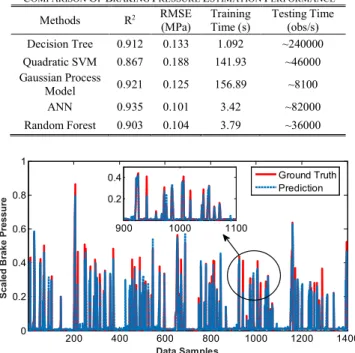
As shown in Table 5, the ANN algorithm yields the best performance of brake pressure estimation. The running time of training with ANN and RF is similar, however the testing speed of ANN is much faster than that of the RF. Another interesting phenomenon is that the single decision tree algorithm has much shorter training time and a much faster testing speed than the other algorithms. In terms of real-time application, the regression decision tree could be a better candidate because of its simplicity and high computation efficiency.
TABLE 5
COMPARISONOFBRAKINGPRESSUREESTIMATIONPERFORMANCE
Methods R2 RMSE (MPa) Training Time (s) Testing Time (obs/s) Decision Tree 0.912 0.133 1.092 ~240000 Quadratic SVM 0.867 0.188 141.93 ~46000 Gaussian Process Model 0.921 0.125 156.89 ~8100 ANN 0.935 0.101 3.42 ~82000 Random Forest 0.903 0.104 3.79 ~36000
Fig. 9 ANN-based braking pressure estimation results with 1400 testing data. The ANN model estimation result with testing data is shown in Fig. 9. The x-axis presents the 1400 data samples, and the y-axis shows the estimation results of the scaled pressure of the data samples. Since the input and output data for model training is scaled to the range of [0, 1], the model testing output is then falling within the range between 0 and 1 accordingly. Based on
Velo city Accl erat ion Peda l Curr ent Volta ge Mot orSp eed Mot orTo rque Acce lera tion Mea nVe loci ty STD Velo city Max Velo city Volta geRa te Curre ntRa te E s ti m a te s 200 400 600 800 1000 1200 1400 0 0.2 0.4 0.6 0.8 1 Data Samples S ca le d B ra ke P re ss u re 900 1000 1100 0.2 0.4 Ground Truth Prediction
> REPLACE THIS LINE WITH YOUR PAPER IDENTIFICATION NUMBER (DOUBLE-CLICK HERE TO EDIT) < 9 the results, the ANN model achieves high-precision regression
performance in most cases, and the overall root-mean-square error (RMSE) is around 0.1 MPa, demonstrating the feasibility and effectiveness of the developed algorithm.
The two most accurate models, namely the ANN and RF, are further studied in details. The impacts of different number of neurons and trees on the brake pressure prediction are analyzed. The neuron numbers of ANN and the ensemble tree numbers of RF are within the range from 10 to 100. The prediction results of the algorithms are shown in Fig. 10 and Fig. 11. According to Fig. 10, the overall performance of ANN is better than that of the RF, and the best prediction performance is yield by FFNN with number of neurons at 70. Because of using the gradient-descent-based model learning method, compared to the RF with relatively stable results, the accuracies of different FFNNs vary significantly. This shows that the prediction performance of RF changes little with different number of ensemble trees, indicating its good robustness. Fig. 11 shows the linear regression results given by the most accurate FFNN model with 70 neurons. It can be seen that the FFNN can accurately estimate the braking pressure information using vehicle states from the CAN bus.
Fig. 10 Comparison of the braking pressure estimation performance given by ANN and RF.
Fig. 11 Regression performance of FFNN with 70 neurons.
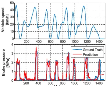
Fig. 12 Vehicle road test results of the proposed approaches.
To further validate the feasibility and effectiveness of the proposed approach, vehicle road test is carried out with the real-time implementation of the algorithms. The test track is flat and it has a dry surface with a high adhesion coefficient. As Fig. 12 shows, the road test data with a duration of 1500s contains ten individual normal deceleration processes. Among these decelerations, three typical intensities of the normal deceleration, namely the intensive, medium, and mild ones, are covered. According to the experiment results, the proposed approach is able to accurately predict the value of the brake pressure during deceleration. Comparing the prediction to the ground truth measured by onboard hydraulic pressure sensor, the values of R2 and the RMSE are over 0.85 and 0.2 MPa,
respectively, under such a naturalistic driving conditions, demonstrating the accuracy and robustness of the developed methods.
V. DISCUSSIONS
In the section, the fault classification of the intensive braking cases, which has been shown in the above section, is further analyzed based on the classification and regression results. Moreover, the methodology for improving classification and prediction performance by using a smaller feature vector, which is obtained by the predictor importance estimation result of the RF, is investigated.
A. Fault Classification of the Intensive Braking
According to the previous results in Fig. 7, the fault classifications of RF mainly occurs in the moderate and intensive braking levels. There are 13 moderate braking points that are incorrectly classified into the intensive ones, and 20 intensive cases are identified as moderate ones. From the perspective of braking safety, an intensive braking being incorrectly identified as a moderate one is much more dangerous than vice versa. Thus, the fault detection of intensive braking cases is analyzed as follows.
10 20 30 40 50 60 70 80 90 100 0.92 0.94 0.96 0.98 R S q u ar e ANN Random Forest 10 20 30 40 50 60 70 80 90 100 0.015 0.02 0.025 0.03
No. of Neurons / Trees
R M S E [M P a] ANN Random Forest 0 0.2 0.4 0.6 0.8 1 1.2 0 0.2 0.4 0.6 0.8 1 1.2 Target O u tp u t ~ = 0 .9 7 *T ar g et + 0 .0 01 1
Test Regression Result: R=0.96677
Data Fit Y = T 200 400 600 800 1000 1200 1400 0 10 20 30 40 50 V e h ic le s p e ed [k m /h ] 200 400 600 800 1000 1200 1400 0 1 2 3 4 t [s] B ra ke p re s su re [M P a ] Ground Truth Prediction
Fig. 13. The brake pressure estimation result of the intensive braking cases. There are 67 intensive braking samples within the testing dataset, among which 20 cases is of fault classification and 47 are correct ones. Fig. 13 shows the braking pressure prediction results of the total 67 samples using ANN algorithm. The upper and lower subplots present the fault and correct classification cases, respectively. As the upper subplot shows, the braking pressure of the fault classifications is mainly located within the range from 0.3 to 0.4, corresponding to 1.2 MPa-1.6MPa in real measurement. However, this above pressure range is around the lower bound of the overall intensive braking samples, so it can be accepted to be classified into the moderate level group. Besides, most of the estimated pressure point generated by the trained FFNN model can accurately follow the real value. Therefore, we believe that the 20 fault classification samples have small effects on the whole intensive braking process. B. Performance with a Reduced Order Feature Vector
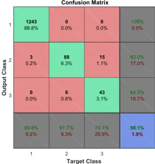
According to the analysis results illustrated in Fig. 8, the four most important predictors of the raw data for classification are: the battery current, the vehicle speed, the acceleration, and the standard deviation of the speed. In order to extend the proposed approach to conventional internal combustion engine (ICE) vehicles by removing signals related to electric powertrains, in this section, a new feature vector and dataset containing only the above four signals are constructed and adopted to assess the classification and prediction performance. The confusion matrix of the classification and the predicted braking pressures with the new feature vector and dataset are illustrated in Fig. 14 and Fig. 15, respectively.
As shown in Fig. 14, the new RF model, which is trained with a low dimensional dataset, generates more accurate classification results. The classifier is tested with 1400 randomly selected testing data points. The accuracies of the moderate and intensive braking classification results are improved from 85.8% to 91.7% and from 70.1% to 74.1%, respectively.
Fig. 14. Braking intensity classification results given by RF using a lower dimensional feature vector with 50 ensemble trees.
The estimation results of the braking pressure with the FFNN model is shown in Fig. 15. Due to the dimension reduction, the prediction accuracy of the FFNN slightly decreases. The values of R2and RMSE of the testing dataset become 0.905 and
0.123MPa. Although the braking pressure prediction performance reduces, the FFNN model is still able to estimate braking pressure with small errors in most of the situations, indicating that that the proposed approach can be applied in conventional ICE vehicles.
Fig. 15. Braking pressure prediction result given by FFNN using a reduced dimensional feature vector with 50 neurons.
VI. CONCLUSIONS
In this paper, a hybrid-learning-based classification and quantitative recognition methodology of driver braking intensity is investigated. Three different braking intensity levels, namely the low-intensity, the moderate and intensive braking, are firstly identified using GMM algorithm. Then, a Random Forest algorithm is proposed to classify the braking intensity level based on the output label of GMM and vehicle state variables from CAN bus. Finally, a continuous estimation algorithm for braking pressure observation using Feedforward
2 4 6 8 10 12 14 16 18 20 0.2 0.3 0.4 S ca le d P re s su re
Fault Classification of Intensive Braking Data
Data Sample Ground Truth Prediction 5 10 15 20 25 30 35 40 45 50 0.2 0.4 0.6 0.8 Data Sample S ca le d P re s su re
Correct Classification of Intensive Braking Data
Ground Truth Prediction 1 2 3 Target Class 1 2 3 O u tp u t C la ss Confusion Matrix 1243 88.8% 3 0.2% 0 0.0% 99.8% 0.2% 0 0.0% 88 6.3% 8 0.6% 91.7% 8.3% 0 0.0% 15 1.1% 43 3.1% 74.1% 25.9% 100% 0.0% 83.0% 17.0% 84.3% 15.7% 98.1% 1.9% 0 200 400 600 800 1000 1200 1400 0 0.1 0.2 0.3 0.4 0.5 0.6 0.7 0.8 Data Samples S c a le d B ra k in g P re s s u re Ground Truth Prediction
> REPLACE THIS LINE WITH YOUR PAPER IDENTIFICATION NUMBER (DOUBLE-CLICK HERE TO EDIT) < 11 Neural Network is proposed. High-accuracy results of the
braking intensity classification and brake pressure prediction are achieved with the developed hybrid machine learning methods. In order to validate the algorithms, experimental data are firstly collected from an electric vehicle under standard NEDC driving cycles. Then, the hybrid learning methods are tested and improved with the collected dataset. The testing results show that the proposed methods, which require simple modelling and parameter identification procedures, are able to accurately classify the braking intensity levels and predict the braking pressure correspondingly. It enables the sensorless technology and provides an additional redundancy for the safety-critical braking system, and it can be widely utilized in energy management and active chassis control for various types of ground vehicles.
REFERENCES
[1] C. Lv, D. Cao, Y. Zhao, D. J. Auger, et al., "Analysis of autopilot disengagements occurring during autonomous vehicle testing," IEEE/CAA Journal of Automatica Sinica, vol. 5, pp. 58-68, 2018. [2] Mallik, Ayan, Weisheng Ding, and Alireza Khaligh. "A Comprehensive
Design Approach to an EMI Filter for a 6-kW Three-Phase Boost Power Factor Correction Rectifier in Avionics Vehicular Systems." IEEE Transactions on Vehicular Technology 66, no. 4 (2017): 2942-2951. [3] Zhang, Hui, and Junmin Wang. "Active steering actuator fault detection
for an automatically-steered electric ground vehicle." IEEE Transactions on Vehicular Technology 66, no. 5 (2017): 3685-3702.
[4] Yu, Liang, Haoyu Wang, and Alireza Khaligh. "A Discontinuous Conduction Mode Single-Stage Step-Up Rectifier for Low-Voltage Energy Harvesting Applications." IEEE Transactions on Power Electronics 32, no. 8 (2017): 6161-6169.
[5] Li, Nanxiang, Teruhisa Misu, and Fei Tao. "Understand driver awareness through brake behavior analysis: Reactive versus intended hard brake." In Intelligent Vehicles Symposium (IV), 2017 IEEE, pp. 1523-1528. IEEE, 2017.
[6] Zeng, Xiangrui, and Junmin Wang. "A Stochastic Driver Pedal Behavior Model Incorporating Road Information." IEEE Transactions on Human-Machine Systems (2017).
[7] Lorenzo, Beatriz, Francisco Javier Gonzalez-Castano, and Yuguang Fang. "A Novel Collaborative Cognitive Dynamic Network Architecture." IEEE Wireless Communications 24, no. 1 (2017): 74-81.
[8] Martinez, C. M., Hu, X., Cao, D., et al. "Energy Management in Plug-in Hybrid Electric Vehicles: Recent Progress and a Connected Vehicles Perspective." IEEE Transactions on Vehicular Technology, vol. 66, pp. 4534-4549, 2017.
[9] Schnelle, Scott, Junmin Wang, Haijun Su, and Richard Jagacinski. "A driver steering model with personalized desired path generation." IEEE Transactions on Systems, Man, and Cybernetics: Systems 47, no. 1 (2017): 111-120.
[10] Lv, C., Zhang, J. and Li, Y. "Extended-Kalman-filter-based regenerative and friction blended braking control for electric vehicle equipped with axle motor considering damping and elastic properties of electric powertrain." Vehicle System Dynamics 52, no. 11 (2014): 1372-1388. [11] Ivanov, Valentin, Dzmitry Savitski, and Barys Shyrokau. "A survey of
traction control and antilock braking systems of full electric vehicles with individually controlled electric motors." IEEE Transactions on Vehicular Technology 64, no. 9 (2015): 3878-3896.
[12] Lv, C., Zhang, J., Li, Y. and Yuan, Y. "Directional-stability-aware brake blending control synthesis for over-actuated electric vehicles during straight-line deceleration." Mechatronics 38 (2016): 121-131.
[13] Zhang, J., Lv, C., Gou, J. and Kong, D. "Cooperative control of regenerative braking and hydraulic braking of an electrified passenger car." Proceedings of the Institution of Mechanical Engineers, Part D: Journal of Automobile Engineering 226, no. 10 (2012): 1289-1302. [14] Lv, Chen, Junzhi Zhang, Yutong Li, and Ye Yuan. "Novel control
algorithm of braking energy regeneration system for an electric vehicle during safety–critical driving maneuvers." Energy conversion and management 106 (2015): 520-529.
[15] C. Lv, Y. Xing, J. Zhang, X. Na, Y. Li, T. Liu, et al., "Levenberg-Marquardt Backpropagation Training of Multilayer Neural Networks for State Estimation of A Safety Critical Cyber-Physical System," IEEE Transactions on Industrial Informatics, 2017.
[16] C. Lv, Y. Liu, X. Hu, et al, "Simultaneous Observation of Hybrid States for Cyber-Physical Systems: A Case Study of Electric Vehicle Powertrain," IEEE Transactions on Cybernetics, 2017.
[17] Lv, C., Wang, H., and Cao, D. "High-Precision Hydraulic Pressure Control Based on Linear Pressure-Drop Modulation in Valve Critical Equilibrium State." IEEE Transactions on Industrial Electronics, 2017. [18] Haufe, S. Kim, J.-W. Kim, I.-H. Sonnleitner, A. Schrauf, M. Curio, and
G. Blankertz, B. “Electrophysiology-based detection of emergency braking intention in real-world driving.,” J. Neural Eng., vol. 11, no. 5, p. 056011, 2014.
[19] Suzuki, Hironori. "Prediction of Driver's Brake Pedal Operation in Vehicle Platoon System: Model Development and Proposal." Intelligent Systems, Modelling and Simulation (ISMS), 2016 7th International Conference on. IEEE, 2016.
[20] Wang, Jianqiang, et al. "An adaptive longitudinal driving assistance system based on driver characteristics." IEEE Transactions on Intelligent Transportation Systems 14.1 (2013): 1-12.
[21] Jiang, Guirong, et al. "Real-time estimation of the pressure in the wheel cylinder with a hydraulic control unit in the vehicle braking control system based on the extended Kalman filter." Proceedings of the Institution of Mechanical Engineers, Part D: Journal of Automobile Engineering (2016): 0954407016671685.
[22] Sankavaram, Chaitanya, et al. "Fault diagnosis in hybrid electric vehicle regenerative braking system." IEEE Access 2 (2014): 1225-1239. [23] Song, Yantao, and Bingsen Wang. "Analysis and experimental
verification of a fault-tolerant HEV powertrain." IEEE Transactions on Power Electronics 28.12 (2013): 5854-5864.
[24] Rasmussen, Carl Edward. "The infinite Gaussian mixture model." NIPS. Vol. 12. 1999.
[25] Xuan, Guorong, Wei Zhang, and Peiqi Chai. "EM algorithms of Gaussian mixture model and hidden Markov model." Image Processing, 2001. Proceedings. 2001 International Conference on. Vol. 1. IEEE, 2001. [26] Fernández-Delgado, Manuel, et al. "Do we need hundreds of classifiers to
solve real world classification problems." J. Mach. Learn. Res 15.1 (2014): 3133-3181.
[27] Breiman, Leo. "Random forests." Machine learning 45.1 (2001): 5-32. [28] Safavian, S. Rasoul, and David Landgrebe. "A survey of decision tree
classifier methodology." IEEE transactions on systems, man, and cybernetics 21.3 (1991): 660-674.
[29] Breiman, Leo. "Bagging predictors." Machine learning 24.2 (1996): 123-140.
[30] Demuth, Howard B., et al. Perception Learning Rule, in Neural network design. Martin Hagan, 2014.
[31] Lv, Chen, Junzhi Zhang, Yutong Li, and Ye Yuan. "Mechanism analysis and evaluation methodology of regenerative braking contribution to energy efficiency improvement of electrified vehicles." Energy Conversion and Management 92 (2015): 469-482.
[32] Wolpert, David H., and William G. Macready. "An efficient method to estimate bagging's generalization error." Machine Learning 35.1 (1999): 41-55.
[33] Loh, Wei-Yin, and Yu-Shan Shih. "Split selection methods for classification trees." Statistica sinica (1997): 815-840.
Chen Lvis currently a Research Fellow at Advanced Vehicle Engineering Center, Cranfield University, UK. He received the Ph.D. degree at Department of Automotive Engineering, Tsinghua University, China in 2016. From 2014 to 2015, he was a joint PhD researcher at EECS Dept., University of California, Berkeley. His research focuses on cyber-physical system, hybrid system, advanced vehicle control and intelligence, where he has contributed over 40 papers and obtained 11 granted China patents. Dr. Lv serves as a Guest Editor for IEEE/ASME Transactions on Mechatronics, IEEE Transactions on Industrial Informatics and International Journal of Powertrains, and an Associate Editor for International Journal of Electric and Hybrid Vehicles, International Journal of Vehicle Systems Modelling and Testing, International Journal of Science and Engineering for Smart Vehicles, and Journal of Advances in Vehicle Engineering. He received the Highly Commended Paper Award of IMechE UK
in 2012, the National Fellowship for Doctoral Student in 2013, the NSK Outstanding Mechanical Engineering Paper Award in 2014, the Tsinghua University Graduate Student Academic Rising Star Nomination Award in 2015, the China SAE Outstanding Paper Award in 2015, the 1stClass Award of China Automotive Industry Scientific and Technological Invention in 2015, and the Tsinghua University Outstanding Doctoral Thesis Award in 2016.
Yang Xingreceived his B.S. in Automatic Control from Qingdao University of Science and Technology, Shandong, China, in 2012. He then received his Msc. with distinction in Control Systems from the department of Automatic Control and System Engineering, The University of Sheffield, UK, in 2014. Now he is a Ph. D. candidate for Transport Systems, Cranfield University, UK. His research interests include driver behaviour modelling, driver-vehicle interaction, and advance driver assistance systems. His work focuses on the understanding of driver behaviours and identification of driver intentions using machine-learning methods for intelligent and automated vehicles.
Chao Lureceived his Ph.D. degree from University of Leeds, UK in 2015. He is currently a visiting researcher at the Advanced Vehicle Engineering Centre, Cranfield University, UK, and a Lecturer at the School of Mechanical Engineering, Beijing Institute of Technology, China. His research interests include Intelligent Transportation Systems, automated driving, and reinforcement learning. Yahui Liureceived his B.S. degree from Jilin University, China, in 2003 and Ph.D. degree from Beihang University, China, in 2009 respectively. He is currently an Associate Professor at State Key Laboratory of Automotive Safety and Energy, Tsinghua University, China. His research interests include driver-vehicle system dynamics, steering system, and actuator design of ADAS.
Hongyan Guoreceived the B.S. and M.S. degrees from the University of Science and Technology Liaoning, Anshan, China, in 2004 and 2007, respectively, and the Ph.D. degree from Jilin University, Changchun, China, in 2010. Currently, she is an Associate Professor with the Department of Control Science and Engineering, Jilin University. Her current research interests include vehicle states estimation and stability controls.
Hongbo Gaois currently a postdoctoral student at Dept. of Automotive Engineering, Tsinghua University, China. His research interests include intelligent vehicles, intelligent transportation systems, and automated driving.
Dongpu Caoreceived the Ph.D. degree from Concordia University, Canada, in 2008. He is currently an Associate Professor at Mechanical and Mechatronics Engineering, University of Waterloo, Canada. His research focuses on vehicle dynamics and control, automated driving and parallel driving, where he has contributed more than 100 publications and 1 US patent. He received the ASME AVTT’2010 Best Paper Award and 2012 SAE Arch T. Colwell Merit Award. Dr. Cao serves as an Associate Editor for IEEE TRANSACTIONS ON INTELLIGENT TRANSPORTATION SYSTEMS, IEEE TRANSACTIONS ON VEHICULAR TECHNOLOGY, IEEE TRANSACTIONS ON INDUSTRIAL ELECTRONICS, IEEE/ASME TRANSACTIONS ON MECHATRONICS and ASME JOURNAL OF DYNAMIC SYSTEMS, MEASUREMENT, AND CONTROL. He has been a Guest Editor for VEHICLE SYSTEM DYNAMICS, and IEEE
TRANSACTIONS ON HUMAN-MACHINE SYSTEMS. He serves on the SAE International Vehicle Dynamics Standards Committee and a few ASME, SAE, IEEE technical committees.