Learning Label Structures
with Neural Networks for
Multi-label Classification
Vom Fachbereich Informatik der Technischen Universität Darmstadtzur Erlangung des Grades eines Doktors der Naturwissenschaften (Dr. rer. nat.) genehmigteDissertationvonJinseok Nam, M.Sc. aus Tae-baek
Tag der Einreichung: 02. Mai 2018 Tag der Verteidigung: 11. Juni 2018 Darmstadt 2019 – D 17
1. Referent: Prof. Dr. Johannes Fürnkranz 2. Referent: Prof. Dr. Krzysztof Dembczy´nski
Learning Label Structures with Neural Networks for Multi-label Classification
GenehmigteDissertationvonJinseok Nam, M.Sc. aus Tae-baek 1. Referent: Prof. Dr. Johannes Fürnkranz
2. Referent: Prof. Dr. Krzysztof Dembczy´nski Tag der Einreichung: 02. Mai 2018
Tag der Verteidigung: 11. Juni 2018 Darmstadt 2019 – D17
Please cite this document as
URN: urn:nbn:de:tuda-tuprints-87385
URL: http://tuprints.ulb.tu-darmstadt.de/8738 This document is provided by tuprints, E-Publishing-Service of the TU Darmstadt http://tuprints.ulb.tu-darmstadt.de
This work is published under the following Creative Commons license: Attribution – Non Commercial – No Derivative Works 4.0 International http://creativecommons.org/licenses/by-nc-nd/4.0/
Zusammenfassung
Multi-Label-Klassifizierung (MLC) bezeichnet die Aufgabe, eine Menge von Labels für eine gegebene Instanz vorherzusagen. Eine zentrale Herausforderung bei MLC ist die Erfassung der zugrundeliegenden Strukturen im Labelraum. Aufgrund der Komplexität des Lernens aus allen möglichen Labelkombinationen ist es bei großen MLC Datensätzen von entschei-dender Bedeutung, sowohl Skalierbarkeit als auch Vorhersagequalität zu berücksichtigen. Ein weiteres Problem, das bei der Erstellung von MLC-Systemen auftritt, ist die Frage nach dem Evaluationsmaß, welches für den Vergleich der Vorhersagequalität herangezogen werden soll. Im Gegensatz zur traditionellen Multi-Klassen-Klassifizierung werden in MLC häufig mehre-re Evaluationsmaße gemeinsam eingesetzt, da jedes Maß ein andemehre-res MLC-System präferiert. Mit anderen Worten, es ist entscheidend, die Eigenschaften der verschiedenen MLC Evalua-tionsmaße zu verstehen, um ein System zu erstellen, das gut in Bezug auf die Maße ist, an denen wir besonders interessiert sind.
In dieser Arbeit entwickeln wir Architekturen von Neuronalen Netzwerken (NN), die La-belstrukturen in großen MLC-Problemen effizient und effektiv bezüglich eines bestimmten Evaluationsmaßes ausnutzen. Obwohl NNs, die aus paarweisen Labelbeziehungen lernen, bereits länger in der Literatur verwendet werden, schlagen wir eine vergleichsweise simple Architektur vor, die eine Verlustfunktion verwendet, die Label-Abhängigkeiten ignoriert. Wir zeigen, dass unser Ansatz besser funktioniert als komplexere neuronale Netze bezüglich des Rank-Loss-Maßes, welches explizit die Anzahl der durch das Verfahren falsch sortierten Labelpaare berücksichtigt.
Ein weiteres Evaluationsmaß, das üblicherweise beachtet wird, ist Subset 0/1-Loss. Der Classifier-Chain-Ansatz (CC) ist ein erfolgreiches, aktuelles Verfahren um dieses Maß zu optimieren. Dies geschieht dadurch, dass das ursprüngliche Problem in ein sequentielles Vorhersageproblem umgewandelt wird, sodass die Aufgabe daraufhin darin besteht, eine Sequenz von Binärwerten für die Labels vorherzusagen. Im Gegensatz zur eben genannten NN-Architektur, die Labelstrukturen ignoriert, setzen wir rekurrente neuronale Netze (RNN) ein, um Sequenzstrukturen in den Labelketten auszunutzen. Die vorgeschlagenen RNNs er-weisen sich gegenüber CCs als vorteilhaft bei Problemen mit einer großen Anzahl an Labels wegen Parameter-Sharing-Effekten bei RNNs und bei Problemen mit langen Labelsequenzen. Zusätzlich zu den NNs, die auf Labelsequenzen gelernt werden, stellen wir zwei weite-re neuartige NN-basierte Methoden vor. Diese Methoden projizieweite-ren sowohl Instanzen als auch Labels auf eine Art und Weise in einen gemeinsamen niedrig-dimensionalen Raum, welche die Distanz zwischen einer Instanz und ihren relevanten Labels in diesem Raum reduziert. Während das Ziel beider Lernmethoden gleich ist, nämlich das Projizieren von Instanzen und Labels in einen gemeinsamen Raum, verwenden sie unterschiedliche Zusatz-informationen über die Labelräume: Das erste vorgeschlagene Verfahren nutzt hierarchische Strukturen aus und kann insbesondere nützlich sein, wenn solche Stukturen von Experten zur Verfügung gestellt werden. Die zweite Methode nutzt latente Labelräume aus, die von den textuellen Beschreibungen der Labels gelernt werden, sodass wir das Verfahren auf allgemei-nere MLC-Probleme anwenden können, für die keine expliziten Labelstrukturen vorhanden
sind. Ungeachtet der Unterschiede ermöglichen uns beide Verfahren, Vorhersagen über La-bels zu treffen, die während des Trainings nicht gesehen wurden. Außerdem zeigen wir, dass beide Verfahren in der Lage sind, durch Ausnutzung der Zusatzinformationen insgesamt eine bessere Vorhersagequalität zu erreichen.
Abstract
Multi-label classification (MLC) is the task of predicting a set of labels for a given input instance. A key challenge in MLC is how to capture underlying structures in label spaces. Due to the computational cost of learning from all possible label combinations, it is crucial to take into account scalability as well as predictive performance when we deal with large-scale MLC problems. Another problem that arises when building MLC systems is which evaluation measures need to be used for performance comparison. Unlike traditional multi-class multi-classification, several evaluation measures are often used together in MLC because each measure prefers a different MLC system. In other words, we need to understand the properties of MLC evaluation measures and build a system which performs well in terms of those evaluation measures in which we are particularly interested.
In this thesis, we develop neural network architectures that efficiently and effectively utilize underlying label structures in large-scale MLC problems. In the literature, neural networks (NNs) that learn from pairwise relationships between labels have been used, but they do not scale well on large-scale label spaces. Thus, we propose a comparably simple NN architecture that uses a loss function which ignores label dependencies. We demonstrate that simpler NNs using cross-entropy per label works better than more complex NNs, particularly in terms of rank loss, an evaluation measure that takes into account the number of incorrectly ranked label pairs.
Another commonly considered evaluation measure is subset 0/1 loss. Classifier chains (CCs) have shown state-of-the-art performance in terms of that measure because the joint probability of labels is optimized explicitly. CCs essentially convert the problem of learning the joint probability into a sequential prediction problem. Then, the task is to predict a sequence of binary values for labels. Contrary to the aforementioned NN architecture which ignores label structures, we study recurrent neural networks (RNNs) so as to make use of sequential structures on label chains. The proposed RNNs are advantageous over CC approaches when dealing with a large number of labels due to parameter sharing effects in RNNs and their abilities to learn from long sequences. Our experimental results also confirm that their superior performance on very large label spaces.
In addition to NNs that learn from label sequences, we present two novel NN-based meth-ods that learn a joint space of instances and labels efficiently while exploiting label structures. The proposed joint space learning methods project both instances and labels into a lower dimensional space in a way that minimizes the distance between an instance and its relevant labels in that space. While the goal of both joint space learning methods is same, they use different additional information on label spaces during training: One approach makes use of hierarchical structures of labels and can be useful when such label structures are given by human experts. The other uses latent label spaces learned from textual label descriptions so that we can apply it to more general MLC problems where no explicit label structures are available. Notwithstanding the difference between the two approaches, both approaches allow us to make predictions with respect to labels that have not been seen during training.
Acknowledgements
I would like to express my sincere appreciation to my advisor Professor Dr. Johannes Fürnkranz. He has taught me how to develop solid research questions and encouraged me to pursue interesting research directions that has helped me grow as a researcher. He gave me thought provoking advice when I needed his help and his guidance has been invalu-able. I am also grateful for his time, endless support and patience to keep me motivated and make my Ph.D. study more productive.
I would also like to thank Dr. Eneldo Loza Mencïa. As an expert in the field of multi-label learning and also my lab mate, he has spent his time for discussion with me from which I was able to develop a better insight into multi-label problems and solutions. All the discussions I had with him were fruitful and motivational for me.
I would also like to thank my committee members, Professor Dr. Krzysztof Dembczyński, Professor Dr. Iryna Gurevych, Professor Dr. Kristian Kersting and Professor Dr. Ar-jan Kuijper for serving as my committee members and giving me insightful comments and suggestions.
The members of Knowledge Engineering group have also contributed to my personal and professional time at TU Darmstadt. The events organized by the members for fun were enjoyable and made me feel at home even when I was stuck during my journey toward scientific goals.
I gratefully acknowledge the funding sources. I was funded by the German Institute for International Educational Research under the Knowledge Discovery and Scientific Liter-ature program and the German Research Foundation under the Adaptive Preparation of Information from Heterogeneous Sources program (AIPHES, GRK 1994/1). My scientific contributions would not be made possible without their generous financial support.
Last but not least, I would like to express my deepest gratitude to my wife YoonAh for her faithful support during my Ph.D. study since its beginning.
Contents
1 Introduction 1
1.1 Summary of Contributions . . . 4
1.2 Thesis Outline . . . 4
2 Background 7 2.1 Binary Classification and Risk Minimization . . . 7
2.2 Multi-label Classification . . . 9
2.2.1 Evaluation Measures for Multi-label Classification . . . 12
2.2.2 Risk Minimization for Multi-label Classification . . . 14
2.2.3 Multi-label Learning Algorithms . . . 17
2.3 Fundamentals of Neural Networks . . . 22
2.3.1 Feed-forward Neural Networks . . . 22
2.3.2 Neural Language Modeling . . . 27
2.3.3 Recurrent Neural Networks . . . 30
2.3.4 Neural Machine Translation . . . 36
3 Efficient Neural Networks for Large-scale Multi-label Classification 41 3.1 Introduction . . . 41
3.2 Neural Networks for Multi-label Classification . . . 42
3.2.1 Rank Loss . . . 42
3.2.2 Pairwise Ranking Loss Minimization in Neural Networks . . . 42
3.2.3 Thresholding . . . 44
3.2.4 Ranking Loss vs. Cross Entropy . . . 44
3.2.5 Recent Advances in Deep Learning . . . 46
3.3 Experimental Setup . . . 48
3.4 Results . . . 49
3.5 Conclusion . . . 52
4 Estimating Joint Probabilities of Label Subsets using Label Sequences 55 4.1 Introduction . . . 55
4.2 Learning to Predict Subsets as Sequence Prediction . . . 56
4.2.1 Determining Label Permutations . . . 57
4.2.2 Label Sequence Prediction from Given Label Permutations . . . 57
4.3 Experimental Setup . . . 60
4.3.1 Baselines and Training Details . . . 60
4.3.2 Datasets and Preprocessing . . . 61
4.4 Experimental Results . . . 61
4.4.1 Experiments on Reuters-21578 . . . 62
4.4.3 Experiments on BioASQ . . . 65
4.5 Conclusion . . . 68
5 Learning from Label Hierarchies 69 5.1 Introduction . . . 69
5.2 Model Description . . . 70
5.2.1 Joint space embeddings . . . 70
5.2.2 Learning with hierarchical structures over labels . . . 71
5.2.3 Label ranking to binary predictions . . . 73
5.3 Experimental Setup . . . 73
5.4 Experimental Results . . . 76
5.4.1 Learning All Labels Together . . . 76
5.4.2 Learning to Predict Unseen Labels . . . 77
5.5 Pretrained Label Embeddings as Good Initial Guess . . . 77
5.5.1 Encoding Hierarchical Structures . . . 78
5.5.2 Understanding Label Embeddings . . . 80
5.5.3 Different Hierarchies, Different Representations . . . 83
5.5.4 Results . . . 84
5.6 Conclusions . . . 84
6 Discovering Latent Structures from Label Descriptions 87 6.1 Introduction . . . 87
6.2 Problem Statement . . . 88
6.3 Method . . . 89
6.3.1 Documents and Labels as Word Sequences . . . 89
6.3.2 Joint Embeddings . . . 90
6.3.3 Putting It All Together . . . 91
6.3.4 Inference on Unseen Documents and Labels . . . 92
6.4 Experimental Setup . . . 93
6.4.1 Dataset . . . 94
6.4.2 Baseline . . . 94
6.5 Experiments . . . 94
6.5.1 Effect of Label Descriptions . . . 95
6.5.2 Unseen Label Representations . . . 96
6.5.3 Zero-Shot Prediction . . . 97
6.6 Discussion . . . 99
7 Conclusions and Future Work 101
List of Abbreviations
1-err one error 13ACC subset accuracy12,13, 15, 62, 63,65, 67
ANN artificial neural networkxi, 22
AvgP average precision 13
BP-MLL backpropagation for multi-label learning3, 18, 41, 43–46
BR binary relevance17, 18, 41, 60,63, 65
C2AE canonical-correlated autoencoder21
CBM conditional Bernoulli mixture19
CC classifier chainiii, 55, 56, 60, 101
CCA canonical correlation analysis21
CE cross entropy 45, 46
CML collective multi-label classifier 19
CMLF collective multi-label with feature classifier 19
Cov coverage13
CPLST conditional principal label space transformation20, 21
CRF conditional random field 19
CS compressed sensing20
DAG directed acyclic graph 57, 61
DFS depth-first search 57, 61
DNN deep neural network2,3, 21
ebF1 example-basedF1-measure 13,62, 63, 65, 67 EncDec encoder-decoder37, 38, 58–63,65–68
FaIE feature-aware implicit label space encoding 21
FNN feed-forward neural network2,5, 22–24, 27, 30, 31,55
GPU graphics processing unit 3
GRU gated recurrent unit36–38, 58, 60
HA Hamming accuracy 12, 15,62, 63, 65, 67
HMLC hierarchical multi-label classification20
KN Kneser-Ney29
LEML low-rank risk minimization for multi-label learning 21
LM language model 27, 29
LP label powerset 18, 55,56, 60, 63, 65,101
LR logistic regression2, 18
LSDR label space dimensionality reduction21
LSTM long short-term memory32–38
maF1 macro-averaged F1 14, 62, 63, 65,67 miF1 micro-averagedF1 14, 62, 63,65, 67
MLC multi-label classification iii, xiii, 1–7, 9–14, 17–21, 29, 41, 42, 55–61, 65,
MLP multi-layer perceptron 22, 30
MLTC multi-label text classification 5, 102
NLL negative log-likelihood62
NLM neural language model 27, 29
NMT neural machine translation 36,39
NN neural network iii, 2–6, 18, 28–30, 41, 42, 44, 45, 47, 48, 57, 58, 60, 63,
65, 101
OOV out-of-vocabulary 36, 37,61
PCC probabilistic classifier chain 5, 19, 55–60,63, 65, 68
PLST principal label space transformation 20, 21
PLT probabilistic label tree 22
PWE pairwise error function 43–46
ReLU rectified linear unit 41, 47
REML robust extreme multi-label learning21
RL rank loss 13
RNN recurrent neural network iii, xiii, 5,30–34, 36–38, 56–62, 68,101,102
Seq2Seq sequence-to-sequence 58
SGD stochastic gradient descent 47
SLEEC sparse local embeddings for extreme multi-label classification 21
SVD singular value decomposition20
SVM support vector machine18,41, 42
tf-idf term frequency-inverse document frequency 41, 48
tSNE t-distributed stochastic neighbor embedding78, 79, 97
WARP weighted approximate-rank pairwise90,92, 94
XMLC extreme multi-label classification 21, 102
List of Figures
1.1 A real-world example of multi-label data . . . 2
1.2 Illustration of zero-shot learning. . . 4
2.1 Illustration of the regret decomposition. . . 9
2.2 Estimation and approximation errors . . . 10
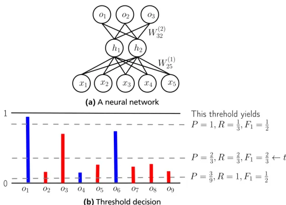
2.3 Directed graph representing a simpleartificial neural network . . . 22
2.4 Feed-forward neural network . . . 23
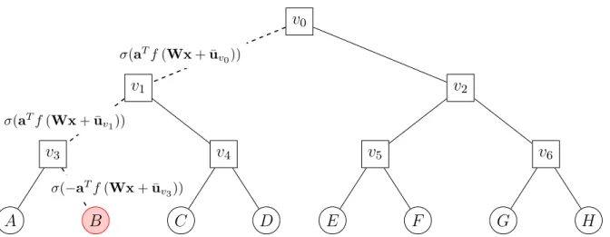
2.5 How hierarchical softmax works . . . 28
2.6 Recurrent neural network . . . 30
2.7 Gradient computation in recurrent neural networks . . . 31
3.1 Threshold adjustment for F1 score maximization . . . 43
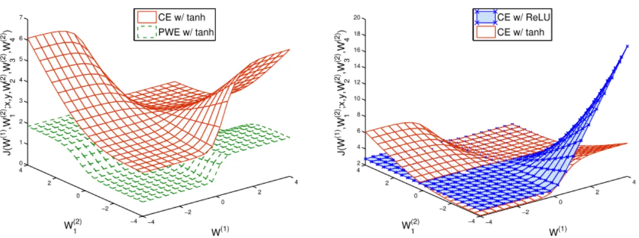
3.2 Comparison of landscape of the cost functions and a type of hidden unit . . . 46
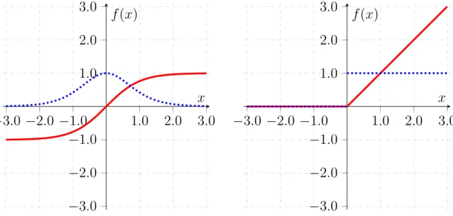
3.3 Activation functions and their derivative . . . 47
3.4 Effect of gradient descent algorithms and dropout . . . 50
3.5 Comparison of two cost functions . . . 51
4.1 Illustration of PCC and RNN architectures for MLC . . . 59
4.2 Negative log-likelihood on Reuters-21578 . . . 62
4.3 Performance of RNNs in terms of various evaluation measures . . . 64
4.4 Comparison of two RNN architectures in terms of the number of positive labels 66 5.1 Illustration of joint space learning with label structures . . . 72
5.2 Learned representations of 16 major categories in MeSH vocabulary . . . 79
5.3 Label embedding spaces learned with and without label structures . . . 80
5.4 Learned label embeddings in 2D space . . . 81
5.5 Effect of label hierarchy in learned label embeddings . . . 83
6.1 Illustration of AiTextML. . . 92
6.2 AiTextML at inference time . . . 93
6.3 Effect of learning from label descriptions . . . 95
6.4 Relative improvement of AiTextML in terms of label frequencies . . . 96
List of Tables
2.1 An example of multi-label instances . . . 10
2.2 An example of the joint probability of two labels . . . 11
2.3 Example-based evaluation . . . 12
2.4 Label-based evaluation . . . 14
2.5 Examples of theBayes classifiers . . . 17
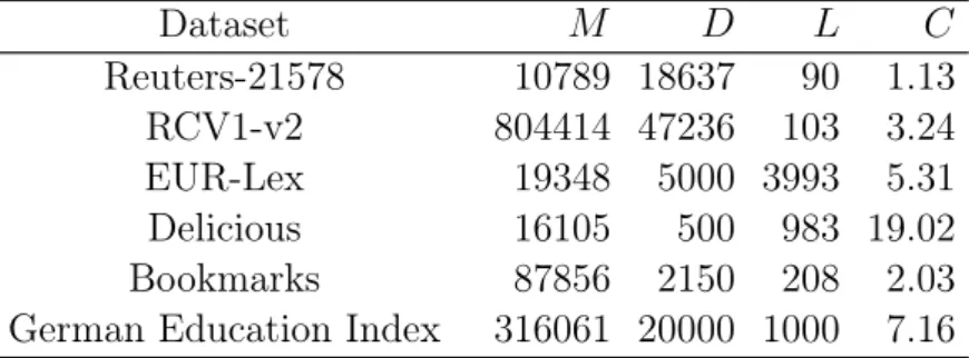
3.1 Statistics of the datasets used in the experiments . . . 49
3.2 Average ranks of the algorithms on ranking and bipartition measures. . . 52
3.3 Results on ranking and bipartition measures . . . 53
4.1 Comparison of the three RNN architectures for MLC. . . 60
4.2 Statistics of the datasets used in the epxeriments . . . 61
4.3 Performance comparison on Reuters-21578. . . 63
4.4 Performance comparison on RCV1-v2. . . 65
4.5 Performance comparison on BioASQ. . . 67
5.1 Statistics of the datasets used in the experiments . . . 74
5.2 Comparison of WsabieH to its baselines . . . 76
5.3 Comparison of WsabieH compared to its baseline . . . 77
5.4 Analogical reasoning on learned vector representations of MeSH vocabulary . 82 5.5 Initialization of label embeddings on OHSUMED underzero-shot settings.. . 84
5.6 Evaluation on thefull test data of the OHSUMED dataset . . . 85
6.1 Statistics of the BioASQ dataset . . . 93
6.2 Comparison of AiTextML to the baseline w.r.t. seen labels . . . 95
6.3 Nearest neighbors for given unseen labels . . . 97 6.4 Comparison ofAiTextMLto averaging embeddings for words in label description 99
1 Introduction
Classifying instances has been a vital task in machine learning for several decades. In the straightforward setting, the type of responses is binary for classification systems, that is, the expected answer is either yes or no. A possible extension of the binary classification
problem is multi-class classification, where the task is to choose the most probable out of multiple choices. Many multi-class classification problems have been studied widely and extensively across all sub-areas of artificial intelligence such as natural language processing, speech recognition, computer vision, etc. A central goal in learning classification models is to identify relationships between instances and possible responses and then to choose the best mapping function from instances into responses. Although more than two choices are available in multi-class classification, the number of correct answers is always one same as in binary classification. However, in real-world settings, classification systems often need to choose multiple correct answers out of multiple possible options. A wikipedia article as a sample document associated with multiple labels is shown in Figure 1.1. The wikipedia article explains an emerging field of study, which has been a long-standing goal of computer science, namely artificial intelligence, with a few lines of sentences. For the indexing purpose, multiple descriptors assigned to the article are chosen out of tens of thousands of descriptors. Such a small group of descriptors consists of highly related ones and each descriptor explains a certain aspect of the content being discussed.
Multi-label classification (MLC) is the problem of classifying instances into multiple correct
responses. Recently, MLC methods have received a great deal of attention in machine learning because the need of predicting multiple class labels per instance arises in many real-world problems. As a group of labels is associated with an instance, it is crucial to exploit label dependencies as well as the relationship between instances and labels in MLC. In most cases, no label dependency information is available explicitly in the problem of interest. One often assumes some underlying label dependency structures, and makes use of the structures during learning. Otherwise, MLC methods work with purely statistical patterns between instances and labels.
Exploiting label dependence. A simple method that ignores the label dependence entirely can also solve MLC problems by taking advantage of traditional classification algorithms that have been studied extensively over the last few past decades, but it leads to a subop-timal solution. Another group of approaches enumerate all possible interactions of labels and exhaustively search for the best label combination for a given instance. Such naïve approaches will work on only very small scale problems. It is worth noting that exploiting label dependence is computationally demanding in general, and its complexity grows in the number of possible choices. In recent years, there has been a rapid growth of interest in large scale MLC problems that have a large number of labels as well as instances.1 Therefore, the key to developing MLC algorithms is how to exploit label dependence efficiently.
(a)Wikipedia article about “Artificial Intelligence”
(b)Relevant labels
Figure 1.1:A real-world example of multi-label data. From Wikipedia, https://en.wikipedia. org/wiki/Artificial_intelligence, 08 Nov. 2017.
Before going into the details of existing MLC approaches, we need to discuss the impor-tance of evaluation measures taking into consideration when building new MLC algorithms. The most widely used measure in conventional classification problems is accuracy which
calculates how many times the predictions generated by a learned classifier are correct ac-cording to their expected answers. If some labels appear much more frequently than other labels in the training data, another evaluation measure such as F1 measure would be more appropriate as a measure of interest. In contrast to multi-class classification, we have many more evaluation measures in MLC that show various characteristics of system outputs in different ways, which we discuss in Section2.2.1. Thus, MLC methods need to set their goal of learning depending on the evaluation measure of interest. Once the learning objective of a classification method is determined, the next step is to choose the best algorithmic architec-ture for achieving that goal. A most simple, yet effective method islogistic regression (LR),
which learns the conditional probability distribution of a label space for a given instance and constructs a linear decision function. Note that while LR has been used for conventional classification problems, it is even applicable to MLC as well without any modifications when MLC problems meet some conditions, e.g., a small number of labels. Because of its effec-tiveness and soundness in modeling the conditional probability, complicated MLC methods often consider LR as a base component to build a more powerful classification function. A
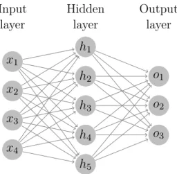
neural network (NN) is a family of computational learning systems inspired by biological
neural circuits in a human brain. NNs without cyclic connections between nodes, namely
feed-forward neural network (FNN), are used for building non-linear classifiers. Thus, NNs
learn more complex decision boundaries than LR models.
Recently, tremendous efforts have been devoted to improving the performance of neural networks with multiple layers of abstraction, which lead to many successful applications in a variety of areas for solving complex problems in artificial intelligence. The first successful examples of deep neural network (DNN) have been built by iteratively stacking multiple
More complex NNs that exploit spatial or temporal structures in data have been also very successful in learning representations of inputs from data as well as parametric classifiers (Krizhevsky et al., 2012;Sutskever et al.,2014). Massively parallel computing architectures such as graphics processing units (GPUs) and many large-scale datasets have proliferated
this research field even further over the last years.
Despite their effectiveness in learning complex functions such as classifiers, NNs have re-ceived less attention in MLC. A well-known NN-based MLC architecture (Zhang and Zhou,
2006),backpropagation for multi-label learning (BP-MLL), is problematic because it is
com-putationally demanding to make use of label dependency patterns on large-scale datasets. Modeling pairwise label dependencies in NNs explicitly makes it difficult for us to build more powerful neural architectures, which learn meaningful intermediate representations from data.
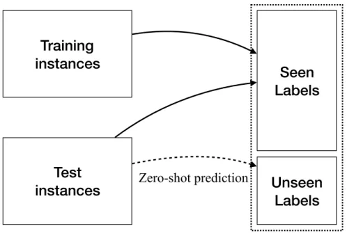
Exploiting additional information on label spaces. In a general workflow, MLC methods learn from only a set of training examples, where the association patterns of instances and labels are available. While training MLC models on the patterns, we expect that they are able to uncover underlying relationships between labels once training is done. The learned information during the training phase helps us make better predictions on unseen instances, where the label space on which MLC models are trained remains the same at prediction time. As an extreme case, one can assume we may receive unseen instances associated with unseen labels as well as seen labels. In other words, some labels in a set of candidate labels
to be predicted have no training instances, so that it is crucial to exploit label dependence if we want to make predictions over label spaces including unseen labels. Figure 1.2 shows the difference between traditional classification and zero-shot learning (ZSL). Traditional
classification tasks aim at learning mapping functions from training instances to the set of labels in the training set, and then test (unseen) instances are mapped the same set of labels observed during the training time (solid line). In contrast to the conventional setting of classification, we seek a function that maps test instances to a set of unseen labels (dotted line) for ZSL. The underlying assumption in ZSL is that the disjoint label sets, i.e., seen and unseen labels, share some information explicitly or implicitly.
When building MLC systems that have the capability to predict unseen labels, a major issue is the limited information problem of the relationships between seen and unseen labels, which we cannot access in a given training dataset. To bridge the gap between the problem of interest and the information available, one may consider external resources, e.g., knowledge bases, that human experts have organized. The central idea is that label relationships can be extracted if we can find mappings from labels to entities in external resources. This line of research has recently emerged in the machine learning community and is referred to as ZSL. In the literature, there have been several ZSL approaches that take advantage of the recent advancements in learning DNNs. Given side information that describes class labels with human curated annotations, we can exploit it to transfer information between seen and unseen labels (Lampert et al., 2009). This approach assumes that high-level semantic attributes for class labels are predefined by human experts, but it is also possible to utilize textual information on the web for building automatic ZSL systems (Frome et al., 2013).
The key property on which ZSL methods rely is the label dependence. Once learned shared information on seen labels, a ZSL classifier is able to transfer knowledge to predict unseen labels. As noted, it is also important for MLC methods to exploit the label dependence as
Training
instances
Seen
Labels
Test
instances
Unseen
Labels
Zero-shot prediction
Figure 1.2:Illustration of zero-shot learning.
in ZSL. This implies that the basic ideas for ZSL can be adopted to MLC methods, and it may bring us better predictive MLC systems in practice.
A problem may arise when taking label dependencies even between seen and unseen labels on MLC datasets with many labels into account due to the cost of preparing the information by human experts. Therefore, it is highly desirable to learn shared information between labels in an automatic way as in (Socher et al., 2013) for MLC.
1.1 Summary of Contributions
Given the aforementioned challenges, the goal of this thesis is to present neural network based extensions to existing approaches for the multi-label classification problems in the following:
• New insights on neural network architectures for multi-label classification are provided based on recent theoretical analyses in terms of consistency.
• Efficient neural network models on large-scale text datasets with many labels are pre-sented.
• We propose how to exploit the label dependence with neural networks.
• Towards predicting unseen labels, we present neural networks that make use of addi-tional information on label spaces.
1.2 Thesis Outline
The rest of the thesis is structured in the following way. After providing fundamentals of MLC and NNs in Chapter 2, we present our contributions in the subsequent chapters. Chapter 3 proposes a simple, yet effective NN architecture that minimizes the number of
incorrect pairwise rankings between relevant and irrelevant labels. Subsequently, in Chap-ter4we proposerecurrent neural networks (RNNs) as a replacement ofprobabilistic classifier chain (PCC) approaches that maximizes the probability of predicting label subsets correctly.
We, then, demonstrate the use of label structures represented as a graph for unseen label prediction in Chapter 5. In Chapter 6 we use label descriptions as a source of additional information for ZSL. Our goal is not only to obtain better zero-shot predictions, but also to improve generalization performance to seen labels. Lastly, we conclude our contributions and discuss future work for MLC in Chapter 7.
In the following, we provide an overview of the remaining chapters.
Background. MLC is the generalized problem of classifying instances into multiple classes, where more than one label may need to be assigned to each instance. We build a general framework for MLC in a theoretical point of view, followed by reviews of prior work that have been successfully applied in the literature. Generally, MLC methods are evaluated in terms of several aspects of their performance because different group of approaches often have different objectives to be optimized. Therefore, we discuss multiple evaluation measures commonly used in MLC.
Then, we cover fundamentals of NNs, on which all methods proposed in this thesis will be based.
Efficient neural networks for large-scale multi-label classification. A key objective of MLC is to capture label dependencies so as to make better predictions for unseen instances, and many successful MLC methods rely on computationally expensive operations to achieve the goal. In particular, it is difficult to apply this type of approach on problems which have a larger number of labels because the complexity grows in terms of the number of labels. Although there have been proposed NN architectures that capture label dependencies ex-plicitly on the output layer, we found that FNNs outperform more complex NNs on several text benchmark datasets in terms of ranking measures Nam et al.(2014). We show its the-oretical background and provide empirical analysis that suggests effective NN architectures formulti-label text classification (MLTC) in Chapter 3.
Estimating joint probabilities of label subsets using label sequences. In contrast to MLC methods that optimize the ranking objectives, where a ranked list of labels generated by MLC systems is compared to a true ranking of labels, another type of methods focus on building a classifier that produces a set of binary predictions. One of the most successful methods in this direction is PCC, which constructs a chain of independent classifiers per label and yields the final predictions. After the success of PCC, many MLC algorithms have been proposed to address its major limitations such as the computational complexity of searching over a label space that grows exponentially in labels.
However, another drawback of PCC is often disregarded: its performance decreases as the chain length gets longer. Using the fact that the average number of labels assigned to instances is much less than the total number of labels in general, we propose a RNN architecture for solving MLC problems as an alternative of PCC (Nam et al.,2017). Our ex-perimental results on three multi-label textual datasets demonstrate that RNNs are effective multi-label classifiers particularly when we have a large number of labels.
Learning from label hierarchies. Identifying relationship among labels from statistical pat-terns of them available in data is crucial to build MLC systems because the performance of predictive systems depends usually on the availability of training data and its quality. In both of the previous chapters (Chapter3 and 4), we mainly discuss the way to make use of the label patterns only and the effectiveness of NNs. One can also consider training MLC systems in which the data is scarce or even it is completely unavailable for certain labels. For example, given a database of scientific articles, new articles could be added to the database at a certain time interval, and we want to annotate them with MLC algorithms which is trained on the database previously. In this case, there is a chance that some of new articles may deal with something new which cannot be annotated by any of existing labels used at training time.
In Chapter 5, we propose an algorithm that has the capability to rank labels including ones that do not have training information (Nam et al., 2015). We take advantage of label relationships in a graph structure given as additional information, thereby achieving better label rankings if unseen labels are taken into account at test time.
Discovering latent structures from label descriptions. Label relationships as additional information are useful for a certain type of problem as discussed in Chapter 5. However, it is not always possible to obtain the label relationships as part of the training information. One can make use of another indirect information from which label relationships can be derived implicitly, and a label description in text is a good alternative for this purpose (Nam et al.,2016). Assuming that we are given textual descriptions for unseen labels, it might be possible to predict onunseen documents with respect to evenunseenlabels if we can leverage
the fact that similar labels often have similar word usage patterns in the descriptions. For example, assuming an organization as a label, we can easily find a textual description of the organization on the web, e.g., Wikipedia (Roth, 2017).
2 Background
In this chapter, we will provide the definition of multi-label classification (MLC) as an area
of machine learning. Let us start with binary classification to formulate the learning problem in a statistical way and then extend it to multi-label classification.
2.1 Binary Classification and Risk Minimization
Binary classification is the task of classifying instances into two groups. In other words, we seek a function f that returns predicted outputs yˆ ∈ {0,1} of inputs xxx, i.e., f : XXX → YYY oryˆ= f(xxx). Given a loss function `: (y,yˆ)→ R which measures the discrepancy between
true targets y and predictions y, let us define the expected loss of a functionˆ f over data samples from an underlying probability distribution P(XXX, YYY) as expected ortrue risk R:
R(f) =EXXXYYY [`(YYY , f(XXX))]. (2.1)
The quality of a mapping function can be determined by comparing the risk of the function to that of other functions, for example, a functionf is better thang ifR(f) <R(g)(Vapnik,
1999). One can find the best function which achieves the smallest risk over all possible functions. Formally, let us defineminimum risk or Bayes risk as follows
R∗ = inf
f∈FallR(f) (2.2)
whereFall denotes a set of all possible measurable functions mapping inputsXXX to outputs
Y Y
Y. A function that satisfies R∗ =
R(f) is called as a Bayes classifier. Assuming that we
have perfect knowledge on P(XXX, YYY), the Bayes classifier for binary classification problems
can be defined as follows
f∗(xxx) =
¨
1 if P(YYY = 1|XXX = xxx)≥ 1 2
0 otherwise (2.3)
where P(YYY = 1|XXX = xxx) is the conditional probability that an instance xxx is classified as positive. Please note that Eq. (2.3) can be generalized to multi-class classification. As the underlying distribution P(XXX, YYY) is unknown in general, it is impossible to calculate the
Bayes classifier. Given a function class such that F ⊆ Fall and a set of N training data
D = {(xxx1, y1),(xxx2, y2),· · · ,(xxxN, yN)} sampled from the underlying distribution, one can
select a function fN ∈ F and calculate its empirical risk given by
Remp(fN) = 1 N N X n=1 `(yn, fN(xxxn)). (2.4)
The objective of selectingfN ∈ F given the data is to achieveminimum empirical risk while
keeping the difference between the empirical risk and true risk, e.g., |R(fN)− Remp(fN)|,
small. Please note that the function space F may or may not include the target function,
i.e., the Bayes classifier. If the loss is viewed as a random variable that maps predicted outputs fN(xxx) to real numbers, i.e., error rates with respect to true targets, the empirical
risk converges to the true risk as the number of samples N goes to infinity by the law of large numbers:
Remp(fN)→ R(fN) when N → ∞. (2.5)
The next question is a way to measure how close the empirical risk of any (fixed) clas-sifier f to its true risk. Note that for its simplicity we assume that f does not de-pend on data samples. Hoeffding’s inequality provides an upper bound of the probability that the difference between the sample average of random variables and its true expec-tation is smaller than some arbitrary number. Without loss of generality, suppose that Z1 = `(y1, f(xxx1)),· · · , ZN = `(yN, f(xxxN)) are i.i.d. random variables bounded in the
range [0,1], which allows us to rewrite the difference between two risks as follows
Remp(f)− R(f) = 1 N N X n=1 Zn−E[ZZZ]. (2.6)
Then, for all ≥0, we have
P 1 N N X n=1 Zn−E[ZZZ] ≥ ≤2 exp(−2N 2). (2.7) If we denote the r.h.s. of Eq. (2.7) by δ, i.e., δ = 2 exp(−2N 2), it tells us that with probability at least 1− δ the difference between the empirical risk 1
N
PN
n=1`(yn, f(xxxn)) and the true risk EXXXYYY [`(YYY , f(XXX))] is within a certain constant . We can interpret δ
as a significance level or 100 × (1 − δ)% as confidence where its confidence interval is [E[Z]−,E[Z] +]. To be more precise, we can rewrite Eq. (2.7) as follows
1 N N X n=1 Zn−E[ZZZ] ≤ (2.8)
which holds with probability at least1−δ. We can interpret asaccuracy of the empirical
risk with respect to the true risk. Furthermore, we can derive an interesting relationship between the number of samplesN and the two parameters of Hoeffding’s inequality δ, :
N ≥ 1
22 log
2
δ. (2.9)
As expected, Eq. (2.9) shows that to increase the accuracy and significance δ, we need more training samples. Rearranging N and in Eq. (2.9) and plugging it into Eq. (2.8), we have the following relationship between the true risk and empirical risk of any classifier f:
R(f) ≤ Remp(f) + v t 1 2N log 2 δ. (2.10)
Note that this bound holds only if we use an arbitrary but fixed classifier f that does not change depending on training samples.
Estimation error Approximation error F fN fF f∗
Figure 2.1:Illustration of the regret decomposition.
Consistency We now have an upper bound of the empirical risk. Given a set of train-ing examples D = {(xxxn, yyyn)}
N
n=1 following a fixed (but unknown) probability distribution P(XXX, YYY), let A be a learning algorithm that chooses a function (i.e., classifier) fN from a
set of measurable functions F.1 If the risk of f
N, i.e., R(fN), approaches the Bayes risk
R∗ with high probability as the number of training examples gets large, A is called Bayes consistent with respect to the probability distribution P(XXX, YYY) and a loss function ` used for calculating the risk:
P (R(fN)− R(f∗)> )→0 as N → ∞,∀ >0. (2.11)
Note that we can interpret R(fN) as a random variable that measures fN estimated by A
on given a finite number of sample dataD. The difference between the risk of fN and the
Bayes classifierf∗ is often referred to as excess risk or regret
regret`,P(fN) =R(fN)− R(f∗) (2.12)
which can be decomposed into two terms:
R(fN)− R(f∗) = R(fN)− inf f∈FR(f) + inf f∈FR(f)− R(f ∗ ) . (2.13) The first term is called the estimation error and the second one is the approximation error.
The estimation error measures how much the functionfN is close to the best possible function
in the function spaceF while the approximation error measures the discrepancy between the
optimal error inF and the Bayes risk. The error decomposition is illustrated in Figure 2.1.
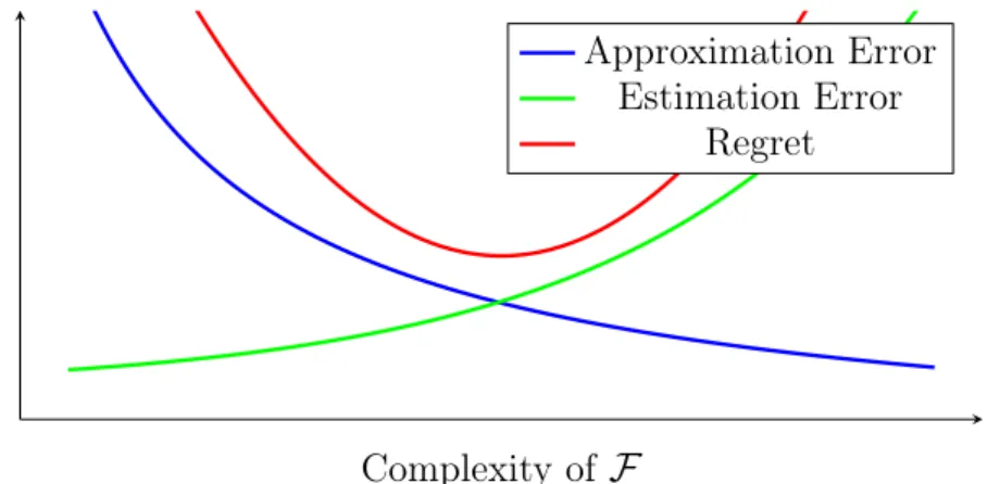
When a larger function space is considered for A, the approximation error decreases while the estimation error may increase. On the other hand, a smaller function space F allows to decrease the estimation error, but this may result in higher approximation error depending on F. There is a tradeoff between both errors, which is also known as the bias-variance
trade-off. Usually it is hard to estimate the approximation error since it requires knowledge about the target such asP(YYY|XXX). In machine learning we make assumptions on the optimal
functionsfF so as to minimize the estimation error. 2.2 Multi-label Classification
Multi-label classification (MLC) is the task of learning a function f that maps inputs to subsets of a label set L= {1,2,· · · , L}. Consider a set of N samples D = {(xxxn, yyyn)}Nn=1, 1 Informally, a function is measurable if its outcome is not infinitely sensitive to small changes in input.
Complexity of F
Approximation Error Estimation Error
Regret
Figure 2.2:The estimation error and approximation error vary according to the complexity of the function spaceF.
Table 2.1:An example of multi-label instances
features labels x1 x2 x3 x4 x5 x6 x7 x8 y1 y2 y3 y4 Training dataset D −1.5 0.0 1.8 0.4 0.7 1.0 −1.4 0.4 1 0 1 0 1.9 0.9 −0.1 0.8 0.8 1.1 −0.9 0.5 0 0 1 1 −0.8 0.1 0.1 −2.3 0.7 −1.4 0.8 −1.3 1 1 0 1 0.9 0.0 1.1 0.2 −0.1 −0.4 −1.2 −0.1 0 0 1 0 −1.3 −1.3 0.2 1.3 −1.4 −1.7 −1.1 −0.3 0 1 0 0 −0.9 −1.4 0.8 −0.2 0.1 1.3 0.0 −0.3 1 1 1 0 Test dataset Du −0.5 −1.4 0.9 −0.9 −0.6 −0.8 −0.2 −2.7 ? ? ? ? 0.3 0.8 −0.3 −0.5 −0.6 0.5 0.2 −0.9 ? ? ? ? −0.8 −1.4 1.0 −1.1 0.6 −2.0 0.9 0.8 ? ? ? ?
each of which consists of an input xxx and its target yyy. The pairs (xxxn, yyyn) are assumed to be i.i.d. random variables following an unknown distributionP(XXX, YYY).We letTn = |yyyn|denote
the size of the label set associated to xxxn and C = N1
PN
n=1Tn the cardinality of D, which is usually much smaller thanL. Often, it is convenient to view the target yyy not as a subset of L but as a binary vector of size L, i.e., yyy ∈ {0,1}L. Let us denote a set of N
ts unseen instances byDu = {(xxxu ¯ n, yyyun¯)} Nts ¯
n=1 following the same unknown distributionP(XXX, YYY). Once the functionf is learned from D, at test time, we usef to make predictionsyyyˆu for givenxxxu.
The goal of learningf is to minimize the expected loss of instances following the underlying distributionP:
min
f E(xxx,yyy)∼P [`(yyy, f(xxx))]. (2.14)
Table 2.1 shows exemplary training and test instances. We have 6 training instances repre-sented in 8 features and each instance is associated with 4 dimensional binary vector. The label vectorsyyycontain multiple elements of 1. Given the training instances, we want to find the most probable label vectorsyyyˆ ∈ {0,1}4 for the given input features of 3 test instances.
In a probabilistic point of view, MLC can be understood as a task of estimating the underlying distribution P(XXX, YYY) from the training dataset D. Since in MLC instances xxx
are available, it would be easier to estimate the conditional distribution of labelsYYY given an instancexxx, i.e., P(YYY|XXX =xxx), than the complete joint distributionP(XXX, YYY).
Assigning a subset of labels to an instance is equivalent to predicting the most probable label subset out of a label powerset SL = {∅,{1},{2},· · · ,{1,2,· · · , L}}. To achieve the
goal, ideally, we need to calculate the joint probability of labels for a given instance:
P (yyy|xxx) =P (y1, y2,· · · , yL|xxx) (2.15)
where y ∈ {0,1}. Then, a label subset which yields the maximum value is chosen as an output. As the computational complexity of finding the maximum value of the joint probability of labels grows exponentially in the number of labels, i.e., |SL| = 2L, one can
come up with a simpler solution by estimating the marginal probability of each label based on the strong assumption that labels are independent conditional on xxx. That is, the joint probability of labels can be factorized as
P(yyy|xxx) =
L
Y
i=1
P(yi= 1|xxx) (2.16)
where yi = 1 denotes label i is associated with a given instance xxx. Although such an
assumption allows us to reduce the complexity fromO(2L) to
O(L), it yields a suboptimal
solution to estimating the joint probability of labels.
Let us explain why the joint probability is needed for choosing the most relevant label subset with a concrete example. Let YYY = {Y1, Y2} be a label space and Yi be binary
random variables. Table2.2 shows an example of the joint probability P(YYY =yyy|xxx) and the
marginal probabilitiesP(Y1 = y1|xxx) and P(Y2 =y2|xxx).
Table 2.2:An example of the joint probability of labelsYYY ={Y1, Y2}given an instancexxx.
P(YYY|xxx) 0 y1 1 P(Y2|xxx) y2 01 0.0 0.40.3 0.3 0.40.6 P(Y1|xxx) 0.3 0.7 1
Let us denote by yyy∗joint = {yjoint∗ ,1, y∗joint,2} the mode of the joint probability of labels and yyy∗marginal= {ymarginal∗ ,1, ymarginal∗ ,2}the set of the mode of the marginal probabilities. In this example, the mode of the joint probability of labels is yyy∗joint = {1,0} where we have the maximum joint probabilityP(YYY = yyy∗joint|xxx) = 0.4. By summingP(Y1, Y2|xxx)for all possible values ofYi, we obtain the marginal probabilities P(Y1|xxx) and P(Y2|xxx). As can be seen in Table2.2, we have yyy∗marginal= {1,1}and it does not match the mode of the joint probability
of labels:
yyy∗joint6= yyy∗marginal
Although there are few exceptions where the relationship betweenyyy∗joint and yyy∗marginal does not hold (which shall be discussed shortly), in general, one needs to take the joint probability of labels into account when building a MLC system (Dembczyński et al., 2010). Hence, the
Table 2.3:Example-based evaluation
Target labels Predicted labels Subset accuracy
y1 y2 y3 y4 yˆ1 yˆ2 yˆ3 yˆ4 `(yyy,ˆyyy) 1 0 1 0 0 1 1 0 0 0 0 1 1 1 0 1 0 0 1 1 0 1 1 1 0 1 1 0 0 1 0 0 0 1 0 1 0 1 0 0 1 0 0 0 0 1 1 1 0 1 1 0 1 0 0.33
key issue of MLC is how to design classification systems estimating the joint probability of labels under some constraints related to problem domains, the scale of the problem, the availability of resources, etc.
An obvious way of evaluating MLC systems is to count how many times the systems predict a subset of labels correctly with respect to the target label subset. Depending on the goals of MLC systems, however, we are interested in different aspects of system outputs to get a better understanding of problems and results of our design choices. In the next section, we will discuss several evaluation measures that are widely used in the literature.
2.2.1 Evaluation Measures for Multi-label Classification
MLC algorithms can be evaluated with multiple measures which capture different aspects of the problem. We evaluate all methods in terms of both example-based and label-based measures.
Example-based measures are defined by comparing, for each example, the target vector yyy= {y1, y2,· · · , yL} to the prediction vector ˆyyy= {yˆ1,yˆ2,· · · ,yˆL} for a given example, and
averaging the results over all examples.
Subset accuracy (ACC) checks whether a predicted label vectoryyymatches its targetexactly
or not as follows
ACC(yyy,yyyˆ) =I[yyy = ˆyyy] (2.17)
where I[·] returns 1 if its argument is true otherwise 0. It is very strict to incorrectly
predicted labels in that it does not allow any deviation in the predicted label set.
Hamming accuracy (HA) computes how many labels are correctly predicted in ˆyyy: HA(yyy,ˆyyy) = 1 L L X j=1 I[yj = ˆyj]. (2.18)
Both, ACC and HA can be used for datasets with moderate label set sizes L. If the label cardinality of a dataset is higher, entirely correct predictions become increasingly unlikely,
and therefore ACC often approaches 0. In this case, the example-based F1-measure (ebF1) can be considered as a good compromise:
ebF1(yyy,yyyˆ) =
2PL j=1yjyˆj PL j=1yj + PL j=1yˆj . (2.19)
A concrete example of example-based evaluation using ACC is shown in Table 2.3. MLC also can be viewed as a ranking problem. In order to evaluate the quality of a ranked list, we consider several ranking measures (Schapire and Singer, 2000). Given an instance x
x
x and associated label information yyy, consider a multi-label learner fθ(xxx) that is able to
produce scores for each label. These scores, then, can be sorted in descending order. Let r(y)be the rank of a labelyin the sorted list of labels. The most intuitive objective for MLC is to minimize the number of misorderings between a pair of relevant label and irrelevant label. This is called the rank loss (RL):
RL(yyy,yyyˆ) =w(yyy) X
yi<yj
I(ˆyi > yˆj) +
1
2I(ˆyi = ˆyj) (2.20)
wherew(yyy) is a normalization factor, I(·) is the indicator function.
One error (1-err) evaluates whether the top most ranked label with the highest score is a
positive label or not:
1-err(yyy,ˆyyy) =I r−1(1) ∈/ yyy (2.21)
wherer−1(1) indicates the index of a label positioning on the first place in the sorted list of predicted labelsy.ˆ
Coverage (Cov) measures on average how far one needs to go down the ranked list of labels
to achieve recall of 100%:
Cov(yyy,ˆyyy) = max
yi∈yyy r(yi)−1 (2.22) Average precision (AvgP) measures the average fraction of labels preceding relevant labels
in the ranked list of labels:
AvgP (yyy,yyyˆ) = 1
|yyy| X yi∈yyy |{yj ∈yyy|r(yj)≤r(yi)}| r(yi) (2.23) Label-based measures are based on treating each labelyjas a separate two-class prediction
problem, and computing the number of true positives (tpj), false positives (fpj) and false negatives (fnj) for this label as follows
tpj = N X n=1 I[ynj = 1∧yˆnj = 1] f pj = N X n=1 I[ynj = 1∧yˆnj = 0] f nj = N X n=1 I[ynj = 0∧yˆnj = 1] (2.24)
Table 2.4:Label-based evaluation
yyy Target labels Predicted labels Macro-averagedF1
tp fp fn y1 1 0 1 0 0 1 0 1 1 0 1 1 2 2 1 0.68 y2 0 0 1 0 1 1 1 0 1 0 0 1 2 1 1 y3 1 1 0 1 0 1 1 1 0 1 0 0 3 0 0 y4 0 1 1 0 0 0 0 0 1 0 0 1 1 1 1
We consider two label-based measures, micro-averaged F1 (miF1) miF1 YYY ,YYYˆ = PL j=12tpj PL j=12tpj+fpj+fnj , and macro-averaged F1 (maF1)
maF1 YYY ,YYYˆ = 1 L L X j=1 2tpj 2tpj+fpj+fnj
whereYYY is the N×L matrix where ynj correspond to the true label j of the n-th instance
x
xxn, and YYYˆ is the matrix of predictions yˆnj.
While miF1 favors a system yielding good predictions on majority labels, higher maF1 scores are usually attributed to superior performance on minority labels. Table2.4shows how to calculate maF1 on the same pairs of the target and predicted label vectors as Table2.3.
2.2.2 Risk Minimization for Multi-label Classification
We have discussed several evaluation measures commonly used in the context of MLC in the previous section. Although we want to build MLC systems that perform well across multiple measures, it is a very challenging objective to achieve the goal in general. In other words, it is likely that a system yielding good performance in terms of a certain evaluation measure may perform worse in another measure. In this section we will discuss the relationship between different models, each of which is trained to minimize different loss functions.
The goal of MLC is to find an optimal function f∗ that minimizes the expected loss on an unknown sample drawn fromP(XXX, YYY):
f∗ = arg min f EXXXYYY [`(YYY , f(XXX))] = arg min f E X X X EYYY|XXX [`(YYY , f(XXX))] . (2.25)
While the expected risk minimization over P(XXX, YYY) is intractable, for a given observation
x xx it can be simplified to f∗(xxx) = arg min f EYYY|XXX [`(YYY , f(xxx))] = arg min f Z `(YYY , f(xxx))dP(YYY|XXX = xxx). (2.26)
Let us consider two evaluation measures: HA and ACC. Whereas HA calculates the pre-diction accuracy per label independently, ACC favors only prepre-diction results yyyˆ that match
their targets yyy exactly. Since we want to minimize risk, let `h(yyy,yyyˆ) and `s(yyy,ˆyyy) be the
Hamming loss and subset 0/1 loss, respectively, as follows `h(yyy,ˆyyy) = 1 L L X j=1 I[yj 6= ˆyj] (2.27)
`s(yyy,ˆyyy) =I[yyy 6= ˆyyy] (2.28)
where bothyyyandˆyyyareL-dimensional binary vectors. Using the loss functions, let us denote the optimal functions in terms of the Hamming loss and subset 0/1 loss given by
fh∗(xxx) = arg min f EYYY|XXX [`h(YYY , f(xxx))] (2.29) fs∗(xxx) = arg min f EY YY|XXX [`s(YYY , f(xxx))] (2.30) where f∗ h(xxx) and f ∗
h(xxx) denote Bayes classifiers in terms of the Hamming loss and subset
0/1 loss, respectively.
Let us begin with calculating the Bayes classifier with respect to the subset 0/1 loss. Since both targets yyy and predictions yyy are defined as binary (discrete) vectors, we can calculate the expected loss of predictionsyyyˆ that a function f returns for given xxx as follows
EYYY|XXX[`s(YYY ,yyyˆ)] =
X
y yy
`s(yyy,yyyˆ)P(YYY = yyy|XXX =xxx)
= X
y yy
(1−I[yyy = ˆyyy])P(YYY =yyy|XXX =xxx)
= X y yy P(YYY =yyy|XXX =xxx)−X y y y
I[yyy= ˆyyy]P(YYY =yyy|XXX = xxx).
(2.31)
In fact, the second term on the r.h.s. of Eq. (2.31) is calculated by a summation over 2L
label configurations. We also know that the function output ˆyyy is fixed given a function, which enables us to factorize the second term into two parts. One is the joint probability of yyy which is equal to yyy. The other is the sum of the joint probabilities of the rest of labelˆ
combinations, which is equal to zero. More precisely, we can rewrite the second term on the r.h.s. of Eq. (2.31) as follows
X
y yy
I[yyy = ˆyyy]P(YYY = ˆyyy|XXX = xxx) =P(YYY = ˆyyy|XXX =xxx)
+X
y y y6=ˆyyy
I[yyy= ˆyyy]P(YYY = yyy|XXX = xxx)
| {z }
=0because ofI[yyy=ˆyyy]=0,∀yyyin the sum
(2.32)
= P(YYY = ˆyyy|XXX =xxx). (2.33) Plugging Eq. (2.33) into Eq. (2.31), we have
Thus, the expected risk minimization in terms of the subset 0/1 loss is equivalent to finding a mode of the joint probability of labelsYYY given instancesxxx and the Bayes classifier is given by
fs∗(xxx) = arg max f
P(YYY = ˆyyy|XXX = xxx). (2.35) Similarly, we can also calculate the Bayes classifier in terms of the Hamming loss. Let us
rewrite the expected risk in terms of the Hamming loss using definition of the loss function as follows EYYY|XXX[`h(YYY ,ˆyyy)] = X y y y
`h(yyy,ˆyyy)P(YYY = yyy|XXX = xxx)
= 1 L X y1,y2,···,yL yj∈{0,1} `1 h(y1,yˆ1) +· · ·+` L h(yL,yˆL) P(YYY = yyy|XXX =xxx) (2.36) where `jh yj,ˆjj = Iyj 6= ˆjj
. As the hamming loss treats each label independently that allows us to assume labelsyj are conditionally independent, we can factorize the summation
on the r.h.s. of Eq. (2.36) as follows X y1,y2,···,yL yj∈{0,1} `1h(y1,yˆ1) +· · ·+`Lh (yL,yˆL) P(YYY =yyy|XXX = xxx) = X y1∈{0,1} (1−I[y1 = ˆy1])P(Y1 =y1|XXX =xxx) + X y2∈{0,1} (1−I[y2 = ˆy2])P(Y2= y2|XXX = xxx) +· · ·+ X yL∈{0,1} (1−I[yL= ˆyL])P(YL =yL|XXX = xxx) =L−X j=1 P(Yj = ˆyj|XXX = xxx). (2.37)
In turn, substitution of Eq. (2.36) with Eq. (2.37) gives
EYYY|XXX [`h(YYY ,yyyˆ)] = 1− 1 L L X j=1 P(Yj = ˆyj|XXX = xxx). (2.38)
The expected risk minimization in terms of the hamming loss is equivalent to finding L marginal modes ofYj given instances xxx independently, and the Bayes classifier is given by
fh∗(xxx) ={arg max
f1
P(Y1 = ˆy1|XXX =xxx),· · · ,arg max
fL
P(YL= ˆyL|XXX =xxx)}. (2.39)
In contrast to that the Bayes classifier for the subset 0/1 loss fs∗(xxx) requires the joint
probability distribution of labels, we can obtain the Bayes classifier for the hamming loss
Table 2.5:TheBayes classifiers for the Hamming loss and subset 0/1 loss are identical if (a) labels are conditionally independent or (b) the joint mode of labels are greater than or equal to 0.5.
(a) P(YYY|xxx) 0 y1 1 P(Y2|xxx) y2 01 0.12 0.180.28 0.42 0.30.7 P(Y1|xxx) 0.4 0.6 1 (b) P(YYY|xxx) 0 y1 1 P(Y2|xxx) y2 01 0.6 0.10.1 0.2 0.70.3 P(Y1|xxx) 0.7 0.3 1
As shown already in Table 2.2, the mode of the joint distribution of labels may differ from a set of marginal modes of individual labels except for two conditions where theBayes
classifiers for the subset 0/1 loss and hamming loss coincide. Assuming that all labels are
conditionally independent given instances such that P(Y1, Y2,· · · , YL|xxx) =
QL
j=1P(Yj|xxx), fh∗(xxx) and fh∗(xxx) are same. When a probability assigned to a single label configuration is
greater or equal to 0.5, i.e., P(YYY = f∗
s(xxx)|XXX = xxx) ≥ 0.5, fh∗(xxx) and f
∗
h(xxx) also return the
same function output. Table 2.5 shows two examples of such a probability distribution of labels.
We have discussed that the hamming loss and subset 0/1 loss lead us to different optimal functions. One can be obtained by ignoring label dependence completely, but the other seeks a label configuration that yields the highest probability over the entire label space. Due to the difference, it is unable to find a universal classifier that performs well across all measures. For example, Dembczyński et al. (2012b) have analyzed that the regret in terms of the subset 0/1 loss for the hamming loss is quite high and vice versa.
To be more specific, let us consider the regret of theBayes classifier for the hamming loss
in terms of the subset 0/1 loss. In other words, we compare the performance of f∗
h and f
∗
s
using the subset 0/1 loss. The upper bound of the regret is given by
EYYY|XXX[`s(YYY , fh∗(xxx))]−EYYY|XXX [`s(YYY , fs∗(xxx))]< 0.5. (2.40)
Please note that the risk of fh∗ and fs∗ in terms of the subset 0/1 loss are identical when
P(YYY =f∗
s(xxx)|XXX = xxx)≥0.5, so that the risk of fs∗ is greater than 0.5 if fh∗ differs from f
∗
s.
It is also worth noting that the risk of any classifier f is bounded by[0,1].
The regret offs∗ in terms of the hamming loss has the following upper bound forL >3: EYYY|XXX[`h(YYY , fs∗(xxx))]−EYYY|XXX[`h(YYY , fh∗(xxx))] <
L−2
L+ 2 (2.41)
For more details, please refer to (Dembczyński et al., 2012b).
In this section, we have shown that an optimal function for a certain evaluation measure may perform worse in terms of another measure. Hence, it is crucial to determine which evaluation measure will be optimized and to make sure the objective of a MLC system is consistent with respect to the measure of interest.
2.2.3 Multi-label Learning Algorithms
In this section, we discuss various existing approaches for MLC. The most straightforward way to tackle MLC is binary relevance (BR); it constructs L binary classifiers, which are
trained on the L labels independently. Thus, the prediction of the label set is composed of independent predictions for individual labels. Its predictive performance highly depends on a base learner. Support vector machines (SVMs), logistic regression (LR) and neural networks (NNs) are most commonly used in the literature for BR. The major drawback of
BR is that the label dependence is ignored, so that we cannot make use of the interesting characteristics in MLC problems, namely that the presence of a specific label may suppress or exhibit the likelihood of other labels.
Learning from pairwise label dependencies. Instead of trainingL independent classifiers in which label correlations are ignored, several approaches exploit the label dependence di-rectly in a single learning framework. A straightforward extension is to consider pairwise relationships between two labels. Elisseeff and Weston (2001) present a large-margin clas-sifier, RankSVM, that minimizes a ranking loss by penalizing incorrectly ordered pairs of labels. This setting can be used for MLC by assuming that the ranking algorithm has to rank each relevant label before each irrelevant label. In order to make a prediction, the ranking has to becalibrated (Fürnkranz et al., 2008), i.e., a threshold has to be found that splits the
ranking into relevant and irrelevant labels. Similarly, Zhang and Zhou(2006) introduced a framework that learns pairwise ranking errors in NNs,backpropagation for multi-label learn-ing (BP-MLL). Pairwise label dependencies are also used in graphical models for maximizing
subset accuracy (Ghamrawi and McCallum, 2005).
The methods based on pairwise comparisons have several limitations although they achieve competitive performance on the standard MLC benchmark datasets. Obviously, the total number of pairwise label dependencies affects the computational complexity, which grows quadratically in L. Thus, pairwise comparison based approaches do not scale on large data sets, specifically in the number of labels. Another limitation is the inability of learning higher-order dependencies which large-scale real-world datasets may contain more frequently than small benchmark datasets.
Subset accuracy maximization. To capture higher-order relationships among labels, there has been a family of approaches that attempt to classify a set of labels correctly instead of individual labels independently as in BR. The simplest approach in this direction, often referred to as subset accuracy maximization, is label powerset (LP). It reduces multi-label
classification into multi-class classification. In other words, LP assigns a unique class index to each subset of labels. While LP is appealing because most methods well studied in multi-class classification can be used, training LP models becomes intractable for large-scale problems with an increasing number of labels. Even if the number of labels L is small enough, the problem is still prone to suffer from data scarcity because each label subset in LP will in general only have a few training instances. An effective solution to these problems is to build an ensemble of LP models learning from randomly constructed small label subset spaces (Tsoumakas et al., 2011).
An alternative approach is to learn the joint probability of labels, which is again pro-hibitively expensive due to 2L label configurations. To address this problem, Dembczyński
et al. (2010) have proposed probabilistic classifier chain (PCC) which decomposes the joint
probability into L conditional probabilities: P(y1, y2,· · · , yL|xxx) =
L
Y
i=1
P(yi|yyy<i, xxx) (2.42)
where yyy<i = {y1,· · · , yi−1} denotes a set of labels that precede a label yi in computing
conditional probabilities, and yyy<i = ∅ if i = 1. For training PCCs, L functions need
to be learned independently to construct a probability tree with 2L leaf nodes. In other
words, PCCs construct a perfect binary tree of height L in which every node except the root node corresponds to a binary classifier. Therefore, obtaining the exact solution of such a probabilistic tree requires to find an optimal path from the root to a leaf node. A naïve approach for doing so requires2Lpath evaluations in the inference step, and is therefore also
intractable. However, several approaches have been proposed to reduce the computational complexity (Dembczyński et al., 2012; Kumar et al., 2013; Mena et al., 2015; Read et al.,
2014).
Apart from the computational issue, PCCs have also a few fundamental problems. One of them is a cascadation of errors as the length of a chain gets longer (Senge et al., 2014). During training, the classifiers fi in the chain are trained to reduce the errors E(yi,yˆi) by
enriching the input vectorsxxx with the corresponding previous true targetsyyy<i as additional features. In contrast, at test time, fi generates samples yˆi or estimates P(ˆyi|xxx,ˆyyy<i) where
ˆ
yyy<i are obtained from the preceding classifiers f1,· · · , fi−1.
Another key limitation of PCCs is that the classifiersfi are trained independently
accord-ing to a fixed label order, so that each classifier is only able to make predictions with respect to a single label in a chain of labels. Regardless of the order of labels, the product of condi-tional probabilities in Equation (2.15) represents the joint probability of labels by the chain rule, but in practice the label order in a chain has an impact on estimating the conditional probabilities. This issue was addressed in the past by ensemble averaging (Dembczyński et al., 2010; Read et al., 2011), ensemble pruning (Li and Zhou, 2013) or by a previous analysis of the label dependencies, e.g., by Bayes nets (Sucar et al., 2014), and selecting the ordering accordingly. Similar methods learning a global order over the labels have been pro-posed byKumar et al.(2013), who use kernel target alignment to order the chain according to the difficulty of the single-label problems, and by Liu and Tsang (2015), who formulate the problem of finding the globally optimal label order as a dynamic programming problem. Subset accuracy maximization has been also addressed by graphical models which extend
conditional random field (CRF) to MLC. Similar to CRFs, Ghamrawi and McCallum(2005)
proposecollective multi-label classifier (CML) andcollective multi-label with feature classifier
(CMLF) that define feature functions over pairs of label and input, and over pairwise label sets. The joint probability of labels given instances is then computed by the sum of all feature functions, followed by normalization. CML and CMLF have also the increasing complexity with respect to the possible number of label pairs. Li et al. (2016) introduce
conditional Bernoulli mixtures (CBMs), which are an extension of Bernoulli mixtures used
for multivariate density estimation in order to learn the joint distribution of labels in MLC. CBM learns a mixture of conditional binary label distributions, each of which represents the probability of a label given an instance. In contrast to CML and CMLF, CBM’s complexity grows linearly inL because it does not rely on label pairs to estimate the joint probability.